
Kernel Minimum Noise Fraction Transformation-Based Background Separation Model for Hyperspectral Anomaly Detection
 , , and
Abstract
:1. Introduction
- (1)
- To employ an effective feature extraction method before estimating anomalies and background, this article assesses the detection performance of KMNF and other feature extraction methods (including linear discriminant analysis (LDA), PCA, minimum noise fraction (MNF), optimized MNF (OMNF), factor analysis (FA), KPCA, optimized KMNF (OKMNF), local preserving projections (LPP), and locally linear embedding (LLE)) in AD for HSIs. The experimental results show the effectiveness and robustness of KMNF transformation in feature extraction for AD, which provides a reference for the application of feature extraction in AD.
- (2)
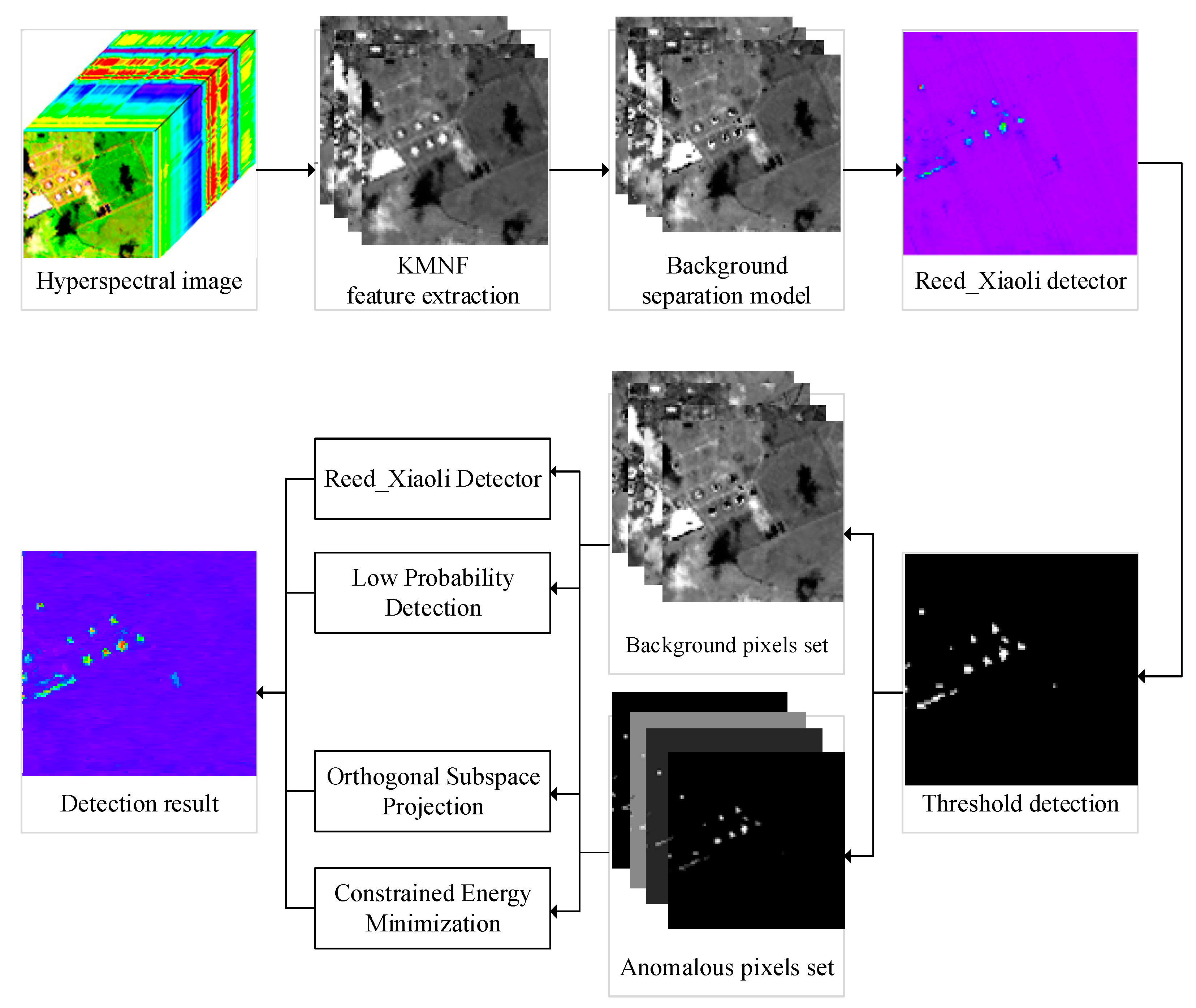
- Considering the high-order correlation between spectral bands in HSIs and the role of anomaly and background estimation in AD, a KMNF-BSM aiming at separating anomalies and background efficiently is proposed in this article. It can obtain accurate background and anomalous pixel sets, and it has significant anti-noise ability and adaptability to HSIs with different spatial and spectral resolutions, which offers a new solution for high-precision AD.
- (3)
- The proposed method achieves autonomous hyperspectral AD without pre-processing or post-processing procedures. It can accurately reconstruct the background and separate anomalies automatically, which solves the problem of low detection accuracy when the prior knowledge is insufficient for the supervised detection methods.
2. Proposed Methods
2.1. KMNF Transformation for Feature Extraction
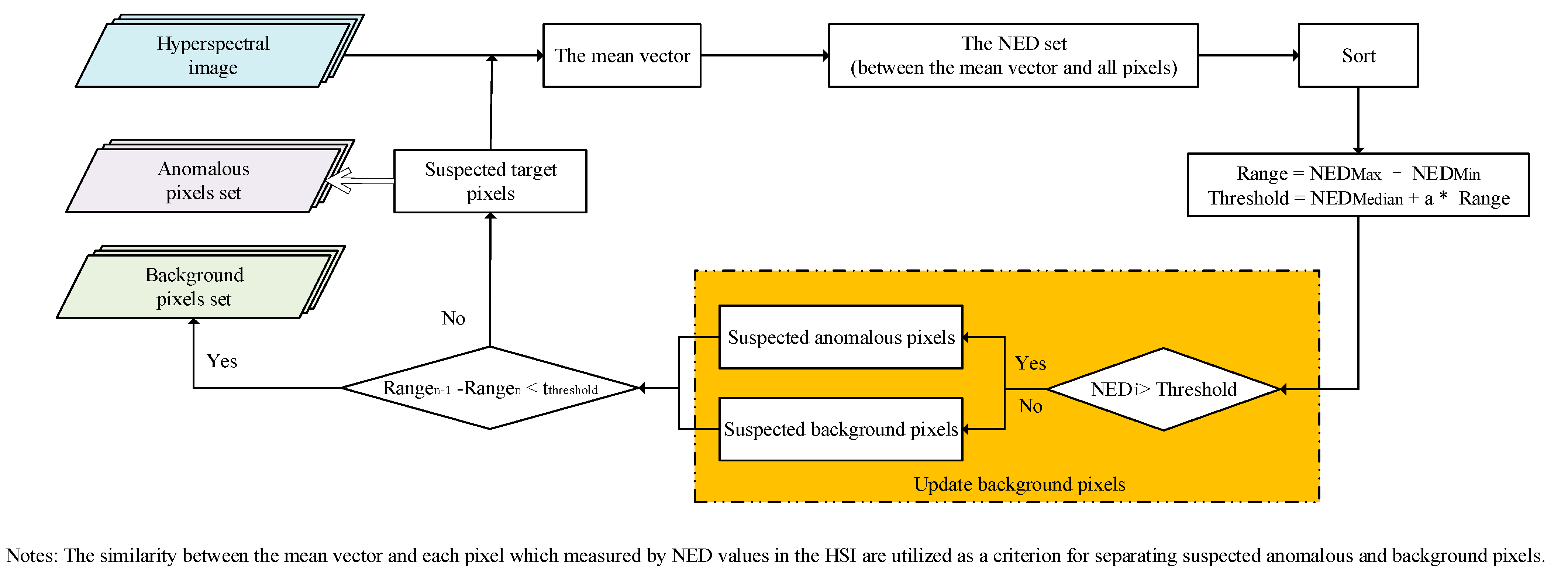
2.2. Background Separation Model (BSM)
2.3. KMNF-BSM-Based Anomaly Detectors
2.3.1. KMNF-BSM-RXD Algorithm
2.3.2. KMNF-BSM-LPD Algorithm
2.3.3. KMNF-BSM-OSPAD Algorithm
2.3.4. KMNF-BSM-CEMAD Algorithm
3. Results
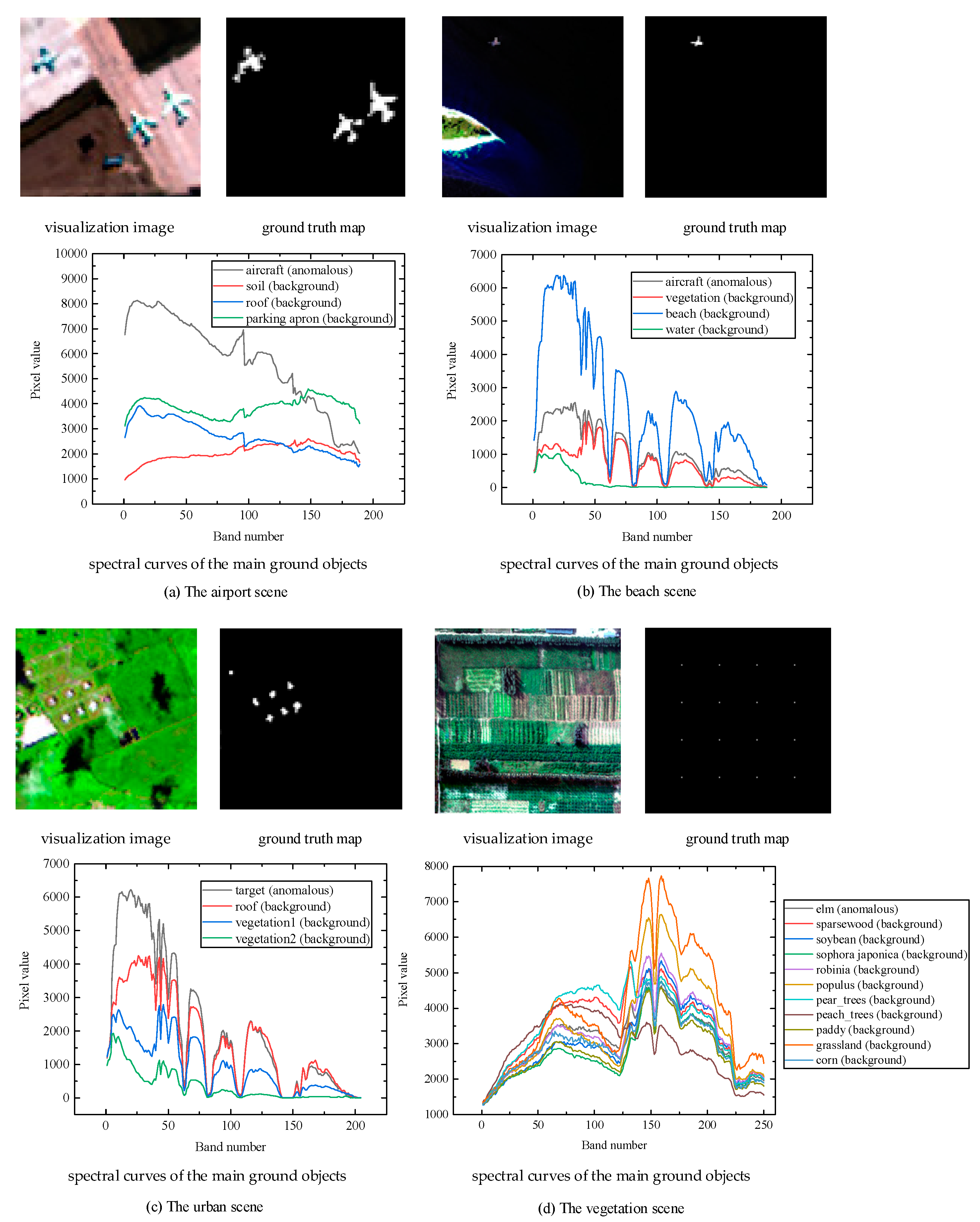
3.1. Input Data
3.1.1. San Diego Dataset
3.1.2. Airport–Beach–Urban Dataset
3.1.3. Xiong’an Dataset
3.2. Experimental Settings
3.2.1. Parameter Settings
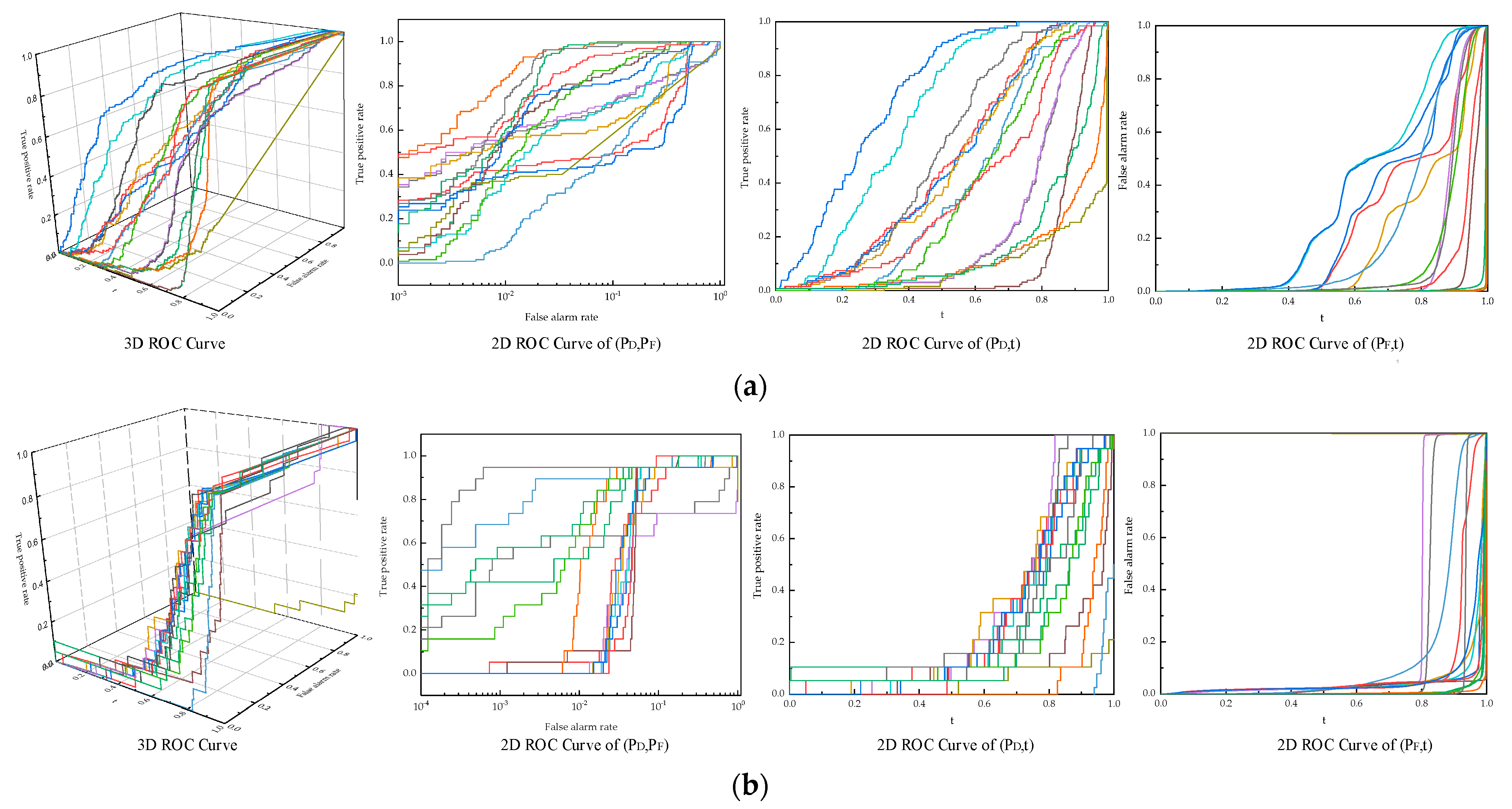
3.2.2. Evaluation Criteria
3.3. Experimental Results for Feature Extraction
3.4. Experimental Results for KMNF-BSM-Based Methods
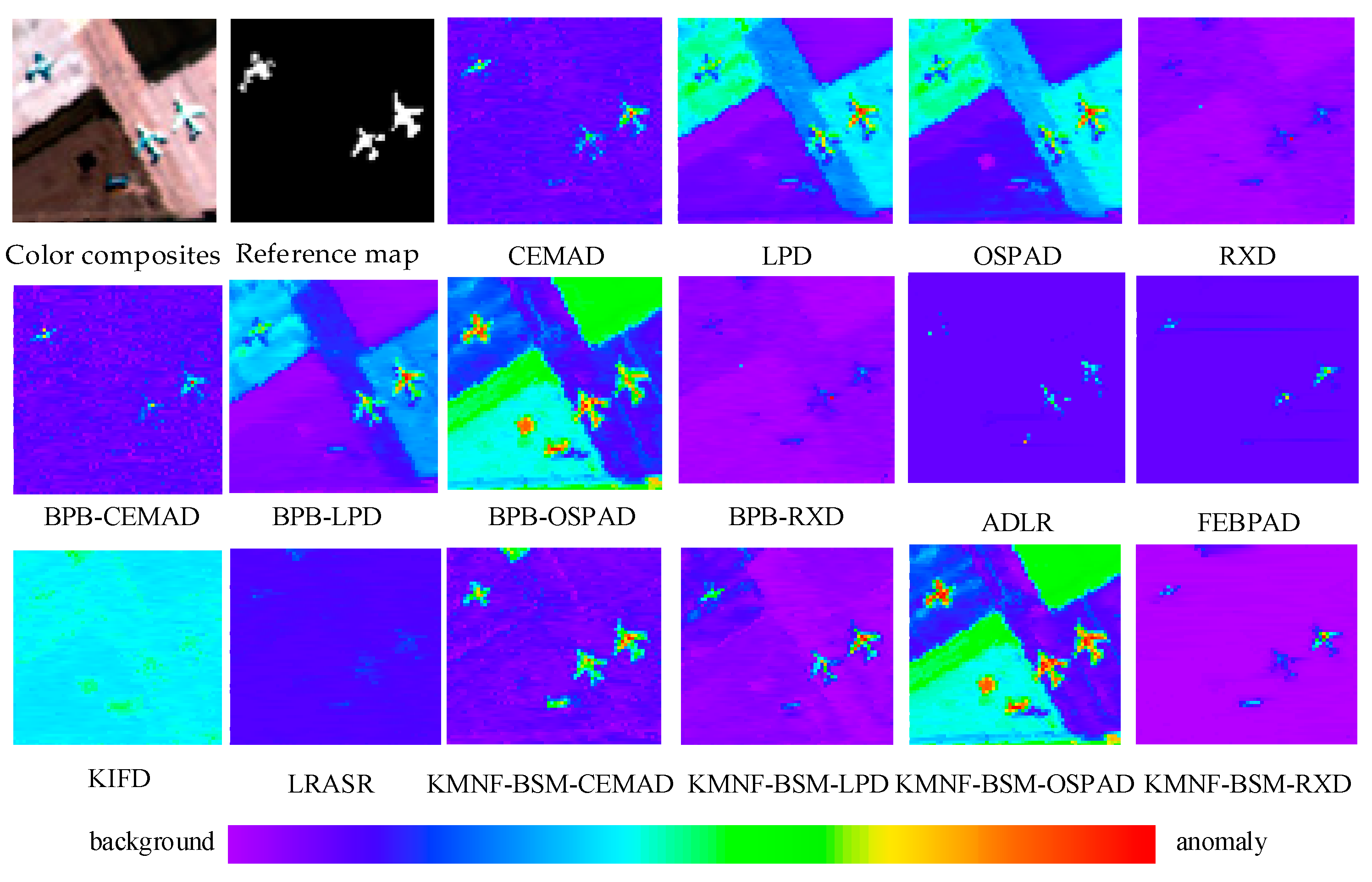
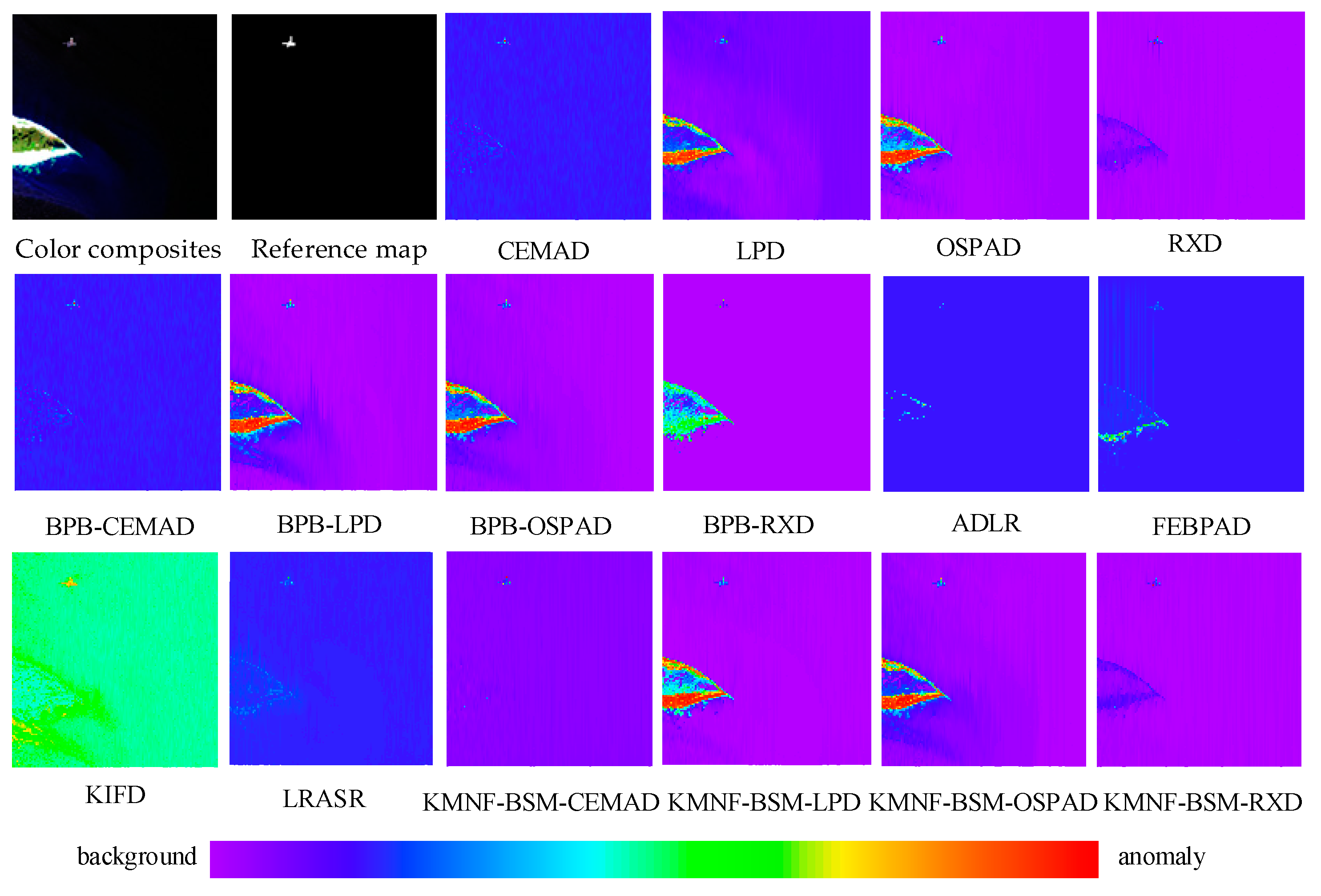
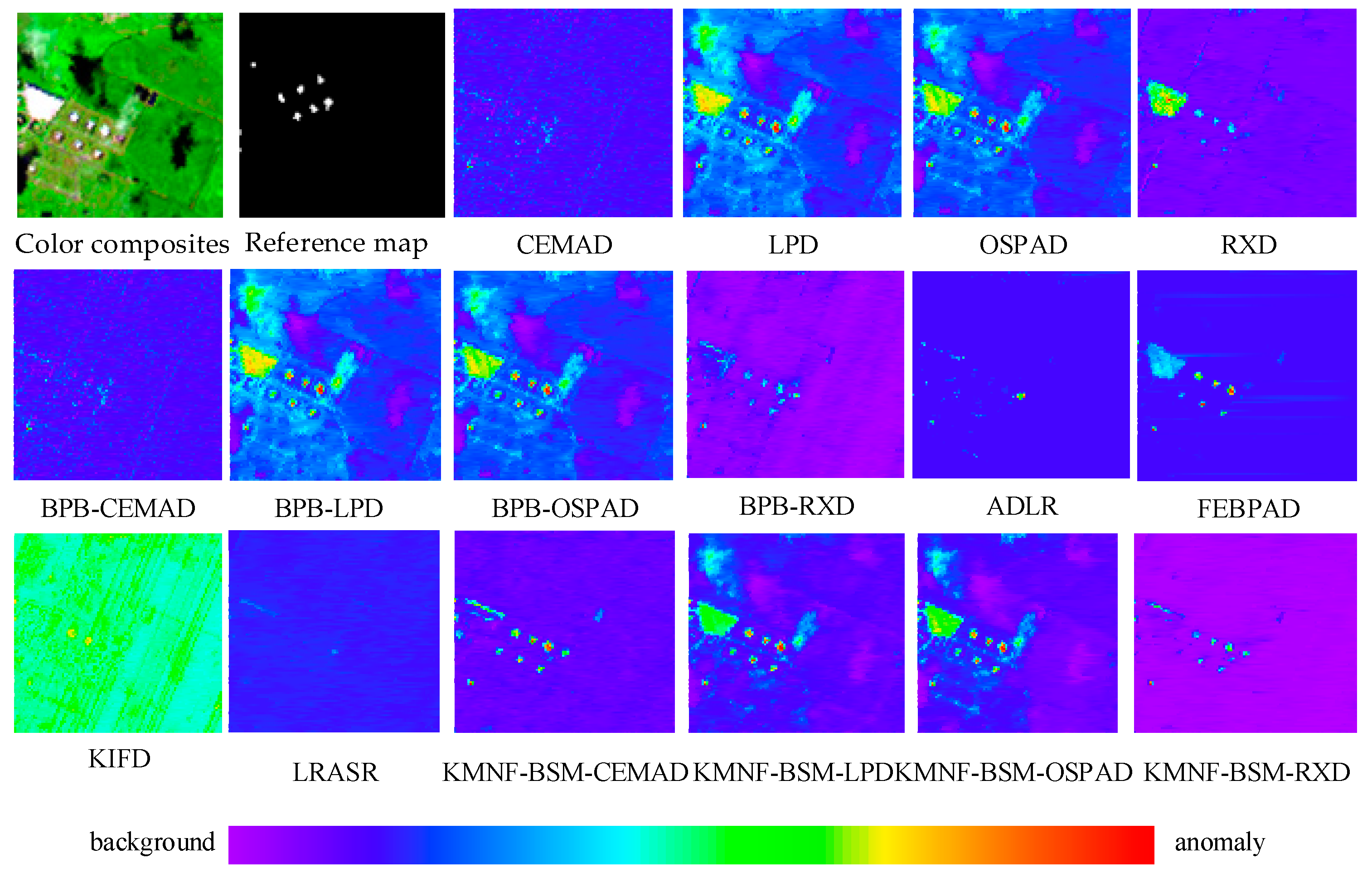
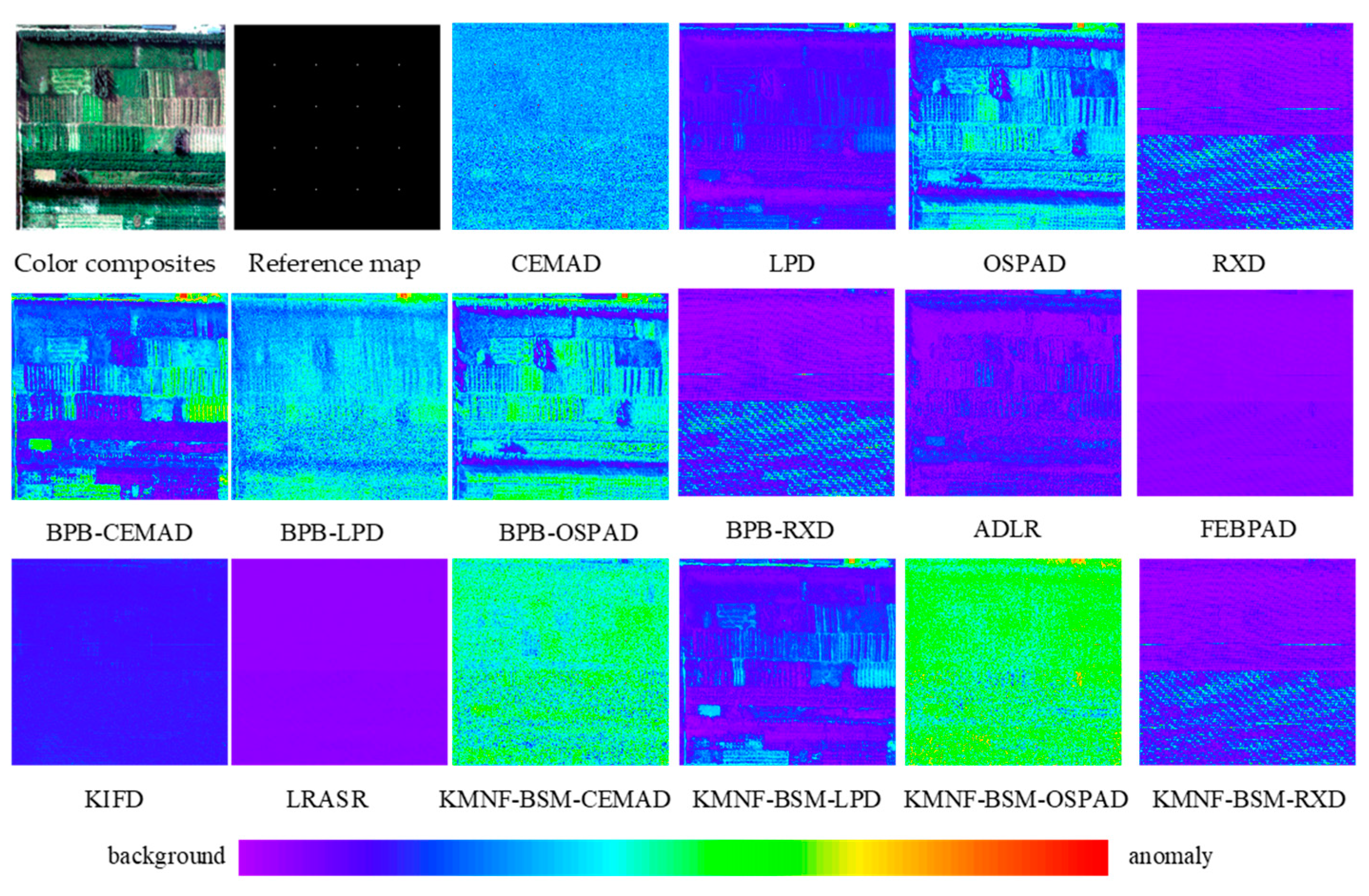
3.4.1. KMNF-BSM-Based Methods for HSIs over Different Scenes
3.4.2. KMNF-BSM-Based Methods for HSIs under Different Noise Levels
3.4.3. KMNF-BSM-Based Methods for HSIs with Different Spatial and Spectral Resolutions
4. Discussion
5. Conclusions
- (1)
- Taking the high-order correlation between spectral bands in HSIs into account, the detection ability of various feature extraction methods (including LDA, PCA, MNF, OMNF, FA, KPCA, OKMNF, LPP, LLE, and KMNF) in AD is evaluated in this article. The results illustrate that the KMNF transformation is more effective and robust in feature extraction for AD than other methods, providing a reference for further research on feature extraction in AD.
- (2)
- When the abnormal pixels occupy a small portion of the entire image, there will be little influence of the anomalies on background estimation, and the deviation between the estimated and true backgrounds will be minor.
- (3)
- Aiming to separate anomalies and background efficiently, a BSM that combines the outlier removal, the iteration strategy, and the RXD is proposed in this article. The results show that the KMNF-BSM has significant anti-noise ability and adaptability to HSIs with different spatial and spectral resolutions.
Author Contributions
Funding
Data Availability Statement
Acknowledgments
Conflicts of Interest
References
- Du, B.; Zhang, L. Random-Selection-Based Anomaly Detector for Hyperspectral Imagery. IEEE Trans. Geosci. Remote Sens. 2011, 49, 1578–1589. [Google Scholar] [CrossRef]
- Shaw, G.; Manolakis, D. Signal processing for hyperspectral image exploitation. IEEE Signal Process. Mag. 2002, 19, 12–16. [Google Scholar] [CrossRef]
- Landgrebe, D. Hyperspectral image data analysis. IEEE Signal Process. Mag. 2002, 19, 17–28. [Google Scholar] [CrossRef]
- Zhang, Y.; Du, B.; Zhang, L.; Wang, S. A Low-Rank and Sparse Matrix Decomposition-Based Mahalanobis Distance Method for Hyperspectral Anomaly Detection. IEEE Trans. Geosci. Remote Sens. 2016, 54, 1376–1389. [Google Scholar] [CrossRef]
- Sun, W.; Ren, K.; Meng, X.; Yang, G.; Xiao, C.; Peng, J.; Huang, J. MLR-DBPFN: A Multi-Scale Low Rank Deep Back Projection Fusion Network for Anti-Noise Hyperspectral and Multispectral Image Fusion. IEEE Trans. Geosci. Remote Sens. 2022, 60, 1–14. [Google Scholar] [CrossRef]
- Sun, W.; Yang, G.; Peng, J.; Meng, X.; He, K.; Li, W.; Li, H.; Du, Q. A Multiscale Spectral Features Graph Fusion Method for Hyperspectral Band Selection. IEEE Trans. Geosci. Remote Sens. 2022, 60, 1–12. [Google Scholar] [CrossRef]
- Kang, X.; Zhang, X.; Li, S.; Li, K.; Li, J.; Benediktsson, J.A. Hyperspectral Anomaly Detection with Attribute and Edge-Preserving Filters. IEEE Trans. Geosci. Remote Sens. 2017, 55, 5600–5611. [Google Scholar] [CrossRef]
- Manolakis, D.; Shaw, G. Detection algorithms for hyperspectral imaging applications. IEEE Signal Process. Mag. 2002, 19, 29–43. [Google Scholar] [CrossRef]
- Stein, D.W.J.; Beaven, S.G.; Hoff, L.E.; Winter, E.M.; Schaum, A.P.; Stocker, A.D. Anomaly detection from hyperspectral imagery. IEEE Signal Process. Mag. 2002, 19, 58–69. [Google Scholar] [CrossRef] [Green Version]
- Chang, C.I.; Chiang, S.S. Anomaly detection and classification for hyperspectral imagery. IEEE Trans. Geosci. Remote Sens. 2002, 40, 1314–1325. [Google Scholar] [CrossRef]
- Sun, X.; Zhang, B.; Zhuang, L.; Gao, H.; Sun, X.; Ni, L. Anomaly Detection Based on Tree Topology for Hyperspectral Images. IEEE J. Sel. Top. Appl. Earth Obs. Remote Sens. 2022. early access. [Google Scholar] [CrossRef]
- Fan, G.; Ma, Y.; Mei, X.; Fan, F.; Huang, J.; Ma, J. Hyperspectral Anomaly Detection with Robust Graph Autoencoders. IEEE Trans. Geosci. Remote Sens. 2022, 60, 1–14. [Google Scholar] [CrossRef]
- Rao, W.; Gao, L.; Qu, Y.; Sun, X.; Zhang, B.; Jocelyn, C. Siamese Transformer Network for Hyperspectral Image Target Detection. IEEE Trans. Geosci. Remote Sens. 2022, 60, 1–19. [Google Scholar] [CrossRef]
- Rao, W.; Qu, Y.; Gao, L.; Sun, X.; Wu, Y.; Zhang, B. Transferable network with Siamese architecture for anomaly detection in hyperspectral images. Int. J. Appl. Earth Obs. Geoinf. 2022, 106, 102669. [Google Scholar] [CrossRef]
- Zhao, R.; Du, B.; Zhang, L.; Zhang, L. A robust background regression-based score estimation algorithm for hyperspectral anomaly detection. ISPRS J. Photogramm. Remote Sens. 2016, 122, 126–144. [Google Scholar] [CrossRef]
- Matteoli, S.; Veracini, T.; Diani, M.; Corsini, G. Models and Methods for Automated Background Density Estimation in Hyperspectral Anomaly Detection. IEEE Trans. Geosci. Remote Sens. 2013, 51, 2837–2852. [Google Scholar] [CrossRef]
- Reed, I.S.; Yu, X. Adaptive multiple-band CFAR detection of an optical pattern with unknown spectral distribution. IEEE Trans. Signal Process. 1990, 38, 1760–1770. [Google Scholar] [CrossRef]
- Kwon, H.; Nasrabadi, N.M. Kernel RX-algorithm: A nonlinear anomaly detector for hyperspectral imagery. IEEE Trans. Geosci. Remote Sens. 2005, 43, 388–397. [Google Scholar] [CrossRef]
- Carlotto, M.J. A cluster-based approach for detecting man-made objects and changes in imagery. IEEE Trans. Geosci. Remote Sens. 2005, 43, 374–387. [Google Scholar] [CrossRef]
- Schaum, A.P. Hyperspectral anomaly detection beyond RX. SPIE Proc. 2007, 6565, 1–13. [Google Scholar] [CrossRef]
- Gu, Y.; Liu, Y.; Zhang, Y. A Selective KPCA Algorithm Based on High-Order Statistics for Anomaly Detection in Hyperspectral Imagery. IEEE Geosci. Remote Sens. Lett. 2008, 5, 43–47. [Google Scholar] [CrossRef]
- Zhang, Y.; Fan, Y.; Xu, M. A Background-Purification-Based Framework for Anomaly Target Detection in Hyperspectral Imagery. IEEE Geosci. Remote Sens. Lett. 2020, 17, 1238–1242. [Google Scholar] [CrossRef]
- Zhong, J.; Xie, W.; Li, Y.; Lei, J.; Du, Q. Characterization of Background-Anomaly Separability with Generative Adversarial Network for Hyperspectral Anomaly Detection. IEEE Trans. Geosci. Remote Sens. 2021, 59, 6017–6028. [Google Scholar] [CrossRef]
- Wang, S.; Wang, X.; Zhang, L.; Zhong, Y. Auto-AD: Autonomous Hyperspectral Anomaly Detection Network Based on Fully Convolutional Autoencoder. IEEE Trans. Geosci. Remote Sens. 2022, 60, 1–14. [Google Scholar] [CrossRef]
- Sun, X.; Qu, Y.; Gao, L.; Sun, X.; Qi, H.; Zhang, B.; Shen, T. Target Detection Through Tree-Structured Encoding for Hyperspectral Images. IEEE Trans. Geosci. Remote Sens. 2021, 59, 4233–4249. [Google Scholar] [CrossRef]
- Su, H.; Wu, Z.; Du, Q.; Du, P. Hyperspectral Anomaly Detection Using Collaborative Representation with Outlier Removal. IEEE J. Sel. Top. Appl. Earth Obs. Remote Sens. 2018, 11, 5029–5038. [Google Scholar] [CrossRef]
- Zhao, C.; Wang, X.; Yao, X.; Tian, M. A background refinement method based on local density for hyperspectral anomaly detection. J. Cent. South Univ. 2018, 25, 84–94. [Google Scholar] [CrossRef]
- Vafadar, M.; Ghassemian, H. Anomaly Detection of Hyperspectral Imagery Using Modified Collaborative Representation. IEEE Geosci. Remote Sens. Lett. 2018, 15, 577–581. [Google Scholar] [CrossRef]
- Gao, L.; Guo, Q.; Plaza Antonio, J.; Li, J.; Zhang, B. Probabilistic anomaly detector for remotely sensed hyperspectral data. J. Appl. Remote Sens. 2014, 8, 083538. [Google Scholar] [CrossRef]
- Billor, N.; Hadi Ali, S.; Velleman Paul, F. BACON: Blocked adaptive computationally efficient outlier nominators. Comput. Stat. Data Anal. 2000, 34, 279–298. [Google Scholar] [CrossRef]
- Taitano, Y.P.; Geier, B.A.; Bauer, K.W., Jr. A Locally Adaptable Iterative RX Detector. EURASIP J. Adv. Signal Process. 2010, 2010, 341908. [Google Scholar] [CrossRef] [Green Version]
- Sun, X.; Qu, Y.; Gao, L.; Sun, X.; Qi, H.; Zhang, B.; Shen, T. Ensemble-Based Information Retrieval with Mass Estimation for Hyperspectral Target Detection. IEEE Trans. Geosci. Remote Sens. 2022, 60, 1–23. [Google Scholar] [CrossRef]
- Dong, Y.; Du, B.; Zhang, L.; Zhang, L. Dimensionality Reduction and Classification of Hyperspectral Images Using Ensemble Discriminative Local Metric Learning. IEEE Trans. Geosci. Remote Sens. 2017, 55, 2509–2524. [Google Scholar] [CrossRef]
- Nielsen, A.A. Kernel Maximum Autocorrelation Factor and Minimum Noise Fraction Transformations. IEEE Trans. Image Process. 2011, 20, 612–624. [Google Scholar] [CrossRef] [PubMed] [Green Version]
- Xie, W.; Fan, S.; Qu, J.; Wu, X.; Lu, Y.; Du, Q. Spectral Distribution-Aware Estimation Network for Hyperspectral Anomaly Detection. IEEE Trans. Geosci. Remote Sens. 2022, 60, 1–12. [Google Scholar] [CrossRef]
- Robila, S.A.; Gershman, A. Spectral Matching Accuracy in Processing Hyperspectral Data. In Proceedings of the International Symposium on Signals Circuits and Systems, Iasi, Romania, 14–15 July 2005. [Google Scholar] [CrossRef]
- Xie, W.; Li, Y.; Lei, J.; Yang, J.; Chang, C.; Li, Z. Hyperspectral Band Selection for Spectral–Spatial Anomaly Detection. IEEE Trans. Geosci. Remote Sens. 2020, 58, 3426–3436. [Google Scholar] [CrossRef]
- Harsanyi, J.C. Detection and Classification of Subpixel Spectral Signatures in Hyperspectral Image Sequences. Ph.D. Thesis, Department of Electronic & Electrical Engineering, University of Maryland Baltimore County, Baltimore, MD, USA, 1993. [Google Scholar]
- Harsanyi, J.C.; Chang, C.-I. Hyperspectral image classification and dimensionality reduction: An orthogonal subspace projection approach. IEEE Trans. Geosci. Remote Sens. 1994, 32, 779–785. [Google Scholar] [CrossRef] [Green Version]
- Chang, C.-I.; Heinz, D.C. Constrained subpixel target detection for remotely sensed imagery. IEEE Trans. Geosci. Remote Sens. 2000, 38, 1144–1159. [Google Scholar] [CrossRef] [Green Version]
- Qu, Y.; Wang, W.; Guo, R.; Ayhan, B.; Kwan, C.; Vance, S.; Qi, H. Hyperspectral Anomaly Detection Through Spectral Unmixing and Dictionary-Based Low-Rank Decomposition. IEEE Trans. Geosci. Remote Sens. 2018, 56, 4391–4405. [Google Scholar] [CrossRef]
- Xu, Y.; Wu, Z.; Li, J.; Plaza, A.; Wei, Z. Anomaly Detection in Hyperspectral Images Based on Low-Rank and Sparse Representation. IEEE Trans. Geosci. Remote Sens. 2016, 54, 1990–2000. [Google Scholar] [CrossRef]
- Ma, Y.; Fan, G.; Jin, Q.; Huang, J.; Mei, X.; Ma, J. Hyperspectral Anomaly Detection via Integration of Feature Extraction and Background Purification. IEEE Geosci. Remote Sens. Lett. 2021, 18, 1436–1440. [Google Scholar] [CrossRef]
- Li, S.; Zhang, K.; Duan, P.; Kang, X. Hyperspectral Anomaly Detection with Kernel Isolation Forest. IEEE Trans. Geosci. Remote Sens. 2020, 58, 319–329. [Google Scholar] [CrossRef]
- Zou, Z.; Shi, Z. Hierarchical Suppression Method for Hyperspectral Target Detection. IEEE Trans. Geosci. Remote Sens. 2016, 54, 330–342. [Google Scholar] [CrossRef]
- Li, Z.; Zhang, Y. Hyperspectral Anomaly Detection via Image Super-Resolution Processing and Spatial Correlation. IEEE Trans. Geosci. Remote Sens. 2021, 59, 2307–2320. [Google Scholar] [CrossRef]
- Jia, J.; Wang, Y.; Cheng, X.; Yuan, L.; Zhao, D.; Ye, Q.; Zhuang, X.; Shu, R.; Wang, J. Destriping Algorithms Based on Statistics and Spatial Filtering for Visible-to-Thermal Infrared Pushbroom Hyperspectral Imagery. IEEE Trans. Geosci. Remote Sens. 2019, 57, 4077–4091. [Google Scholar] [CrossRef]
- Jia, J.; Zheng, X.; Guo, S.; Wang, Y.; Chen, J. Removing Stripe Noise Based on Improved Statistics for Hyperspectral Images. IEEE Geosci. Remote Sens. Lett. 2022, 19, 1–5. [Google Scholar] [CrossRef]
- Xue, T.; Wang, Y.; Chen, Y.; Jia, J.; Wen, M.; Guo, R.; Wu, T.; Deng, X. Mixed Noise Estimation Model for Optimized Kernel Minimum Noise Fraction Transformation in Hyperspectral Image Dimensionality Reduction. Remote Sens. 2021, 13, 2607. [Google Scholar] [CrossRef]
- Jia, J.; Chen, J.; Zheng, X.; Wang, Y.; Guo, S.; Sun, H.; Jiang, C.; Karjalainen, M.; Karila, K.; Duan, Z.; et al. Tradeoffs in the Spatial and Spectral Resolution of Airborne Hyperspectral Imaging Systems: A Crop Identification Case Study. IEEE Trans. Geosci. Remote Sens. 2022, 60, 1–18. [Google Scholar] [CrossRef]
- Chang, C.I. An Effective Evaluation Tool for Hyperspectral Target Detection: 3D Receiver Operating Characteristic Curve Analysis. IEEE Trans. Geosci. Remote Sens. 2021, 59, 5131–5153. [Google Scholar] [CrossRef]


| Methods | CEMAD | LPD | OSPAD | RXD | Average | Standard Deviation |
|---|---|---|---|---|---|---|
| airport scene | ||||||
| None | 0.857013 | 0.811844 | 0.772991 | 0.957333 | 0.849795 | 0.068840 |
| FA | 0.705287 | 0.677984 | 0.599139 | 0.984278 | 0.741672 | 0.145390 |
| KPCA | 0.729342 | 0.867161 | 0.779185 | 0.975777 | 0.837866 | 0.093673 |
| LDA | 0.620843 | 0.664756 | 0.816110 | 0.978925 | 0.770158 | 0.140623 |
| LLE | 0.701738 | 0.576013 | 0.843780 | 0.977550 | 0.774770 | 0.150599 |
| LPP | 0.729904 | 0.681332 | 0.764991 | 0.976652 | 0.788220 | 0.112774 |
| MNF | 0.715573 | 0.628473 | 0.978940 | 0.983811 | 0.826699 | 0.157721 |
| OKMNF | 0.542965 | 0.983694 | 0.517016 | 0.983252 | 0.756732 | 0.226927 |
| OMNF | 0.579210 | 0.501744 | 0.989940 | 0.984292 | 0.763797 | 0.225002 |
| PCA | 0.602021 | 0.650877 | 0.569776 | 0.970020 | 0.698174 | 0.159584 |
| KMNF | 0.877646 | 0.932705 | 0.929443 | 0.981390 | 0.930296 | 0.036705 |
| beach scene | ||||||
| None | 0.819380 | 0.910611 | 0.909312 | 0.976638 | 0.903985 | 0.055921 |
| FA | 0.921028 | 0.552103 | 0.967202 | 0.980385 | 0.855180 | 0.176364 |
| KPCA | 0.902115 | 0.963578 | 0.945545 | 0.953594 | 0.941208 | 0.023457 |
| LDA | 0.907913 | 0.737984 | 0.724724 | 0.961316 | 0.832984 | 0.103475 |
| LLE | 0.943337 | 0.927826 | 0.932625 | 0.950857 | 0.938661 | 0.009006 |
| LPP | 0.981773 | 0.920338 | 0.933602 | 0.931036 | 0.941687 | 0.023672 |
| MNF | 0.943531 | 0.829997 | 0.622944 | 0.966967 | 0.840860 | 0.136060 |
| OKMNF | 0.738756 | 0.950395 | 0.937530 | 0.942007 | 0.892172 | 0.088695 |
| OMNF | 0.837243 | 0.702620 | 0.707177 | 0.966893 | 0.803483 | 0.108732 |
| PCA | 0.884658 | 0.724257 | 0.922945 | 0.955794 | 0.871914 | 0.088889 |
| KMNF | 0.945130 | 0.920347 | 0.939727 | 0.977237 | 0.945610 | 0.020453 |
| urban scene | ||||||
| None | 0.667807 | 0.979568 | 0.985286 | 0.949350 | 0.895503 | 0.132167 |
| FA | 0.981016 | 0.635529 | 0.560354 | 0.989976 | 0.791719 | 0.195617 |
| KPCA | 0.982866 | 0.537097 | 0.972700 | 0.990535 | 0.870800 | 0.192767 |
| LDA | 0.860412 | 0.956259 | 0.986726 | 0.990576 | 0.948493 | 0.052563 |
| LLE | 0.992927 | 0.960108 | 0.799670 | 0.991776 | 0.936120 | 0.079873 |
| LPP | 0.905048 | 0.983349 | 0.984986 | 0.991155 | 0.966135 | 0.035388 |
| MNF | 0.981934 | 0.822225 | 0.989893 | 0.991946 | 0.946500 | 0.071847 |
| OKMNF | 0.981582 | 0.986586 | 0.904523 | 0.991493 | 0.966046 | 0.035693 |
| OMNF | 0.888050 | 0.680471 | 0.991122 | 0.991974 | 0.887904 | 0.126997 |
| PCA | 0.983820 | 0.949867 | 0.975597 | 0.980033 | 0.972329 | 0.013291 |
| KMNF | 0.946366 | 0.983100 | 0.986795 | 0.991328 | 0.976897 | 0.017866 |
| vegetation scene | ||||||
| None | 0.999992 | 0.599149 | 0.592237 | 0.644218 | 0.708881 | 0.169246 |
| FA | 0.999816 | 0.848157 | 0.706734 | 0.951344 | 0.876513 | 0.123557 |
| KPCA | 0.998871 | 0.516278 | 0.655223 | 0.998518 | 0.792223 | 0.161827 |
| LDA | 0.993730 | 0.687711 | 0.641945 | 1.000000 | 0.830847 | 0.153623 |
| LLE | 0.996232 | 0.603171 | 0.649694 | 0.999624 | 0.812180 | 0.194088 |
| LPP | 0.998282 | 0.547374 | 0.658815 | 0.999549 | 0.801005 | 0.184973 |
| MNF | 0.999816 | 0.531912 | 0.853890 | 0.951344 | 0.834241 | 0.142195 |
| OKMNF | 0.991259 | 0.710232 | 0.627005 | 1.000000 | 0.832124 | 0.146672 |
| OMNF | 0.999800 | 0.671591 | 0.920110 | 0.957493 | 0.887249 | 0.164683 |
| PCA | 0.984193 | 0.522218 | 0.734254 | 1.000000 | 0.810166 | 0.189983 |
| KMNF | 0.999706 | 0.842263 | 0.767805 | 0.974503 | 0.896069 | 0.148757 |
| Methods | |||||||||
|---|---|---|---|---|---|---|---|---|---|
| airport scene | |||||||||
| CEMAD | 0.85701 | 0.23338 | 0.11346 | 1.09039 | 0.74355 | 0.11992 | 1.11992 | 0.97693 | 2.05690 |
| LPD | 0.81184 | 0.36868 | 0.23769 | 1.18053 | 0.57416 | 0.13100 | 1.13100 | 0.94284 | 1.55114 |
| OSPAD | 0.77299 | 0.47182 | 0.37399 | 1.24481 | 0.39900 | 0.09783 | 1.09783 | 0.87082 | 1.26158 |
| RXD | 0.95735 | 0.12820 | 0.03944 | 1.08554 | 0.91790 | 0.08875 | 1.08875 | 1.04610 | 3.25005 |
| BPB-CEMAD | 0.85768 | 0.23599 | 0.11299 | 1.09367 | 0.74469 | 0.12300 | 1.12300 | 0.98068 | 2.08856 |
| BPB-LPD | 0.88211 | 0.46088 | 0.17553 | 1.34300 | 0.70658 | 0.28535 | 1.28535 | 1.16746 | 2.62561 |
| BPB-OSPAD | 0.90440 | 0.65398 | 0.34849 | 1.55838 | 0.55591 | 0.30549 | 1.30549 | 1.20989 | 1.87662 |
| BPB-RXD | 0.95743 | 0.12831 | 0.03949 | 1.08575 | 0.91794 | 0.08882 | 1.08882 | 1.04626 | 3.24911 |
| ADLR | 0.60125 | 0.09063 | 0.03612 | 0.69187 | 0.56513 | 0.05451 | 1.05451 | 0.65576 | 2.50925 |
| FEBPAD | 0.97401 | 0.12430 | 0.30069 | 1.09831 | 0.67332 | −0.17640 | 0.82360 | 0.79761 | 0.41336 |
| KIFD | 0.80077 | 0.38660 | 0.22219 | 1.18737 | 0.57858 | 0.16441 | 1.16441 | 0.96518 | 1.73992 |
| LRASR | 0.95722 | 0.36527 | 0.10914 | 1.32249 | 0.84808 | 0.25613 | 1.25613 | 1.21335 | 3.34679 |
| KMNF-BSM-CEMAD | 0.98811 | 0.51859 | 0.11299 | 1.50670 | 0.87512 | 0.40560 | 1.40560 | 1.39371 | 4.58971 |
| KMNF-BSM-LPD | 0.97164 | 0.48301 | 0.06069 | 1.45466 | 0.91095 | 0.42232 | 1.42232 | 1.39396 | 7.95840 |
| KMNF-BSM-OSPAD | 0.94197 | 0.73273 | 0.33245 | 1.67470 | 0.60952 | 0.40028 | 1.40028 | 1.34225 | 2.20401 |
| KMNF-BSM-RXD | 0.98797 | 0.16302 | 0.00783 | 1.15098 | 0.98014 | 0.15519 | 1.15519 | 1.14315 | 20.8249 |
| beach scene | |||||||||
| CEMAD | 0.81938 | 0.25592 | 0.17467 | 1.07530 | 0.64471 | 0.08125 | 1.08125 | 0.90063 | 1.46516 |
| LPD | 0.91061 | 0.28447 | 0.08998 | 1.19508 | 0.82064 | 0.19449 | 1.19449 | 1.10510 | 3.16160 |
| OSPAD | 0.90931 | 0.25479 | 0.05393 | 1.16410 | 0.85539 | 0.20087 | 1.20087 | 1.11018 | 4.72476 |
| RXD | 0.97664 | 0.18987 | 0.01218 | 1.16650 | 0.96446 | 0.17768 | 1.17768 | 1.15432 | 15.5857 |
| BPB-CEMAD | 0.71298 | 0.20172 | 0.21102 | 0.91470 | 0.50196 | −0.00930 | 0.99070 | 0.70368 | 0.95592 |
| BPB-LPD | 0.91889 | 0.26124 | 0.05088 | 1.18012 | 0.86801 | 0.21036 | 1.21036 | 1.12925 | 5.13484 |
| BPB-OSPAD | 0.94013 | 0.26540 | 0.04675 | 1.20553 | 0.89338 | 0.21865 | 1.21865 | 1.15877 | 5.67660 |
| BPB-RXD | 0.94783 | 0.11600 | 0.02073 | 1.06383 | 0.92710 | 0.09527 | 1.09527 | 1.04310 | 5.59472 |
| ADLR | 0.95980 | 0.25317 | 0.19913 | 1.21296 | 0.76067 | 0.05404 | 1.05404 | 1.01383 | 1.27138 |
| FEBPAD | 0.96310 | 0.06436 | 0.01504 | 1.02745 | 0.94805 | 0.04932 | 1.04932 | 1.01241 | 4.27862 |
| KIFD | 0.96029 | 0.22135 | 0.14216 | 1.18164 | 0.81813 | 0.07919 | 1.07919 | 1.03948 | 1.55701 |
| LRASR | 0.96518 | 0.20119 | 0.01063 | 1.16637 | 0.95455 | 0.19056 | 1.19056 | 1.15574 | 18.9302 |
| KMNF-BSM-CEMAD | 0.97923 | 0.26375 | 0.06463 | 1.24298 | 0.91460 | 0.19911 | 1.19911 | 1.17834 | 4.08078 |
| KMNF-BSM-LPD | 0.95503 | 0.30032 | 0.04065 | 1.25535 | 0.91438 | 0.25967 | 1.25967 | 1.21470 | 7.38800 |
| KMNF-BSM-OSPAD | 0.94628 | 0.27827 | 0.04302 | 1.22454 | 0.90326 | 0.23525 | 1.23525 | 1.18152 | 6.46832 |
| KMNF-BSM-RXD | 0.97844 | 0.25519 | 0.00896 | 1.23363 | 0.96948 | 0.24623 | 1.24623 | 1.22467 | 28.4683 |
| urban scene | |||||||||
| CEMAD | 0.66781 | 0.21341 | 0.15409 | 0.88122 | 0.51372 | 0.05933 | 1.05933 | 0.72713 | 1.38501 |
| LPD | 0.97957 | 0.62279 | 0.25043 | 1.60236 | 0.72914 | 0.37236 | 1.37236 | 1.35193 | 2.48687 |
| OSPAD | 0.98529 | 0.63414 | 0.20286 | 1.61943 | 0.78243 | 0.43128 | 1.43128 | 1.41657 | 3.12600 |
| RXD | 0.94935 | 0.28452 | 0.10287 | 1.23387 | 0.84649 | 0.18165 | 1.18165 | 1.13100 | 2.76595 |
| BPB-CEMAD | 0.66781 | 0.21341 | 0.15409 | 0.88122 | 0.51372 | 0.05933 | 1.05933 | 0.72713 | 1.38501 |
| BPB-LPD | 0.97946 | 0.64885 | 0.25042 | 1.62831 | 0.72904 | 0.39843 | 1.39843 | 1.37789 | 2.59107 |
| BPB-OSPAD | 0.98418 | 0.62330 | 0.22271 | 1.60749 | 0.76147 | 0.40059 | 1.40059 | 1.38477 | 2.79871 |
| BPB-RXD | 0.99055 | 0.29761 | 0.05551 | 1.28816 | 0.93504 | 0.24210 | 1.24210 | 1.23265 | 5.36121 |
| ADLR | 0.98638 | 0.97468 | 0.99819 | 1.96106 | −0.01181 | −0.02351 | 0.97649 | 0.96287 | 0.97645 |
| FEBPAD | 0.98957 | 0.36379 | 0.20587 | 1.35336 | 0.78371 | 0.15792 | 1.15792 | 1.14749 | 1.76711 |
| KIFD | 0.92620 | 0.56301 | 0.18608 | 1.48921 | 0.74012 | 0.37693 | 1.37693 | 1.30313 | 3.02565 |
| LRASR | 0.92157 | 0.25150 | 0.11350 | 1.17308 | 0.80807 | 0.13801 | 1.13801 | 1.05958 | 2.21595 |
| KMNF-BSM-CEMAD | 0.99568 | 0.56736 | 0.11788 | 1.56304 | 0.87780 | 0.44948 | 1.44948 | 1.44516 | 4.81306 |
| KMNF-BSM-LPD | 0.98702 | 0.64887 | 0.15471 | 1.63588 | 0.83230 | 0.49415 | 1.49415 | 1.48117 | 4.19399 |
| KMNF-BSM-OSPAD | 0.98554 | 0.63988 | 0.14765 | 1.62542 | 0.83789 | 0.49223 | 1.49223 | 1.47777 | 4.33370 |
| KMNF-BSM-RXD | 0.99455 | 0.31125 | 0.01637 | 1.30580 | 0.97818 | 0.29488 | 1.29488 | 1.28943 | 19.0112 |
| vegetation scene | |||||||||
| CEMAD | 0.99999 | 0.00951 | 0.00328 | 1.00950 | 0.99671 | 0.00622 | 1.00622 | 1.00622 | 2.89552 |
| LPD | 0.59915 | 0.00153 | 0.00172 | 0.60068 | 0.59743 | −0.00019 | 0.99981 | 0.59896 | 0.88773 |
| OSPAD | 0.59224 | 0.00287 | 0.00531 | 0.59511 | 0.58693 | −0.00244 | 0.99756 | 0.58979 | 0.54010 |
| RXD | 0.64422 | 0.00070 | 0.00873 | 0.64492 | 0.63549 | −0.00803 | 0.99197 | 0.63619 | 0.08040 |
| BPB-CEMAD | 0.82903 | 0.00395 | 0.00466 | 0.83299 | 0.82437 | −0.00071 | 0.99929 | 0.82832 | 0.84752 |
| BPB-LPD | 0.65499 | 0.00224 | 0.00371 | 0.65723 | 0.65128 | −0.00147 | 0.99853 | 0.65352 | 0.60475 |
| BPB-OSPAD | 0.62705 | 0.00317 | 0.00355 | 0.63022 | 0.62350 | −0.00038 | 0.99962 | 0.62667 | 0.89308 |
| BPB-RXD | 0.64449 | 0.00070 | 0.00140 | 0.64519 | 0.64309 | −0.00070 | 0.99930 | 0.64379 | 0.50215 |
| ADLR | 0.89237 | 0.87298 | 0.67413 | 1.56535 | 0.21824 | −0.00114 | 0.99886 | 0.89122 | 0.99830 |
| FEBPAD | 0.76463 | 0.98256 | 0.95604 | 1.64719 | −0.19141 | −0.07348 | 0.92652 | 0.69115 | 0.92314 |
| KIFD | 0.56599 | 0.07298 | 0.07842 | 0.63897 | 0.48757 | −0.00543 | 0.99457 | 0.56056 | 0.93072 |
| LRASR | 0.53350 | 0.15576 | 0.17173 | 0.68927 | 0.36177 | −0.01597 | 0.98403 | 0.51753 | 0.90701 |
| KMNF-BSM-CEMAD | 0.99999 | 0.01000 | 0.00272 | 1.00999 | 0.99728 | 0.00728 | 1.00728 | 1.00728 | 3.68004 |
| KMNF-BSM-LPD | 0.76146 | 0.00340 | 0.00147 | 0.76487 | 0.75999 | 0.00193 | 1.00193 | 0.76339 | 2.30868 |
| KMNF-BSM-OSPAD | 0.99236 | 0.00739 | 0.00310 | 0.99975 | 0.98927 | 0.00429 | 1.00429 | 0.99665 | 2.38457 |
| KMNF-BSM-RXD | 0.65128 | 0.00932 | 0.00140 | 0.66060 | 0.64988 | 0.00793 | 1.00793 | 0.65921 | 6.67837 |
| Methods | ||||
|---|---|---|---|---|
| airport scene | ||||
| CEMAD | 0.767827 | 0.790570 | 0.759692 | 0.759671 |
| LPD | 0.606174 | 0.832911 | 0.543871 | 0.820496 |
| OSPAD | 0.669310 | 0.730488 | 0.765806 | 0.702719 |
| RXD | 0.884361 | 0.816857 | 0.775624 | 0.756052 |
| BPB-CEMAD | 0.762927 | 0.790233 | 0.757526 | 0.759521 |
| BPB-LPD | 0.748734 | 0.793912 | 0.880478 | 0.585944 |
| BPB-OSPAD | 0.846208 | 0.780548 | 0.774155 | 0.761130 |
| BPB-RXD | 0.879588 | 0.818812 | 0.778605 | 0.761802 |
| ADLR | 0.909785 | 0.910524 | 0.901263 | 0.901627 |
| FEBPAD | 0.986912 | 0.870969 | 0.945351 | 0.811967 |
| KIFD | 0.500462 | 0.519817 | 0.510212 | 0.579373 |
| LRASR | 0.763437 | 0.615707 | 0.549777 | 0.517181 |
| KMNF-BSM-CEMAD | 0.989317 | 0.843223 | 0.984707 | 0.982325 |
| KMNF-BSM-LPD | 0.810241 | 0.845787 | 0.946299 | 0.927393 |
| KMNF-BSM-OSPAD | 0.940265 | 0.857312 | 0.833355 | 0.783766 |
| KMNF-BSM-RXD | 0.981749 | 0.976846 | 0.962301 | 0.942672 |
| beach scene | ||||
| CEMAD | 0.733025 | 0.692576 | 0.672832 | 0.650229 |
| LPD | 0.932182 | 0.855841 | 0.819975 | 0.756692 |
| OSPAD | 0.934462 | 0.806198 | 0.721337 | 0.651162 |
| RXD | 0.822426 | 0.596543 | 0.590686 | 0.620596 |
| BPB-CEMAD | 0.725357 | 0.692724 | 0.673263 | 0.649206 |
| BPB-LPD | 0.659594 | 0.604609 | 0.863936 | 0.508946 |
| BPB-OSPAD | 0.937215 | 0.914567 | 0.886446 | 0.853600 |
| BPB-RXD | 0.834081 | 0.514230 | 0.683375 | 0.587055 |
| ADLR | 0.923657 | 0.928683 | 0.916493 | 0.912059 |
| FEBPAD | 0.934440 | 0.932733 | 0.926787 | 0.931915 |
| KIFD | 0.942347 | 0.929327 | 0.930814 | 0.934508 |
| LRASR | 0.936923 | 0.933985 | 0.903125 | 0.867168 |
| KMNF-BSM-CEMAD | 0.932935 | 0.840578 | 0.866664 | 0.911052 |
| KMNF-BSM-LPD | 0.943535 | 0.919491 | 0.929542 | 0.891736 |
| KMNF-BSM-OSPAD | 0.938193 | 0.934819 | 0.936318 | 0.936855 |
| KMNF-BSM-RXD | 0.897480 | 0.658520 | 0.874630 | 0.889253 |
| urban scene | ||||
| CEMAD | 0.879689 | 0.890308 | 0.889516 | 0.871628 |
| LPD | 0.986192 | 0.974899 | 0.915606 | 0.927822 |
| OSPAD | 0.981546 | 0.900978 | 0.975862 | 0.760433 |
| RXD | 0.952765 | 0.941403 | 0.934829 | 0.929170 |
| BPB-CEMAD | 0.883609 | 0.890197 | 0.889019 | 0.871261 |
| BPB-LPD | 0.739033 | 0.500289 | 0.908795 | 0.536912 |
| BPB-OSPAD | 0.985485 | 0.949995 | 0.983059 | 0.971710 |
| BPB-RXD | 0.953275 | 0.941261 | 0.934651 | 0.929149 |
| ADLR | 0.903738 | 0.915074 | 0.906458 | 0.904263 |
| FEBPAD | 0.946501 | 0.982272 | 0.929108 | 0.938624 |
| KIFD | 0.970845 | 0.966343 | 0.976179 | 0.976014 |
| LRASR | 0.923020 | 0.707483 | 0.782628 | 0.800433 |
| KMNF-BSM-CEMAD | 0.982947 | 0.986891 | 0.985046 | 0.988811 |
| KMNF-BSM-LPD | 0.990061 | 0.986862 | 0.938982 | 0.984113 |
| KMNF-BSM-OSPAD | 0.986395 | 0.987543 | 0.983330 | 0.987581 |
| KMNF-BSM-RXD | 0.974875 | 0.975066 | 0.978667 | 0.968654 |
| vegetation scene | ||||
| CEMAD | 0.610996 | 0.545534 | 0.523083 | 0.522589 |
| LPD | 0.521942 | 0.523286 | 0.532123 | 0.513940 |
| OSPAD | 0.591975 | 0.590166 | 0.571438 | 0.595121 |
| RXD | 0.534127 | 0.525701 | 0.524149 | 0.518445 |
| BPB-CEMAD | 0.611782 | 0.545564 | 0.522680 | 0.522766 |
| BPB-LPD | 0.503018 | 0.513404 | 0.510923 | 0.503790 |
| BPB-OSPAD | 0.591451 | 0.519143 | 0.559367 | 0.609736 |
| BPB-RXD | 0.534932 | 0.526477 | 0.524221 | 0.518689 |
| ADLR | 0.613593 | 0.614239 | 0.602584 | 0.601359 |
| FEBPAD | 0.625441 | 0.617946 | 0.584923 | 0.573634 |
| KIFD | 0.513805 | 0.577906 | 0.560019 | 0.510556 |
| LRASR | 0.533473 | 0.510411 | 0.507596 | 0.513850 |
| KMNF-BSM-CEMAD | 0.888332 | 0.619983 | 0.590621 | 0.531612 |
| KMNF-BSM-LPD | 0.584435 | 0.636560 | 0.713470 | 0.565725 |
| KMNF-BSM-OSPAD | 0.660492 | 0.692482 | 0.690609 | 0.666776 |
| KMNF-BSM-RXD | 0.563361 | 0.705072 | 0.672863 | 0.596751 |
| Methods | Spatial1 | Spatial2 | Spatial3 |
|---|---|---|---|
| CEMAD | 0.999992 | 0.986571 | 0.957254 |
| LPD | 0.599149 | 0.543385 | 0.605616 |
| OSPAD | 0.592237 | 0.633003 | 0.599736 |
| RXD | 0.644218 | 0.550181 | 0.624800 |
| BPB-CEMAD | 0.829034 | 0.986659 | 0.957718 |
| BPB-LPD | 0.654985 | 0.636896 | 0.559173 |
| BPB-OSPAD | 0.627050 | 0.601565 | 0.532161 |
| BPB-RXD | 0.644485 | 0.549245 | 0.624319 |
| ADLR | 0.892366 | 0.856324 | 0.802396 |
| FEBPAD | 0.764630 | 0.704130 | 0.613324 |
| KIFD | 0.565988 | 0.511737 | 0.942766 |
| LRASR | 0.533504 | 0.548252 | 0.556380 |
| KMNF-BSM-CEMAD | 0.999992 | 0.997604 | 0.963849 |
| KMNF-BSM-LPD | 0.761462 | 0.639630 | 0.610452 |
| KMNF-BSM-OSPAD | 0.992362 | 0.717830 | 0.603370 |
| KMNF-BSM-RXD | 0.651286 | 0.626007 | 0.715264 |
| Methods | Spectral1 | Spectral2 | Spectral3 |
|---|---|---|---|
| CEMAD | 0.999992 | 0.999996 | 0.999992 |
| LPD | 0.599149 | 0.756851 | 0.561840 |
| OSPAD | 0.592237 | 0.633389 | 0.797157 |
| RXD | 0.644218 | 0.652756 | 0.578054 |
| BPB-CEMAD | 0.829034 | 0.999996 | 0.999992 |
| BPB-LPD | 0.654985 | 0.793947 | 0.515565 |
| BPB-OSPAD | 0.627050 | 0.542546 | 0.544691 |
| BPB-RXD | 0.644485 | 0.652439 | 0.578836 |
| ADLR | 0.892366 | 0.865326 | 0.886534 |
| FEBPAD | 0.764630 | 0.695951 | 0.710523 |
| KIFD | 0.565988 | 0.556626 | 0.652714 |
| LRASR | 0.533504 | 0.569881 | 0.588985 |
| KMNF-BSM-CEMAD | 0.999992 | 0.999996 | 0.999996 |
| KMNF-BSM-LPD | 0.761462 | 0.982546 | 0.701198 |
| KMNF-BSM-OSPAD | 0.992362 | 0.650748 | 0.626065 |
| KMNF-BSM-RXD | 0.651286 | 0.734263 | 0.703591 |
Publisher’s Note: MDPI stays neutral with regard to jurisdictional claims in published maps and institutional affiliations. |
© 2022 by the authors. Licensee MDPI, Basel, Switzerland. This article is an open access article distributed under the terms and conditions of the Creative Commons Attribution (CC BY) license (https://creativecommons.org/licenses/by/4.0/).
Share and Cite
Xue, T.; Jia, J.; Xie, H.; Zhang, C.; Deng, X.; Wang, Y. Kernel Minimum Noise Fraction Transformation-Based Background Separation Model for Hyperspectral Anomaly Detection. Remote Sens. 2022, 14, 5157. https://doi.org/10.3390/rs14205157
Xue T, Jia J, Xie H, Zhang C, Deng X, Wang Y. Kernel Minimum Noise Fraction Transformation-Based Background Separation Model for Hyperspectral Anomaly Detection. Remote Sensing. 2022; 14(20):5157. https://doi.org/10.3390/rs14205157
Chicago/Turabian StyleXue, Tianru, Jianxin Jia, Hui Xie, Changxing Zhang, Xuan Deng, and Yueming Wang. 2022. "Kernel Minimum Noise Fraction Transformation-Based Background Separation Model for Hyperspectral Anomaly Detection" Remote Sensing 14, no. 20: 5157. https://doi.org/10.3390/rs14205157