Article

High-Throughput Legume Seed Phenotyping Using a Handheld 3D Laser Scanner

1
School of Remote Sensing and Information Engineering, Wuhan University, Wuhan 430079, China
2
State Key Laboratory of Information Engineering in Surveying, Mapping and Remote Sensing, Wuhan University, Wuhan 430079, China
*
Author to whom correspondence should be addressed.
Remote Sens. 2022, 14(2), 431; https://doi.org/10.3390/rs14020431
Submission received: 20 December 2021 / Revised: 8 January 2022 / Accepted: 14 January 2022 / Published: 17 January 2022
(This article belongs to the Special Issue 3D Modelling and Mapping for Precision Agriculture)

Abstract

:
High-throughput phenotyping involves many samples and diverse trait types. For the goal of automatic measurement and batch data processing, a novel method for high-throughput legume seed phenotyping is proposed. A pipeline of automatic data acquisition and processing, including point cloud acquisition, single-seed extraction, pose normalization, three-dimensional (3D) reconstruction, and trait estimation, is proposed. First, a handheld laser scanner is used to obtain the legume seed point clouds in batches. Second, a combined segmentation method using the RANSAC method, the Euclidean segmentation method, and the dimensionality of the features is proposed to conduct single-seed extraction. Third, a coordinate rotation method based on PCA and the table normal is proposed to conduct pose normalization. Fourth, a fast symmetry-based 3D reconstruction method is built to reconstruct a 3D model of the single seed, and the Poisson surface reconstruction method is used for surface reconstruction. Finally, 34 traits, including 11 morphological traits, 11 scale factors, and 12 shape factors, are automatically calculated. A total of 2500 samples of five kinds of legume seeds are measured. Experimental results show that the average accuracies of scanning and segmentation are 99.52% and 100%, respectively. The overall average reconstruction error is 0.014 mm. The average morphological trait measurement accuracy is submillimeter, and the average relative percentage error is within 3%. The proposed method provides a feasible method of batch data acquisition and processing, which will facilitate the automation in high-throughput legume seed phenotyping.

1. Introduction

Legumes, such as soybeans, peas, black beans, red beans, and mung beans, have considerable economic importance and value worldwide [1,2]. The volume, surface area, length, width, thickness, cross-sectional perimeter and area, scale factor, and shape factor of legume seeds are important in the research for legume seed quality evaluation [3,4], optimization breeding [5], and yield evaluation [6]. The consuming and costly conventional manual measurement method using vernier calipers can only measure the length, width, and thickness of the legume seeds. Automatic measurement has great significance in agricultural research [7,8,9]. High-throughput phenotyping is changing traditional plant measurement [10]. High-throughput legume seed phenotyping involves a wide variety of trait types and massive measurement samples, which require automatic and batch-based data acquisition and processing [11]. For this reason, it is necessary to explore a high-throughput phenotyping method to automatically measure legume seeds.
Digital imaging technology is widely used in legume seed trait measurement and has shown utility in high-throughput phenotyping [12]. The length, width, and projected perimeter and area can be acquired using 2D orthophotos [13,14,15]. ImageJ [16], CellProfiler [17], WinSEEDLE [18], SmartGrain [19], and P-TRAP [20] are open-source programs that can quickly estimate 2D traits of the seeds based on digital imaging technology. However, it is difficult for digital imaging technology to obtain 3D traits, such as volume, surface area, and thickness.
Vision technology and 3D reconstruction technology are applied in various engineering fields. Chen et al. [21] studied the 3D perception of orchard banana central stock enhanced by adaptive multivision technology. Lin et al. [22] detected the spherical or cylindrical fruits on plants in natural environments and guided harvesting robots to pick them automatically using a color-, depth- and shape-based 3D fruit detection method. Measurement using three-dimensional (3D) technology is an active area of research in agriculture [23]. It can be applied in measurements of leaf area, leaf angle, stem and shoots, fruit, and seeds [24,25]. In addition to conventional 2D traits, such as length, width, and the projected perimeter and area, 3D technology can obtain additional traits, such as volume, surface area, thickness, and other shape traits. Structure from motion (SFM) is a good way to get a plant 3D point cloud [26]. The impact of camera viewing angles for estimating agricultural parameters from 3D point clouds has been discussed in detail [27,28]. Wen et al. [29] took between 30 minutes to 1 hour to capture the point cloud of a single seed using a SmartSCAN3D-5.0M color 3D scanner together with an S-030 camera. The process produced a detailed 3D model of a single corn seed. Roussel et al. [30] reconstructed a 3D seed shape from silhouettes and calculated the seed volume. Li et al. [31] used combined data from four viewpoints to obtain a complete 3D point cloud of a single rice seed. Length, width, thickness, and volume were automatically extracted. In the aforementioned research, it took a long time to get the 3D data of a single seed. Due to the large sample sizes involved in high-throughput phenotyping analysis, it is necessary to explore faster and more automated batch data processing methods.
It is difficult to obtain complete point cloud data when scanning seeds in batches [32]. Therefore, the current goal for high-throughput phenotyping of legume seeds using 3D technology is the batch-based rapid 3D reconstruction of legume seeds with large samples. The key algorithm in batch data processing in seed measurement based on point clouds is the point cloud completion approach. In addition to the existing 3D traits, it is meaningful to extract additional 3D traits and shape factors, especially traits of transverse and longitudinal profiles that are hardly discussed in previous works in this area.
Soybeans, peas, black beans, red beans, and mung beans are typical legume seeds, which are important foods around the world. High-throughput legume seed phenotyping is very valuable and can facilitate easier evaluation of legume seed yield and quality. Legume seeds come in a variety of shapes and sizes. The common ones are approximately spherical or ellipsoidal [33]. Examples of spherical legume seeds are soybeans and peas [34]. Examples of ellipsoidal legume seeds are black beans, red beans, and mung beans [35]. Spherical or elliptical seeds are symmetrical, a property that can be taken advantage of for rapid batch 3D modeling.
In our previous work measuring the kernel traits of grains, the traits were measured on an incomplete point cloud [36]. The point cloud completion problem was ignored. The automatic cloud completion problem will be handled in this work. A novel method for high-throughput legume seed phenotyping using a handheld 3D laser scanner is proposed in this paper. The objective of this method is to achieve automatic measurement and batch data processing. A single 3D seed model and 34 traits will be obtained automatically. A handheld laser scanner (RigelScan Elite) will be used to obtain incomplete point clouds of legume seeds in batches. An automatic data processing pipeline of single-seed extraction, pose normalization, 3D reconstruction, and trait estimation is proposed. A complete 3D model of a single seed based on the incomplete point cloud of legume seeds obtained in batches can be quickly acquired. A total of 34 traits can be automatically measured. The main contribution of this paper is to propose an automatic batch measurement method for high-throughput legume seed phenotyping. The proposed method is for seeds with symmetrical shapes.

2. Materials and Methods

In this experiment, 2500 different samples of 5 common dry legume seeds, soybeans, peas, black beans, red beans, and mung beans, were used as experiment objects (500 samples of each). A handheld 3D laser scanner was used for the acquisition of 3D point clouds, and a pipeline of data processing, including single-seed extraction, pose normalization, 3D reconstruction, and trait estimation, was proposed. First, a combined segmentation method using the RANSAC (random sample consensus) plane detection method, the Euclidean segmentation method, and the dimensional features was proposed to conduct single-seed extraction. Second, a coordinate rotation method based on PCA (principal component analysis) and the table normal was proposed to conduct pose normalization. Third, a fast 3D reconstruction method based on the seeds’ symmetries was built to reconstruct the 3D model from the incomplete point clouds obtained in batches. Then the Poisson surface reconstruction method was used for surface reconstruction. Finally, 11 morphological traits, 11 scale factors, and 12 shape factors were automatically calculated. The morphological traits are volume, surface area, length, width, thickness, and the perimeter and cross-section area of three principal component profiles. The scale factors and shape factors are calculated based on morphological traits. The flowchart for this high-throughput legume seed phenotyping method is shown in Figure 1.

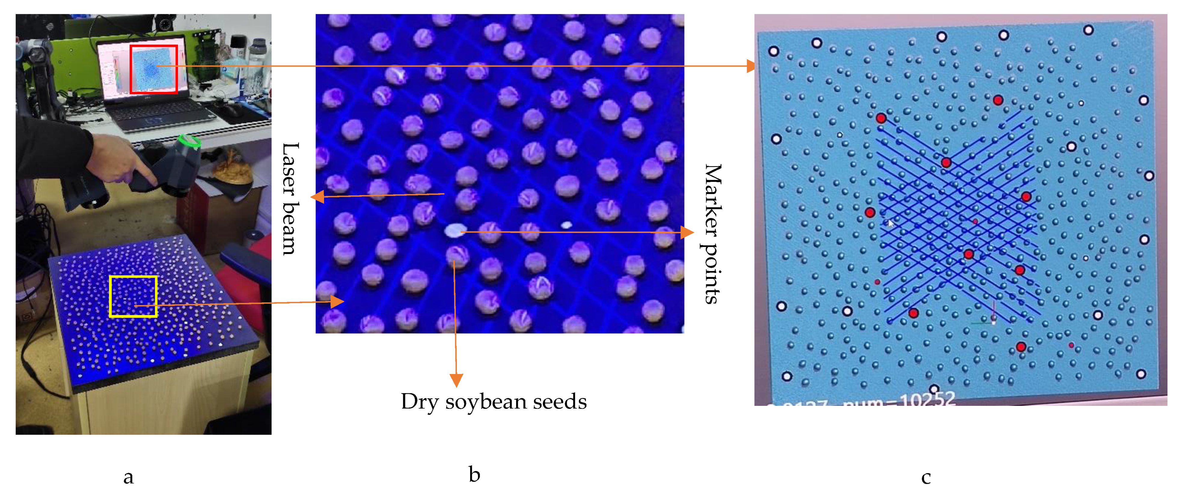
2.1. Data Acquisition and Processing Environment

Soybeans, peas, black beans, red beans, and mung beans were tested. These materials were common dry legume seeds purchased from the market and were of good quality without shriveled seeds. Each kind had uniform samples of similar size and shape. Data acquisition was performed using a handheld 3D laser scanner (RigelScan Elite made by Zhongguan Automation Technology Co., Ltd., Wuhan, China) in Wuhan, China, in September 2021. The data acquisition was conducted indoors. The RigelScan Elite scanner’s working principle is the triangulation method, which is a noncontact measurement method that uses a laser light-emitting diode. The light is focused and projected onto the target through a lens, and the reflected or diffused laser light is imaged according to a certain triangle relationship to obtain the location and spatial information of the target. The RigelScan Elite scanner has 11 pairs of cross-scanning laser beams, 1 deep-hole scanning laser beam, and 5 scanning laser beams. The basic parameters of RigelScan Elite are shown in Table 1.
Each kind of legume seed was sorted into batches, and all the seeds in a batch were scanned at once. There were no overlapped, pasted, and attached seeds. The seeds were on the table and scanned using RigelScan Elite (Figure 2a). Some reflective marker points for point cloud stitching between multiple frames were pasted on the table to assist in the acquisition of a global point cloud before scanning (Figure 2b). The scanning process was monitored from the computer in real time as it was performed. The scanner made 1,050,000 measurements per second.
Figure 2 shows the data acquisition process for a batch of soybean seeds. The obtained point cloud has no color information, and the bottom data of the seed are incomplete. The measurement accuracy is 0.010 mm.
The processing algorithm was implemented on a 2.50 GHZ desktop with 8.0 GB RAM. The code was compiled using Visual Studio 2019, Point Cloud Library (PCL) v1.8.0, and the Computational Geometry Algorithms Library (CGAL). All algorithms were integrated.

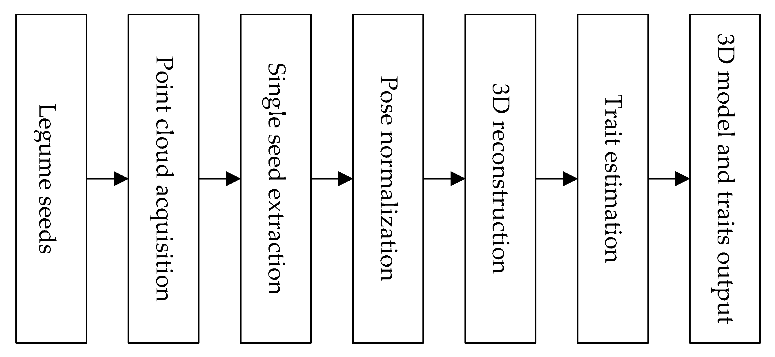
2.2. Automatic Measurement of Legume Seed Traits

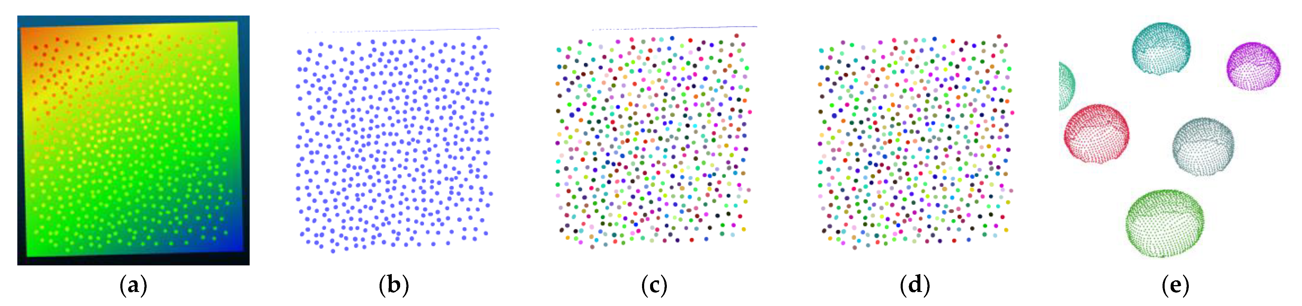
2.2.1. Single-Seed Extraction

As shown in Figure 3a, the scanned point cloud includes points from the table that should be removed. To remove these table points, the RANSAC [37] plane detection method is adopted, as shown in Figure 3b. Here, the distance threshold is 0.05 mm, and the number of neighboring points is 15. Then the Euclidean segmentation method [38] is used to extract the single seeds. Here, the distance threshold is 1 mm, and the number of neighboring points is 15. Next, a series of clusters is obtained, as shown in Figure 3c. Some clusters of the table edge points are preserved. This is because some side table points will be scanned during the data acquisition. The point clouds of the clusters of preserved table points are mainly linear or planar. Then the dimensional features [39] are used to remove these preserved table points. Performing PCA [40] on each cluster, the eigenvalues of the three principal component dimensions, λ1, λ2, and λ3 (λ1 > λ2 > λ3), can be obtained. Then the dimensions of each point cloud are calculated as follows:
a 1 D = λ 1 λ 2 λ 1 , a 2 D = λ 2 λ 3 λ 1 ,   and   a 3 D = λ 3 λ 1 ,
where a1D is a one-dimensional linear feature, a2D is a 2D planar feature, a3D is a 3D scattered point feature, and a1D + a2D + a3D = 1. Using these dimensional features of a point cloud, we can classify the point clouds as linear, planar, or 3D. A point cloud is linear when a1D is the largest and λ1 >> λ2, λ3. A point cloud is planar when a2D is the largest and λ1, λ2 >> λ3. A point cloud is 3D when a3D is the largest and λ1 ≈ λ2 ≈ λ3. This classification of the points using dimensional features allows us to remove the table points (Figure 3d).

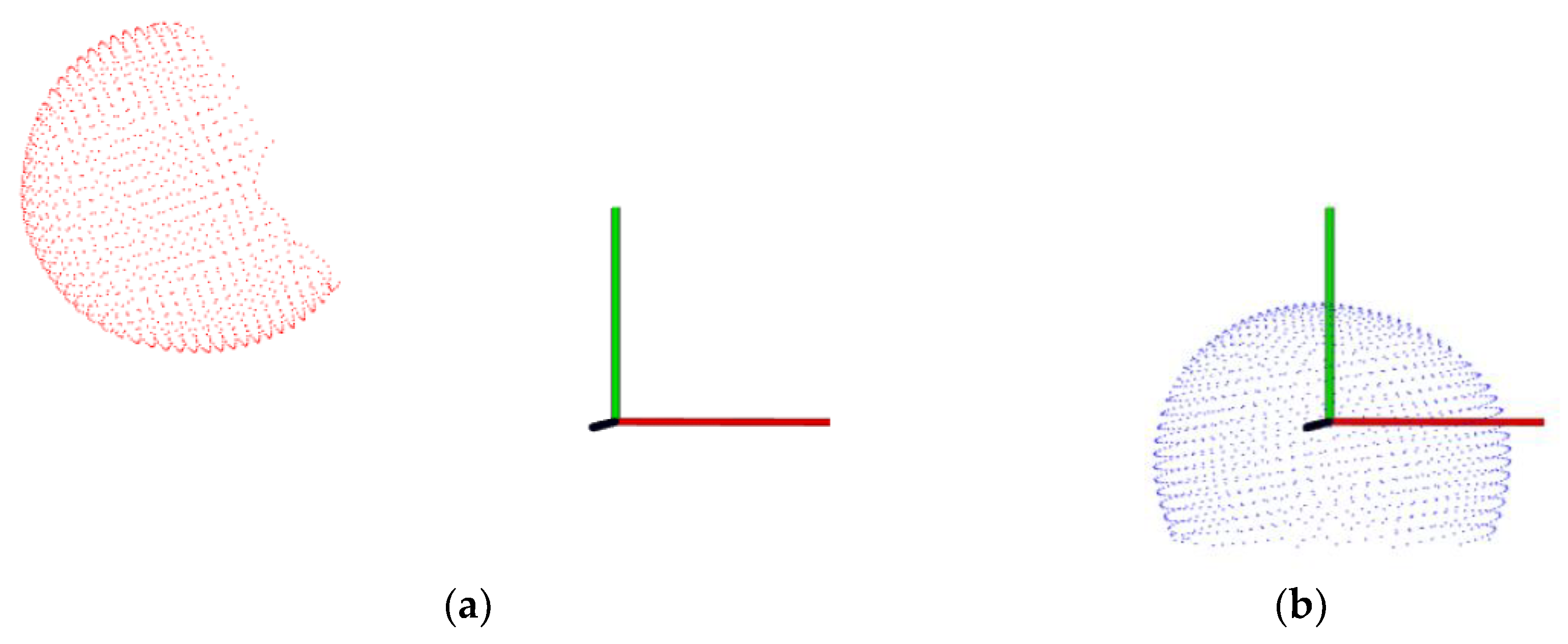
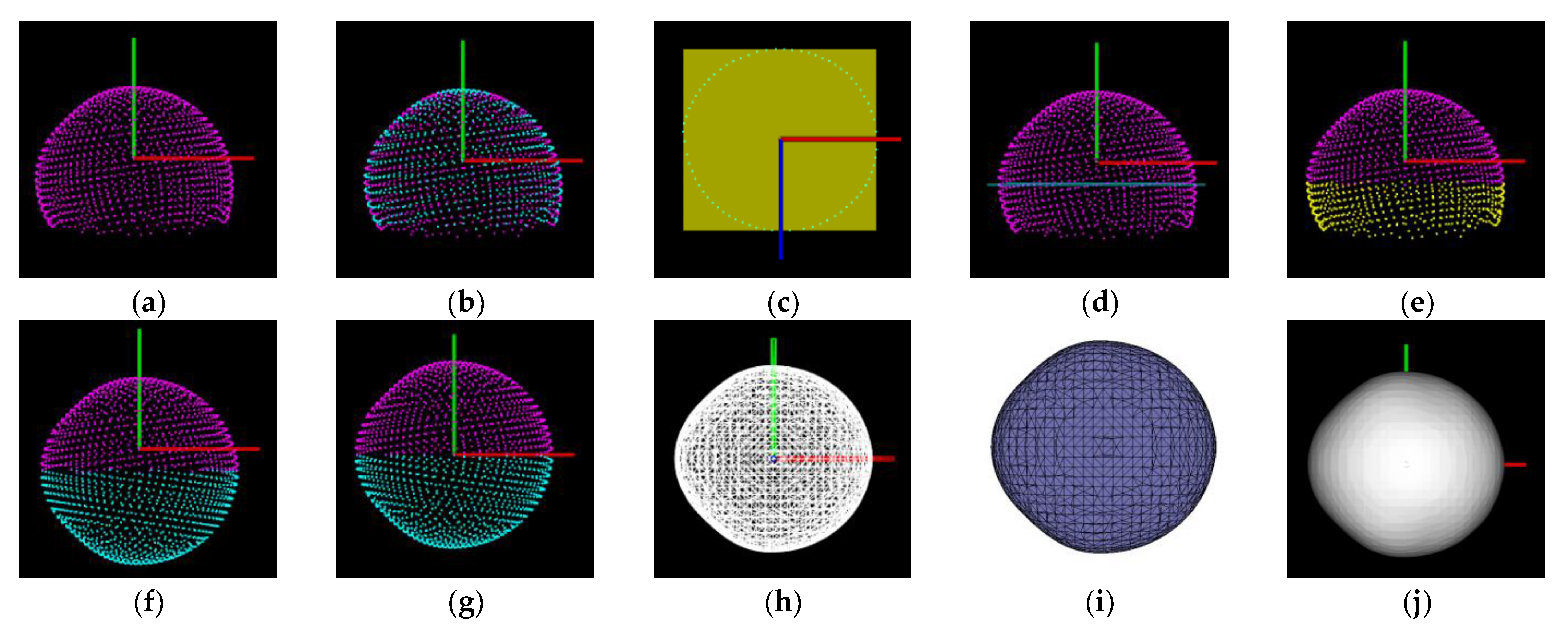
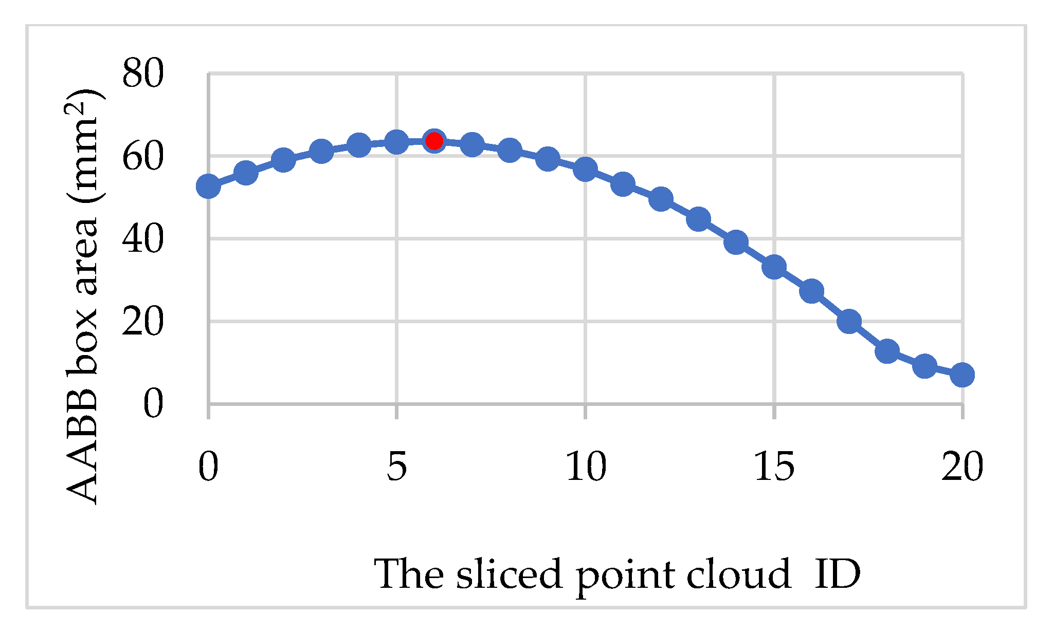
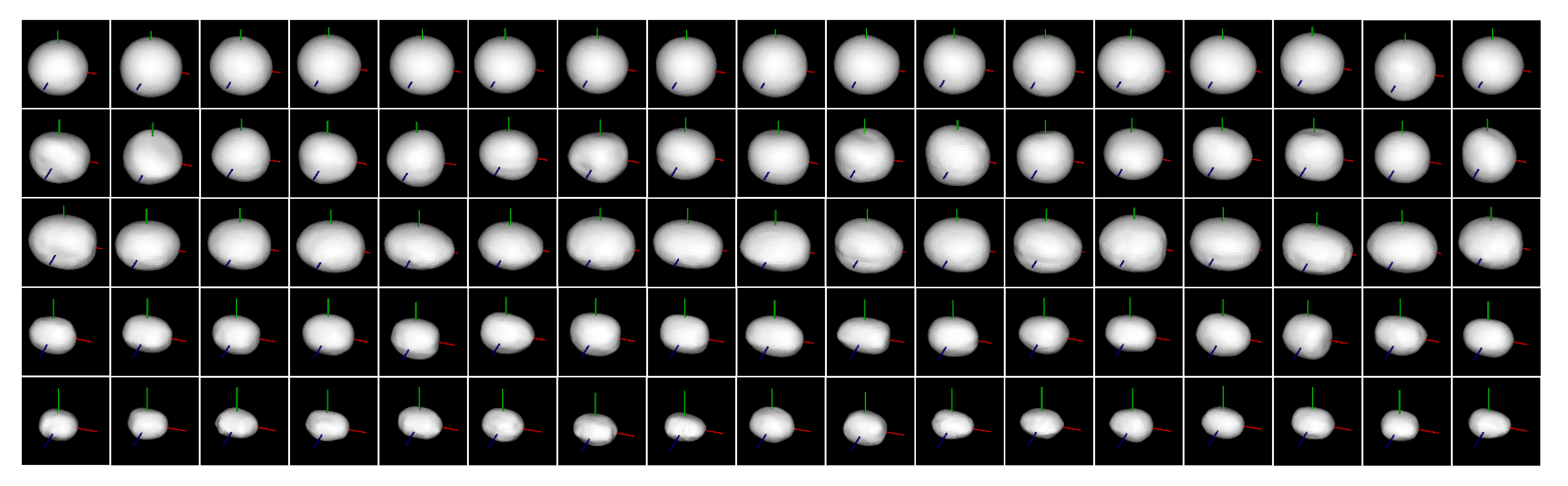
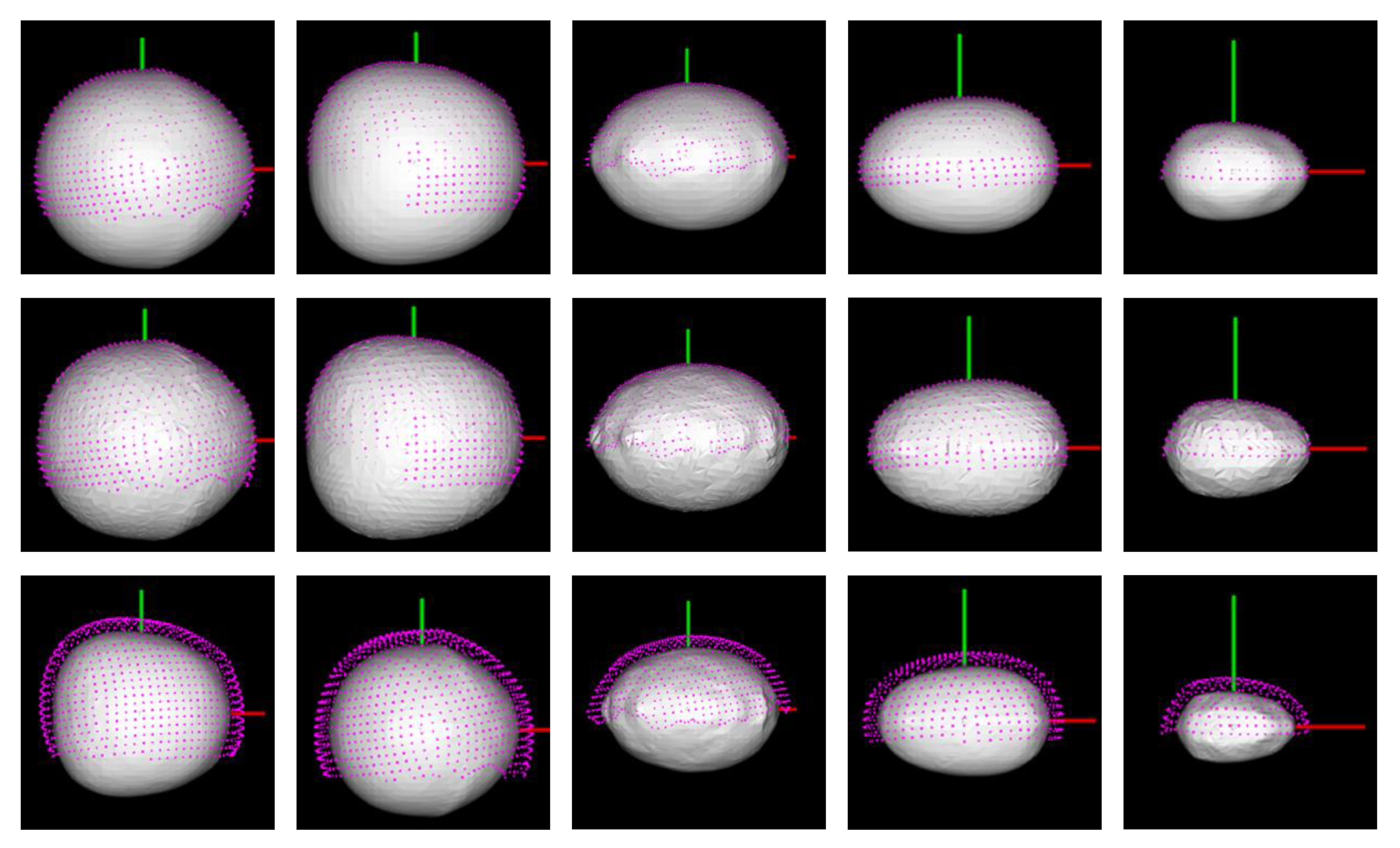
2.2.2. Pose Normalization

Normalizing the measurement pose of the individual seeds simplifies the calculation of the seeds’ traits. Here, PCA is used to perform a coordinate rotation, and the normal vector of the table is used to rectify the Y-axis direction. Performing PCA processing on the table point cloud and seed point cloud, the eigenvectors of the table point cloud (eg1, eg2, and eg3) and the eigenvectors of the seed point cloud (ev1, ev2, and ev3) are obtained. Then the coordinate rotation matrix R = [r1, r2, r3] can be calculated, where r1 = ev1 × eg2 × eg2, r2 = eg3 and r3 = ev1 × eg2.
The single-seed measurement poses in the world coordinate system are normalized after the coordinate rotation. The geometric center of the scanned point cloud of the seed is where the origin of the world coordinate system is. The table plane is horizontal to the X-axis direction and perpendicular to the Y-axis direction of the world coordinate system. The length, width, and thickness of the seed are, respectively, in the X-, Z-, and Y-axis directions of the world coordinate system, as shown in Figure 4.

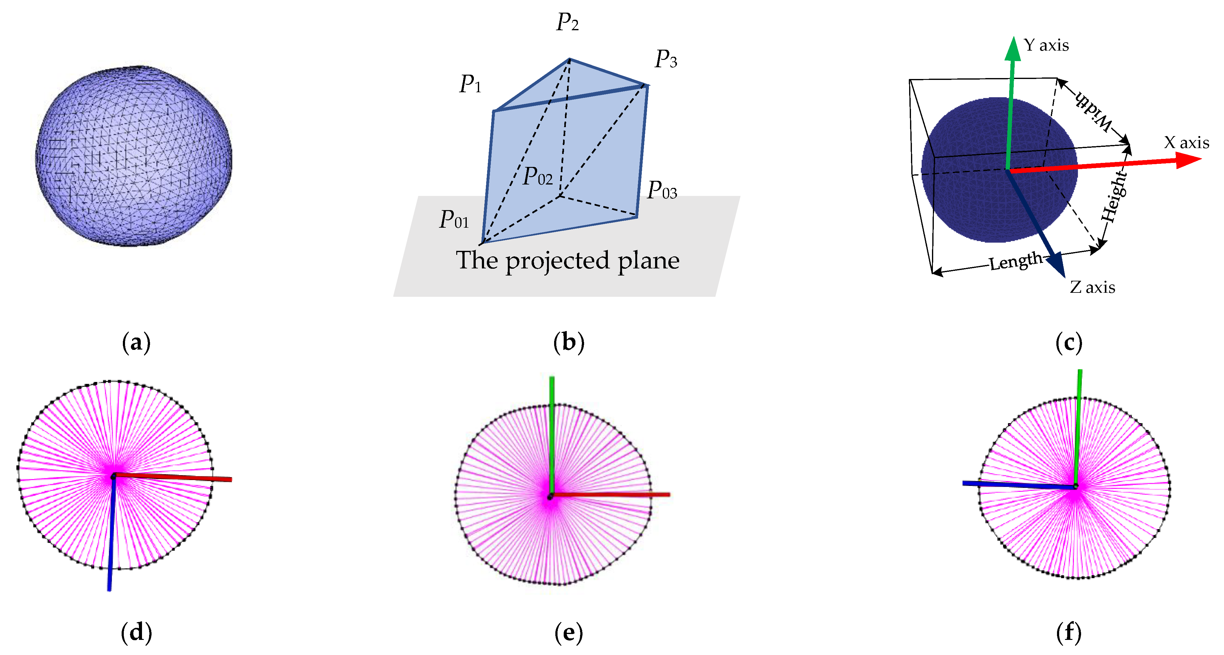
2.2.3. 3D Reconstruction

The most important thing to achieve high-throughput legume seed phenotyping based on 3D models is to obtain an accurate 3D model of the individual seeds. Since the legume seeds are placed on the table with the side of the seed facing the table, the bottom part of the seed cannot be scanned. The challenge is to obtain a complete 3D model, including the bottom part, from the incomplete scanned point cloud. Legume seeds are rigid. The shape of legume seeds, such as soybeans, peas, black beans, red beans, and mung beans, are approximately spherical or ellipsoidal [34,35,41], meaning they are almost symmetrical. Therefore, this paper exploits the geometric symmetry characteristics of legume seeds to reconstruct the 3D model based on the scanned incomplete point cloud.
The first step in 3D reconstruction is to detect the symmetry plane. The symmetry plane of the seed is often seen as the maximum principal component profile of the seed corresponding to its geometric shape. Let the single-seed point cloud be denoted PC, as shown in Figure 5a. A series of sliced point clouds, D1, D2, …, D20, are obtained by cutting PC into 20 pieces along the Y-axis, as shown in Figure 5b. Here, PC = {D1, D2, …, D20}. Then each point cloud (Di) in PC is detected by the axis-aligned bounding box (AABB box) [42], as shown in Figure 5c. The length (l) and width (w) of the box are obtained and used to compute the box area a = lw. A series of cross-sectional AABB box area values, a1, a2, …, a20, can be obtained, as shown in Figure 6. Then the position of the point cloud with the maximum AABB box area is the position of the symmetry plane. As shown in Figure 5d, the blue plane parallel to the XOZ plane is the symmetry plane.
It is now possible to use this detected symmetry plane to reconstruct a complete seed point cloud based on the incomplete scan point cloud. Suppose PC = {PC1, PC2}, where PC1 is the point cloud with the values of y greater than or equal to the symmetry plane (the magenta point cloud in Figure 5e) and PC2 is the point cloud with the values of y smaller than the symmetry plane (the yellow point cloud in Figure 5e). The mirror point cloud of PC1 based on the symmetry plane is PM (the blue point cloud in Figure 5f). Then the 3D reconstructed seed point cloud is PR = {PC1, PM}. It is worth noting that the center of the scanned point cloud and the real geometric center of the seed do not overlap due to the lack of seed bottom data during scanning. Therefore, the reconstructed point cloud is centered (Figure 5g) so that the geometric center of the seed overlaps with the origin of the coordinate system. Here, the recentered point cloud is denoted as PR’.
Surface reconstruction is necessary to measure the volume and surface area. Here, the Poisson surface reconstruction method [43] is adopted. Poisson surface reconstruction is based on the Poisson equation, which is an implicit surface reconstruction and can be calculated by:
f = 2 φ x 2 + 2 φ y 2 + 2 φ z 2 ,
where x, y, and z are the coordinate values of the points, and φ is a real-valued function that is twice differentiable in x, y, and z. Poisson surface reconstruction has the advantages of both global fitting and local fitting. Figure 5h–j shows the wireframe, triangle mesh, and surface visualization of the soybean seed’s 3D model constructed with the Poisson surface reconstruction method.

2.2.4. Trait Estimation

Morphological traits, scale factors, and shape factors are often used to describe seed size and shape. According to the related research [44,45,46,47], 11 morphological traits, 11 scale factors, and 12 shape factors are measured in this paper. These are listed in Table 2 and Table 3.
As shown in Figure 7a, the 3D seed model is triangular meshed. The seed volume (V) can be regarded as the volume of a closed space enclosed by this triangular mesh, which is the sum of the projected volumes of all the triangular patches.
V = i = 1 n ( 1 ) M V ( Δ i ) ,
where n is the number of triangles on the surface mesh, M is the direction of the triangle normal vector, and Vi) is the projected volume of the i-th triangle. The projected volume of a triangle can be seen as a convex pentahedron. Supposing a projection plane that does not intersect with all triangles in the mesh model, the projected volume is the volume of the convex pentahedron enclosed by the triangles and the projection plane. As shown in Figure 7b, a convex pentahedron, P1P2P3P01P02P03, can be divided into three tetrahedrons, and the volume of the convex pentahedron is:
V ( Δ i ) = V ( P 01 P 1 P 3 P 2 + P 01 P 2 P 3 P 03 )       , + P 01 P 2 P 03 P 02
where P1, P2, and P3 are the three vertices of the i-th triangle, and P01, P02, and P03 are the projection vertices of P1, P2, and P3 on the projection plane. If (x1, y1, z1), (x2, y2, z2), (x3, y3, z3), and (x4, y4, z4) are four vertices of a tetrahedron, the volume of the tetrahedron can be calculated by:
V ( ( x 1 , y 1 , z 1 ) , ( x 2 , y 2 , z 2 ) , ( x 3 , y 3 , z 3 ) , ( x 4 , y 4 , z 4 ) ) = 1 6 x 2 x 1 x 3 x 1 x 4 x 1 y 2 y 1 y 3 y 1 y 4 y 1 z 2 z 1 z 3 z 1 z 4 z 1 .
As shown in Figure 5a, the surface area (S) can be regarded as the total surface area of the triangular mesh.
S = i = 1 k s i ,
where n is the number of triangles on the surface mesh and si is the area of the i-th triangle.
The length (L), width (W), and thickness (H) are computed using the AABB box algorithm. As shown in Figure 7c, L, W, and H are the length, width, and height of the AABB box.
The perimeter (C) and cross-section area (A) of the three principal component profiles (horizontal (XOZ), transverse profiles (XOY), and longitudinal profiles (YOZ)) are as shown in Figure 7d–f. C is the sum of all the edges. A is the sum of the area of the triangle formed by all the edge points and the center point. C and A can be calculated as follows:
C = i = 1 m d ( i ) ,
A = i = 1 m a ( i ) ,
where m is the number of edges, d(i) is the length of the i-th edge, and a(i) is the area of the i-th triangle.
The scale factors and shape factors are calculated based on the morphological traits, as listed in Table 3.

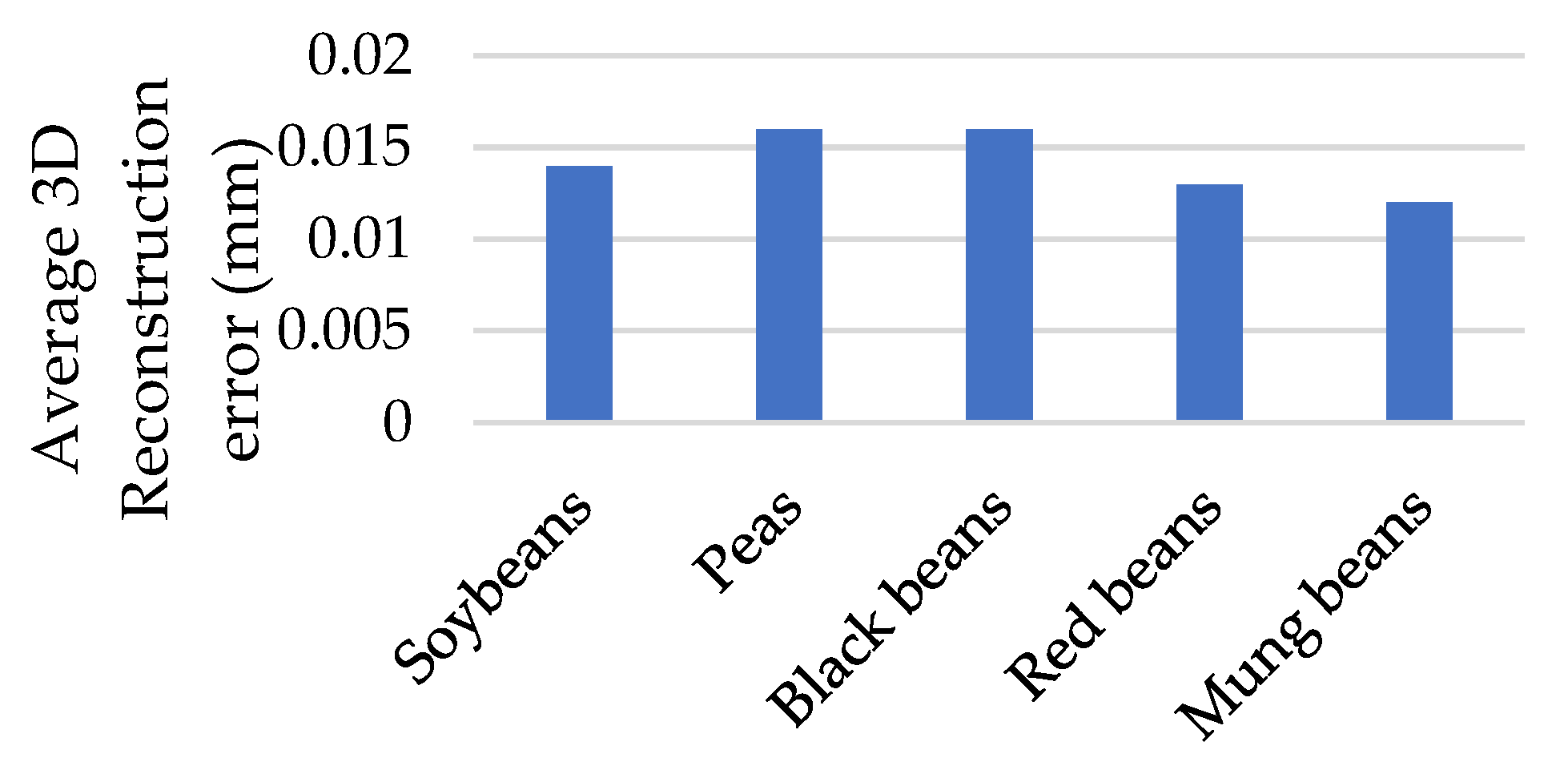
2.3. Accuracy Analysis

Data scanning, segmentation, 3D reconstruction, surface reconstruction, and trait calculation will affect the measurement accuracy.
The scanning accuracy (R_scan) and segmentation accuracy (R_seg) are calculated as follows:
R _ s c a n = N 2 N 1 × 100 %   and   R _ s e g = N 3 N 2 × 100 % ,
where N1, N2, and N3 are the numbers of total seeds, scanned seeds, and automatically extracted seeds, respectively.
Since the shape of the seed is not perfectly symmetrical, there will be a certain error between the reconstructed point cloud and the true point cloud. The error is defined as follows:
E r = 1 n i = 1 n d c l o s e t ( P i , P m j ) ,
where n is the number of the true point cloud, and dclosest (Pi, Pmj) is the distance between the true point Pi and the closest reconstructed point Pmj. The value of dclosest (Pi, Pmj) can reflect the deviation between the true point cloud and the reconstructed point cloud. If the point cloud is perfectly symmetrical, then Pi and Pmj are completely coincident, and dclosest (Pi, Pmj) = 0.
The mean absolute error (MAE), mean relative error (MRE), root mean square error (RMSE), and correlation coefficient (R) between the measured values and the true values are used to verify the accuracy of measurement traits.
M A E = 1 n i = 1 n | x a i x m i | ,
M R E = 1 n i = 1 n | x a i x m i | x m i × 100 % ,
R M S E = 1 n i = 1 n ( x a i x m i ) 2 ,
R ( x a i , x m i ) = C ov ( x a i , x m i ) V a r [ x a i ] V a r [ x m i ] ,

3. Results

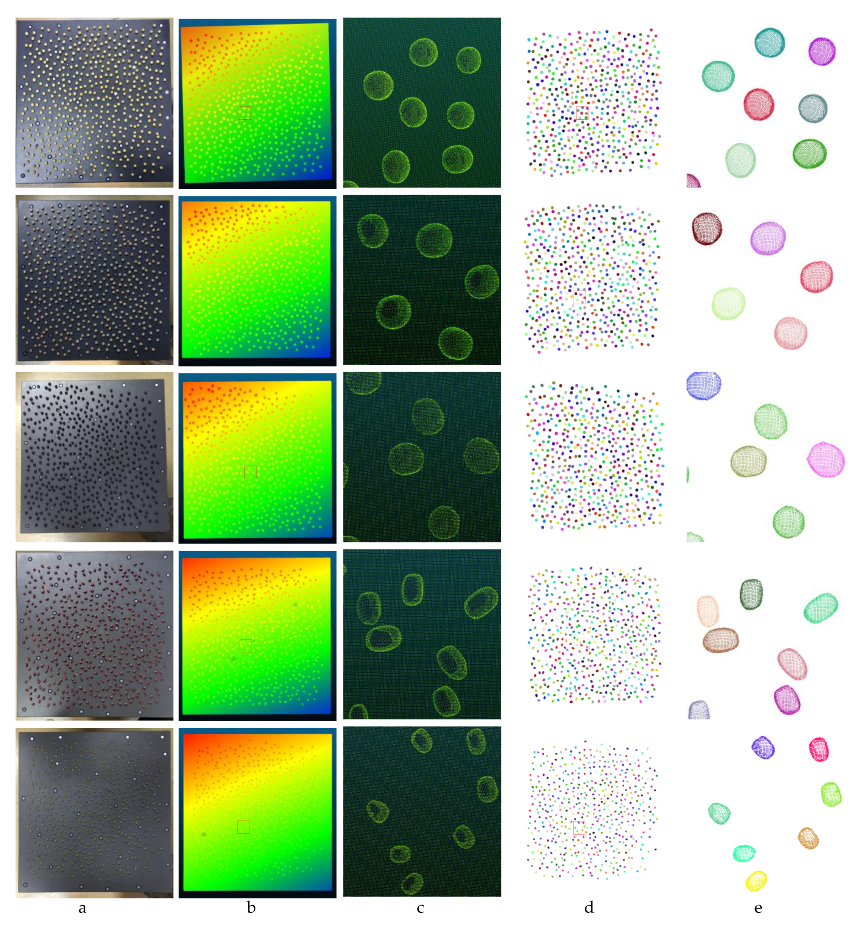
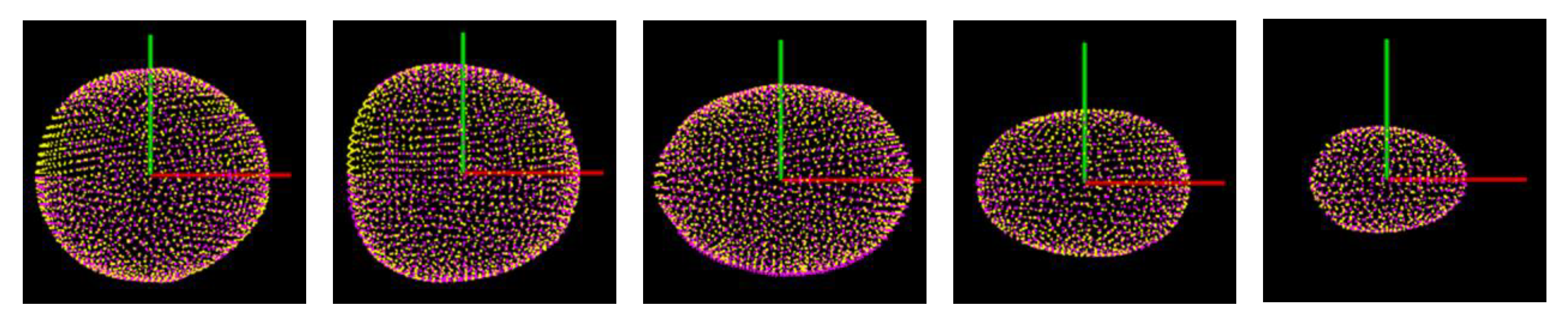
3.1. Visualization of Scanning and Segmentation Results

Figure 8 shows the scanning and segmentation results of soybeans, peas, black beans, red beans, and mung beans. As shown in Figure 8a, each kind is scanned at once in a batch. The point clouds of most legume seeds are successfully obtained, and the acquired point cloud has no seed bottom data, as shown in Figure 8c. All successfully scanned point clouds are successfully segmented, as shown in Figure 8d. It should be noted that the obtained point cloud is with no color information, and the scanned results in Figure 8b,c are rendered for effective visualization because of the 0.01 mm high-density point cloud.

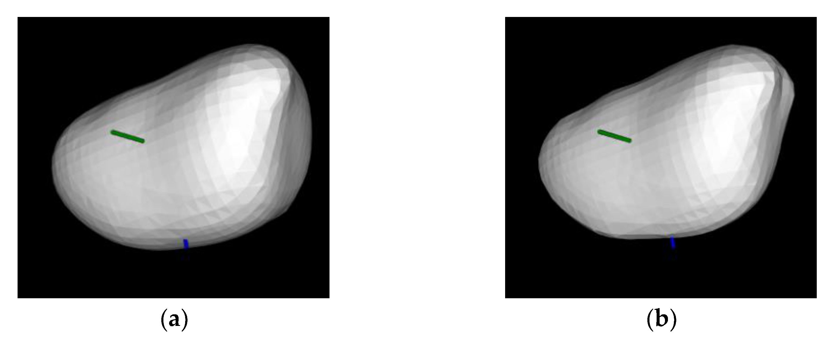
3.2. Visualization of 3D Reconstruction

Figure 9 shows parts of the 3D reconstruction results. From first to last, the rows are soybean, pea, black bean, red bean, and mung bean seeds, respectively. The surface mesh is closed and smooth. Soybean, pea, and black bean seeds have a larger size than those of red bean and mung bean. Soybeans, peas, and black beans have approximately spherical seeds, whereas red beans and mung beans have seeds that are similar to an ellipsoid. Soybean seeds are rounder than pea and black bean seeds.

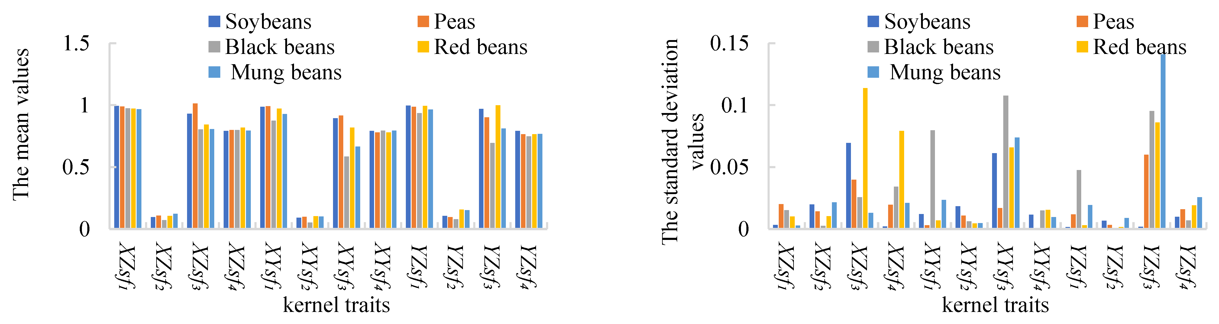
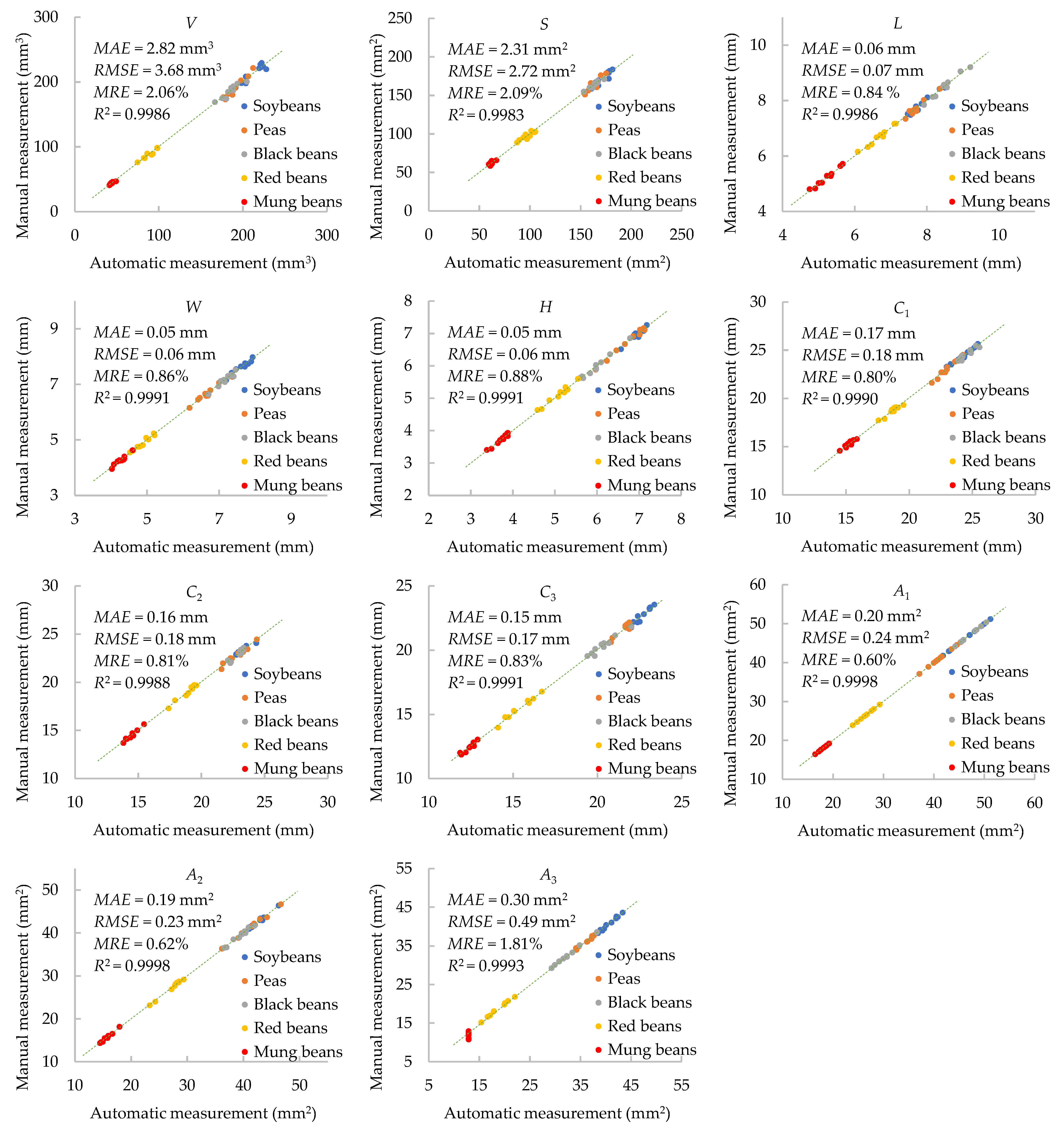
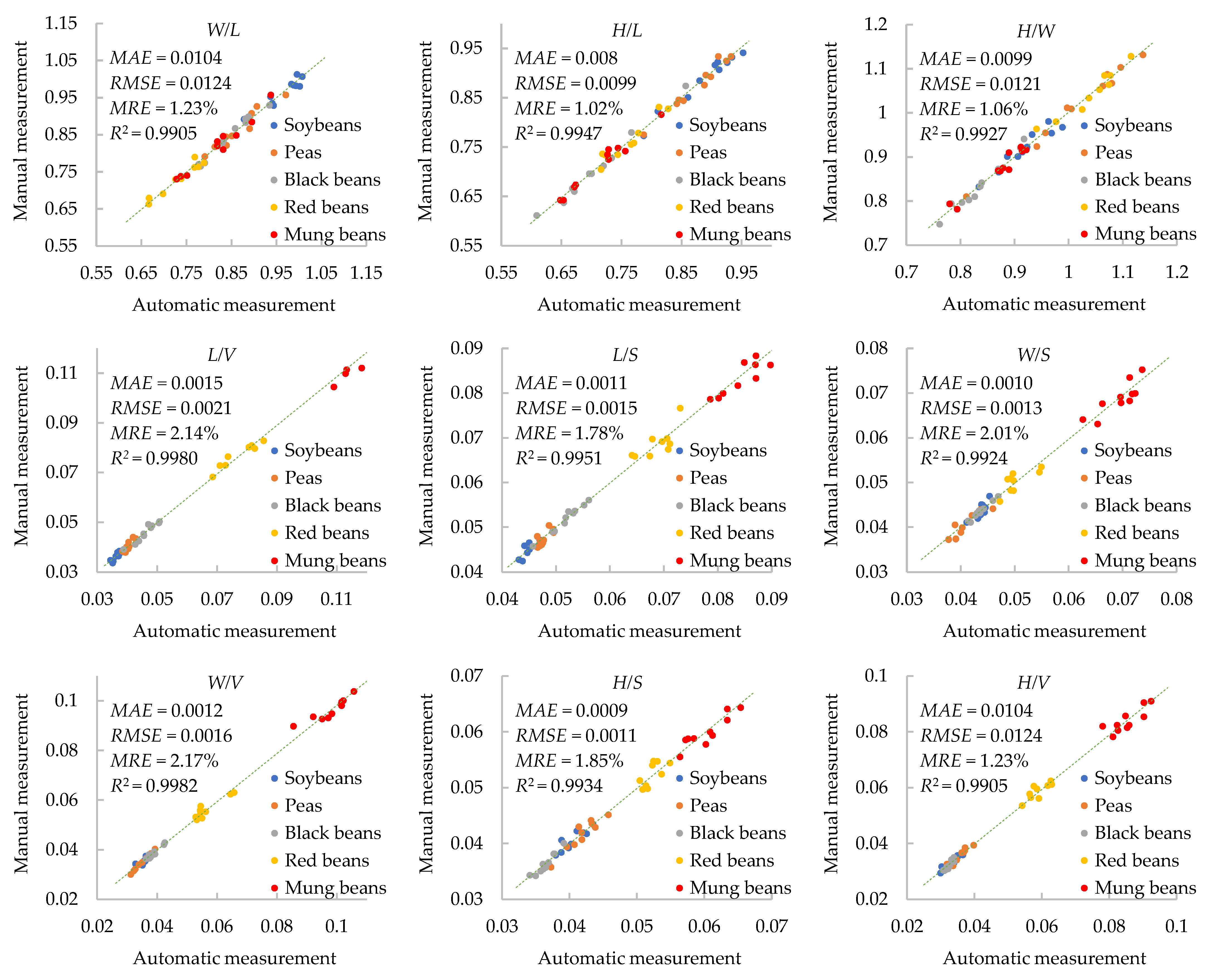
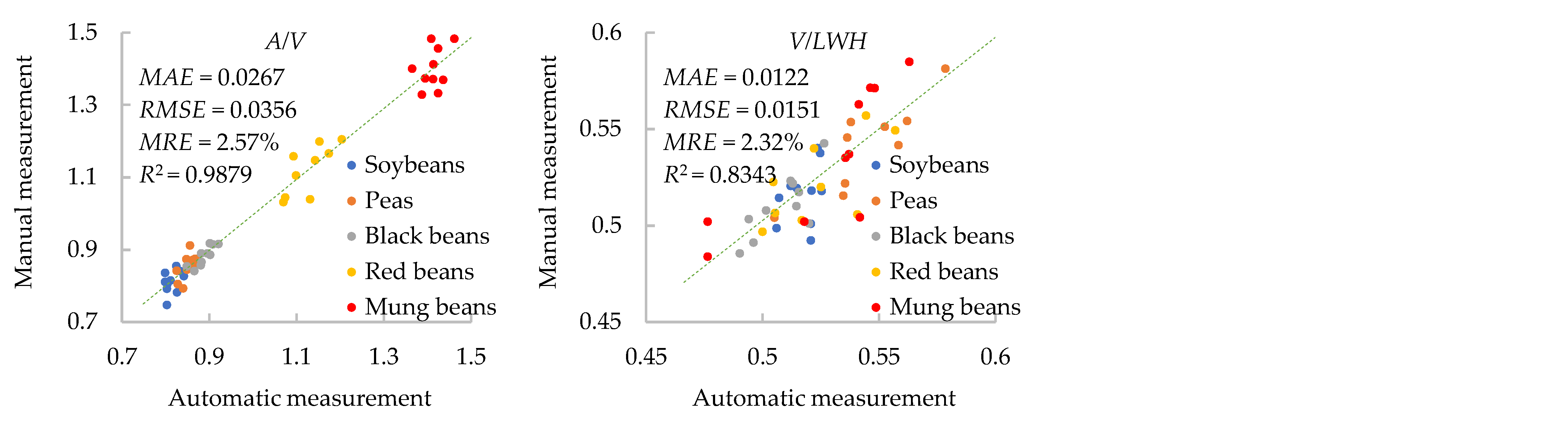
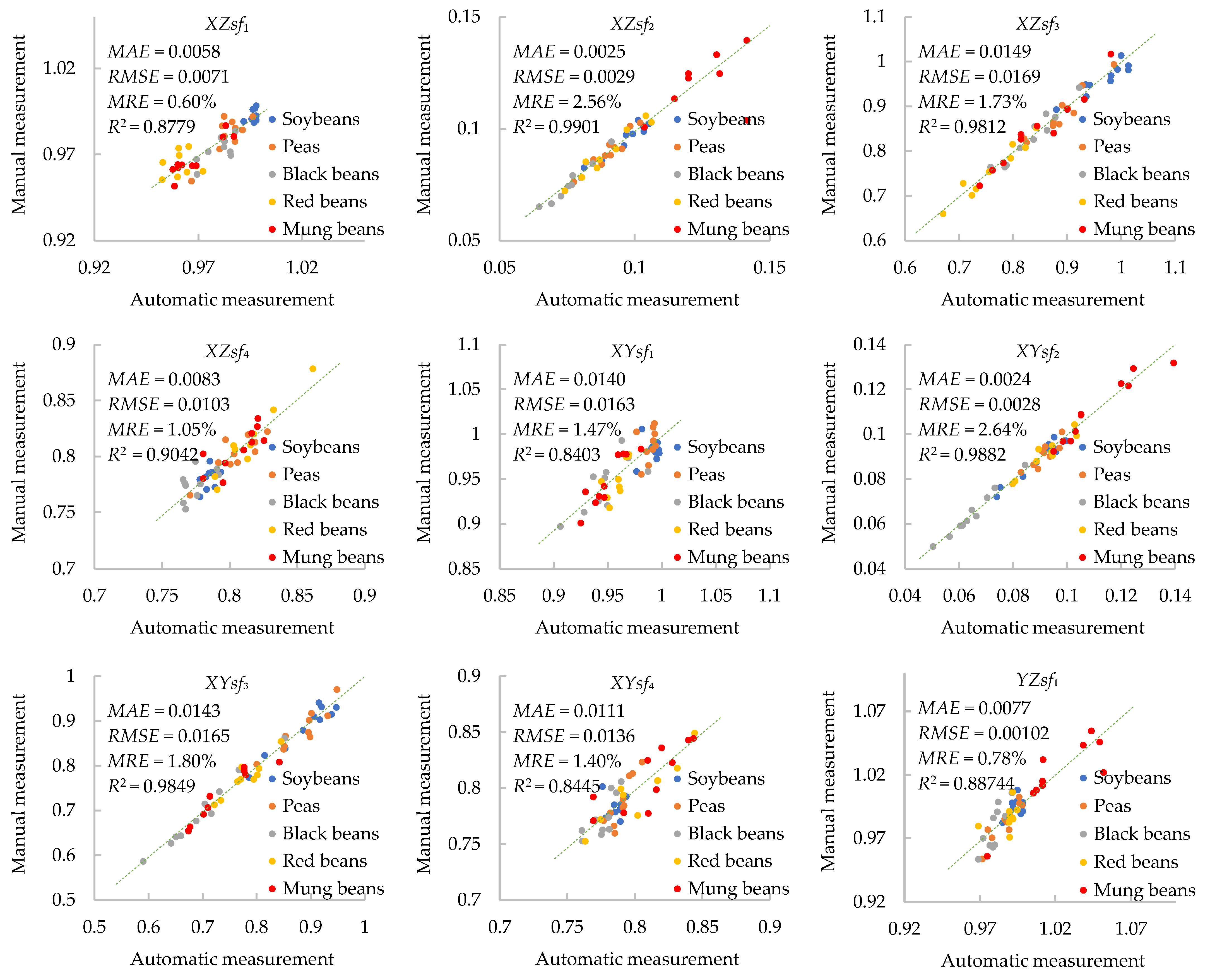
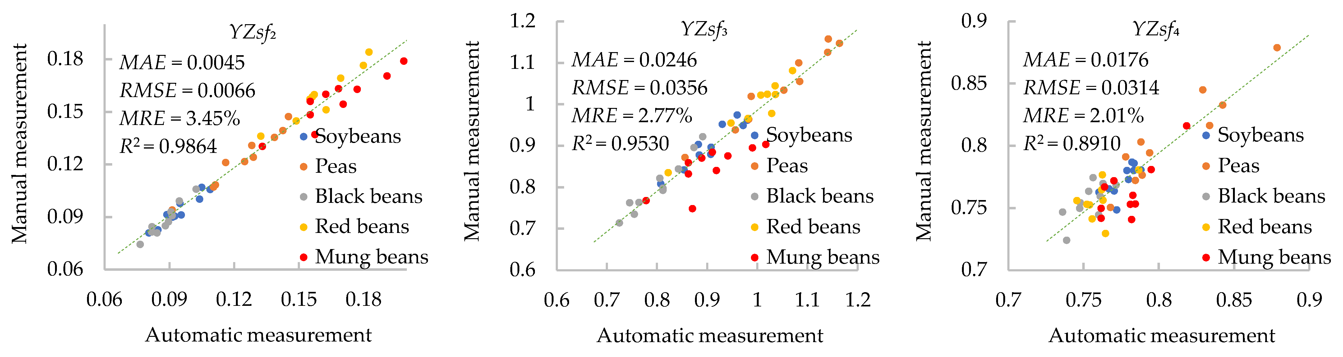
3.3. Results of Trait Estimation

The measured mean values and the corresponding standard deviation values of kernel traits of five kinds of legume seeds are shown in Figure 10. Different types of bean seeds have different values of morphological traits, scale factors, and shape factors. The scale and shape traits have a smaller deviation compared with the morphological traits.

3.4. Time Cost

Table 4 lists the computing time required for each experiment. For all the experiments, the data scanning time ranges from 220 s to 265 s. The data processing time, including segmentation and trait estimation, varies from 16.24 s to 20.43 s. Most of the time is spent on data scanning. In general, it takes 0.52 s to estimate 34 traits of one seed, including the data acquisition and trait calculation.

4. Discussion

In this work, a high-throughput legume seed phenotyping method using a handheld 3D laser scanner is presented. All the data processing was conducted by algorithms without any manual input required. To verify the utility of the proposed method, the accuracies of the data scanning, segmentation, 3D reconstruction, surface reconstruction, and trait calculation need to be discussed.

4.1. Accuracy of Data Scanning and Segmentation

Depending on the species of the seed, the background of the image could be changed to obtain more adequate scanning data. The background in this paper is the same dark gray. The experiments show that 2488 of the 2500 samples were successfully scanned. This illustrates that the proposed data acquisition using RigelScan Elite is effective and robust.
The scanning accuracies of soybean, pea, black bean, red bean, and mung bean seeds are 100%, 100%, 99.00%, 99.40%, and 99.20%, respectively. The average scanning accuracy is 99.52%.
The scanning accuracies vary among different legume seeds. The main reasons for this variation are the differences in surface color and reflection. The seeds of soybeans and peas are light colored, and their surfaces are not very reflective. Black beans, red beans, and mung beans, however, are dark colored and have more reflective surfaces. This causes the scanning accuracy of the soybean and pea seeds to be higher than that of the black bean, red bean, and mung bean seeds. Black beans have the lowest scanning accuracy because their surface color is very close to the background, and they have the most reflection among the five kinds of legume seed studied.
The accuracy of the segmentation is 100%. This high segmentation accuracy is because there are no attached seeds during data scanning.

4.2. Accuracy of 3D Reconstruction

The validity of the reconstructed 3D model directly affects the correctness of the trait measurements. To compare the reconstructed model with real data, complete point clouds were obtained using the RigelScan Elite. To do this, a single seed was skewered on a long needle, which was then affixed to the table, and the seed was scanned in detail to get its complete point cloud. It took approximately 90 s to obtain a detailed and complete point cloud of a single seed. A total of 10 samples of each kind of legume seed were individually scanned. The reconstructed point clouds (magenta point clouds) and the artificially scanned point clouds (yellow point clouds) are presented in Figure 11. The reconstructed point cloud has a high overlap with the real scanned point cloud. The deviation can hardly be seen visually.
As shown in Figure 12, the average reconstruction error for soybeans, peas, black beans, red beans, and mung beans are 0.014, 0.016, 0.016, 0.013, and 0.012 mm, respectively. The overall average reconstruction error is 0.014 mm. It can be found that the shapes of soybean, pea, and red bean seeds have better symmetry than those of black beans and mung beans.

4.3. Comparison of Surface Reconstruction Methods

Poisson surface reconstruction, greedy triangulation [48], and marching cube surface reconstruction [49] are three classic surface reconstruction methods, and the results of each method are shown in Figure 13. The meshes built by the greedy triangulation algorithm are rough and not smooth enough. The meshes built by the marching cube surface reconstruction method do not effectively match the scanned point clouds. The meshes built by the Poisson surface reconstruction algorithm are closed and smooth and express the data from the original scanned points well.
It can be verified that the 3D mesh of a legume seed built by the Poisson surface reconstruction method is smooth and watertight. This 3D model of the legume seed is very close to the true shape of the seed.

4.4. Accuracy of Trait Estimation

From the scanned 2500 samples, 50 seeds (the same seeds as in Section 4.2) were measured manually to evaluate the algorithm performance. The ground truths of length, width, and thickness were obtained using a vernier caliper. The other traits were measured by the software Geomagic Studio based on the real 3D point cloud obtained in Section 4.2. All the ground truths were manually measured three times by three people, and the average was adopted.
The measurement accuracies of 11 morphological traits, 11 scale factors, and 12 shape factors are shown in Figure 14, Appendix A, and Appendix B. The values of MAE, RMSE, MRE, and R2 of these kernel traits are presented in detail. The average absolute measurement accuracy and root mean square error are in submillimeter, the average relative measurement accuracy is within 3%, and R2 is above 0.9983 for the 11 morphological traits. The average relative measurement accuracy is within 4%, and R2 for the 11 morphological traits is above 0.8343 for 11 scale factors and 12 shape factors. The experiments show that the measurement accuracy of the proposed method is comparable to previous work in this area [6,44,50]. Moreover, the proposed method shows the viability and effectiveness of automatic estimation and batch extraction of seeds’ geometric parameters, especially their 3D traits.

4.5. Advantages, Limitations, Improvements, and Future Work

A high-throughput legume seed phenotyping method is proposed in this paper. The handheld scanner RigelScan Elite can rapidly obtain point clouds of legume seeds in batches with an accuracy of 0.01 mm. The 3D model of a single seed can be reconstructed with an average reconstruction error of 0.014 mm. A total of 34 legume seed traits, notably the longitudinal and transverse profiles traits, can be automatically extracted in batches. The measurement accuracy is within 4% for all the morphological traits. The measurement takes an average time per seed of 0.52 s. The results demonstrate the ability of the proposed method to perform data batch processing and automatic measurement, which shows potential for real-time measurement and high-throughput phenotyping.
The extracted 34 trait indicators in this paper have prospects and research value in application in precision agriculture. The morphological traits, such as the volume, surface area, length, width, thickness, horizontal profile perimeter, transverse profile perimeter, longitudinal profile perimeter, horizontal profile cross-section area, transverse profile cross-section area, and longitudinal profile cross-section area, can directly quantitatively describe the seed size, which is important in quality evaluation, optimization breeding, and yield evaluation. The scale traits and shape factors can quantitatively describe the seed shape, which can be helpful in species identification and classification and quantitative trait loci.
It should be noted that the 3D reconstruction approach proposed in this paper is suitable for seeds with symmetrical geometrical shapes, but its use is limited for seeds with asymmetrical geometry. The proposed method will fail when the seed has no symmetrical shape. As shown in Figure 15, the 3D peanut model reconstructed by our algorithm has a big difference from the real one. Therefore, a 3D reconstruction method that is suitable for seeds with diverse geometric shapes is a potential avenue for further research.
Further work will seek a more robust 3D reconstruction method that works for various seeds. In addition, seed classification and quality evaluation based on these extracted traits will be discussed.

5. Conclusions

This paper presents a novel high-throughput legume seed phenotyping method. The objective of the proposed method is to realize automatic measurement and batch data processing in legume seed measurement. This goal has been achieved by an automatic pipeline of data acquisition and processing, including data acquisition using a handheld 3D laser scanner, RigelScan Elite, with 99.52% scanning accuracy; single-seed extraction with 100% segmentation accuracy; pose normalization; 3D reconstruction using a symmetry-based 3D reconstruction method with 0.014 mm reconstruction error; and trait estimation with average relative measurement accuracy within 4%.
Since the 3D reconstruction method proposed in this paper is symmetry based, the proposed method has limitations when measuring seeds with irregular geometrical shapes. The study can be improved if a more effective 3D reconstruction method suitable for seeds with diverse shapes is used. In addition, there are no overlapping and pasting seeds in our experiment. Further research will explore an effective segmentation method where seeds are overlapping and pasting.
The high measurement accuracy, the low time cost, and the ability to handle batch data processing and automatic measurement have shown that the proposed method has the potential for high-throughput legume seed phenotyping. It can promote automation in seed quality evaluation, optimization breeding, and a yield trait scorer, where large samples are required. We also plan to integrate the proposed method into a handheld scanner system to achieve real-time seed measurement.

Author Contributions

Conceptualization, X.H.; methodology, X.H.; validation, X.H.; formal analysis, X.H.; writing—original draft preparation, X.H.; writing—review and editing, X.H and S.Z.; visualization, X.H.; supervision, S.Z. and N.Z.; funding acquisition, S.Z. and N.Z. All authors have read and agreed to the published version of the manuscript.

Funding

This work was supported by the Natural Sciences Foundation of China (Grant No. 41671452, 41701532,42101446).

Data Availability Statement

Data and code from this research will be available upon request to the authors.

Acknowledgments

The authors sincerely thank anonymous reviewers and members of the editorial team for their comments.

Conflicts of Interest

The authors declare no conflict of interest.

Appendix A

Figure A1. Measurement accuracies of 11 scale factors.
Remotesensing 14 00431 g0a1aRemotesensing 14 00431 g0a1b

Appendix B

Figure A2. Measurement accuracies of 12 shape factors.
Remotesensing 14 00431 g0a2aRemotesensing 14 00431 g0a2b

References

  1. Zhu, X.; Zhao, Z. Measurement and analysis of fluorescent whitening agent content in soybean milk based on image techniques. Measurement 2016, 94, 213–220. [Google Scholar] [CrossRef]
  2. Sosa, E.F.; Thompson, C.; Chaves, M.G.; Acevedo, B.A.; Avanza, M. V Legume seeds treated by high hydrostatic pressure: Effect on functional properties of flours. Food Bioprocess Technol. 2020, 13, 323–340. [Google Scholar] [CrossRef]
  3. Mahajan, S.; Das, A.; Sardana, H.K. Image acquisition techniques for assessment of legume quality. Trends Food Sci. Technol. 2015, 42, 116–133. [Google Scholar] [CrossRef]
  4. Mittal, S.; Dutta, M.K.; Issac, A. Non-destructive image processing based system for assessment of rice quality and defects for classification according to inferred commercial value. Measurement 2019, 148, 106969–106977. [Google Scholar] [CrossRef]
  5. Afzal, M.; Alghamdi, S.S.; Migdadi, H.H.; Khan, M.A.; Mirza, S.B.; El-Harty, E. Legume genomics and transcriptomics: From classic breeding to modern technologies. Saudi J. Biol. Sci. 2020, 27, 543–555. [Google Scholar] [CrossRef]
  6. Warman, C.; Sullivan, C.M.; Preece, J.; Buchanan, M.E.; Vejlupkova, Z.; Jaiswal, P.; Fowler, J.E. A cost-effective maize ear phenotyping platform enables rapid categorization and quantification of kernels. Plant J. 2021, 106, 566–579. [Google Scholar] [CrossRef] [PubMed]
  7. Cao, X.; Yan, H.; Huang, Z.; Ai, S.; Xu, Y.; Fu, R.; Zou, X. A multi-objective particle swarm optimization for trajectory planning of fruit picking manipulator. Agronomy 2021, 11, 2286. [Google Scholar] [CrossRef]
  8. Wu, F.; Duan, J.; Chen, S.; Ye, Y.; Ai, P.; Yang, Z. Multi-target recognition of bananas and automatic positioning for the inflorescence axis cutting point. Front. Plant Sci. 2021, 12, 1–15. [Google Scholar] [CrossRef]
  9. Chen, M.; Tang, Y.; Zou, X.; Huang, Z.; Zhou, H.; Chen, S. 3D global mapping of large-scale unstructured orchard integrating eye-in-hand stereo vision and SLAM. Comput. Electron. Agric. 2021, 187, 106237. [Google Scholar] [CrossRef]
  10. Gu, S.; Liao, Q.; Gao, S.; Kang, S.; Du, T.; Ding, R. Crop water stress index as a proxy of phenotyping maize performance under combined water and salt stress. Remote Sens. 2021, 13, 4710. [Google Scholar] [CrossRef]
  11. Margapuri, V.; Courtney, C.; Neilsen, M. Image processing for high-throughput phenotyping of seeds. Epic Ser. Comput. 2021, 75, 69–79. [Google Scholar] [CrossRef]
  12. Herzig, P.; Borrmann, P.; Knauer, U.; Klück, H.-C.; Kilias, D.; Seiffert, U.; Pillen, K.; Maurer, A. Evaluation of RGB and multispectral unmanned aerial vehicle (UAV) imagery for high-throughput phenotyping and yield prediction in barley breeding. Remote Sens. 2021, 13, 2670. [Google Scholar] [CrossRef]
  13. Mussadiq, Z.; Laszlo, B.; Helyes, L.; Gyuricza, C. Evaluation and comparison of open source program solutions for automatic seed counting on digital images. Comput. Electron. Agric. 2015, 117, 194–199. [Google Scholar] [CrossRef]
  14. Fıratlıgil-Durmuş, E.; Šárka, E.; Bubník, Z.; Schejbal, M.; Kadlec, P. Size properties of legume seeds of different varieties using image analysis. J. Food Eng. 2010, 99, 445–451. [Google Scholar] [CrossRef]
  15. Singh, S.K.; Vidyarthi, S.K.; Tiwari, R. Machine learnt image processing to predict weight and size of rice kernels. J. Food Eng. 2020, 274, 109828–109838. [Google Scholar] [CrossRef]
  16. Igathinathane, C.; Pordesimo, L.O.; Columbus, E.P.; Batchelor, W.D.; Methuku, S.R. Shape identification and particles size distribution from basic shape parameters using ImageJ. Comput. Electron. Agric. 2008, 63, 168–182. [Google Scholar] [CrossRef]
  17. Carpenter, A.E.; Jones, T.R.; Lamprecht, M.R.; Clarke, C.; Kang, I.H.; Friman, O.; Guertin, D.A.; Chang, J.H.; Lindquist, R.A.; Moffat, J. CellProfiler: Image analysis software for identifying and quantifying cell phenotypes. Genome Biol. 2006, 7, 1–11. [Google Scholar] [CrossRef] [PubMed] [Green Version]
  18. Dong, R.; Jahufer, M.Z.Z.; Dong, D.K.; Wang, Y.R.; Liu, Z.P. Characterisation of the morphological variation for seed traits among 537 germplasm accessions of common vetch (Vicia sativa L.) using digital image analysis. N. Z. J. Agric. Res. 2016, 59, 422–435. [Google Scholar] [CrossRef]
  19. Tanabata, T.; Shibaya, T.; Hori, K.; Ebana, K.; Yano, M. SmartGrain: High-throughput phenotyping software for measuring seed shape through image analysis. Plant Physiol. 2012, 160, 1871–1880. [Google Scholar] [CrossRef] [Green Version]
  20. Faroq, A.-T.; Adam, H.; Dos Anjos, A.; Lorieux, M.; Larmande, P.; Ghesquière, A.; Jouannic, S.; Shahbazkia, H.R. P-TRAP: A panicle trait phenotyping tool. BMC Plant Biol. 2013, 13, 1–14. [Google Scholar] [CrossRef] [Green Version]
  21. Chen, M.; Tang, Y.; Zou, X.; Huang, K.; Huang, Z.; Zhou, H.; Wang, C.; Lian, G. Three-dimensional perception of orchard banana central stock enhanced by adaptive multi-vision technology. Comput. Electron. Agric. 2020, 174, 105508. [Google Scholar] [CrossRef]
  22. Lin, G.; Tang, Y.; Zou, X.; Xiong, J.; Fang, Y. Color-, depth- and shape-based 3D fruit detection. Precis. Agric. 2020, 21, 1–17. [Google Scholar] [CrossRef]
  23. Yang, S.; Zheng, L.; Gao, W.; Wang, B.; Hao, X.; Mi, J.; Wang, M. An efficient processing approach for colored point cloud-based high-throughput seedling phenotyping. Remote Sens. 2020, 12, 1540. [Google Scholar] [CrossRef]
  24. Miao, T.; Zhu, C.; Xu, T.; Yang, T.; Li, N.; Zhou, Y.; Deng, H. Automatic stem-leaf segmentation of maize shoots using three-dimensional point cloud. Comput. Electron. Agric. 2021, 187, 106310. [Google Scholar] [CrossRef]
  25. Zhang, Z.; Ma, X.; Guan, H.; Zhu, K.; Feng, J.; Yu, S. A method for calculating the leaf inclination of soybean canopy based on 3D point clouds. Int. J. Remote Sens. 2021, 42, 5721–5742. [Google Scholar] [CrossRef]
  26. De Souza, C.H.W.; Lamparelli, R.A.C.; Rocha, J.V.; Magalhães, P.S.G. Height estimation of sugarcane using an unmanned aerial system (UAS) based on structure from motion (SfM) point clouds. Int. J. Remote Sens. 2017, 38, 2218–2230. [Google Scholar] [CrossRef]
  27. Li, M.; Shamshiri, R.R.; Schirrmann, M.; Weltzien, C. Impact of camera viewing angle for estimating leaf parameters of wheat plants from 3D point clouds. Agriculture 2021, 11, 563. [Google Scholar] [CrossRef]
  28. Harwin, S.; Lucieer, A.; Osborn, J. The impact of the calibration method on the accuracy of point clouds derived using unmanned aerial vehicle multi-view stereopsis. Remote Sens. 2015, 7, 1933. [Google Scholar] [CrossRef] [Green Version]
  29. Wen, W.; Guo, X.; Lu, X.; Wang, Y.; Yu, Z. Multi-scale 3D data acquisition of maize. In International Conference on Computer and Computing Technologies in Agriculture; Springer: Berlin/Heidelberg, Germany, 2017; pp. 108–115. [Google Scholar]
  30. Roussel, J.; Geiger, F.; Fischbach, A.; Jahnke, S.; Scharr, H. 3D surface reconstruction of plant seeds by volume carving: Performance and accuracies. Front. Plant Sci. 2016, 7, 745–758. [Google Scholar] [CrossRef] [Green Version]
  31. Li, H.; Qian, Y.; Cao, P.; Yin, W.; Dai, F.; Hu, F.; Yan, Z. Calculation method of surface shape feature of rice seed based on point cloud. Comput. Electron. Agric. 2017, 142, 416–423. [Google Scholar] [CrossRef]
  32. Su, Y.; Xiao, L.-T. 3D visualization and volume-based quantification of rice chalkiness in Vivo by using high resolution Micro-CT. Rice 2020, 13, 1–12. [Google Scholar] [CrossRef]
  33. Cervantes, E.; Martín Gómez, J.J. Seed shape description and quantification by comparison with geometric models. Horticulturae 2019, 5, 60. [Google Scholar] [CrossRef] [Green Version]
  34. Xu, T.; Yu, J.; Yu, Y.; Wang, Y. A modelling and verification approach for soybean seed particles using the discrete element method. Adv. Powder Technol. 2018, 29, 3274–3290. [Google Scholar] [CrossRef]
  35. Yang, S.; Zheng, L.; He, P.; Wu, T.; Sun, S.; Wang, M. High-throughput soybean seeds phenotyping with convolutional neural networks and transfer learning. Plant Methods 2021, 17, 1–17. [Google Scholar] [CrossRef] [PubMed]
  36. Huang, X.; Zheng, S.; Gui, L.; Zhao, L.; Ma, H. Automatic extraction of high-throughput phenotypic information of grain based on point cloud. Trans. Chin. Soc. Agric. Mach 2018, 49, 257–264. [Google Scholar]
  37. Schnabel, R.; Wahl, R.; Klein, R. Efficient RANSAC for point-cloud shape detection. In Computer Graphics Forum; Wiley Online Library: Hoboken, NJ, USA, 2007; Volume 26, pp. 214–226. [Google Scholar]
  38. Nüchter, A.; Rusu, R.B.; Holz, D.; Munoz, D. Semantic perception, mapping and exploration. Robot. Auton. Syst. 2014, 62, 617–618. [Google Scholar] [CrossRef]
  39. Shannon, C.E. A mathematical theory of communication. ACM SIGMOBILE Mob. Comput. Commun. Rev. 2001, 5, 3–55. [Google Scholar] [CrossRef]
  40. Vranic, D.V.; Saupe, D.; Richter, J. Tools for 3D-object retrieval: Karhunen-Loeve transform and spherical harmonics. In Proceedings of the 2001 IEEE Fourth Workshop on Multimedia Signal Processing, Cannes, France, 3–5 October 2001; pp. 293–298. [Google Scholar]
  41. JeongHo, B.; Lee, E.; Kim, N.; Kim, S.L.; Choi, I.; Ji, H.; Chung, Y.S.; Choi, M.-S.; Moon, J.-K.; Kim, K.-H. High throughput phenotyping for various traits on soybean seeds using image analysis. Sensors 2020, 20, 248. [Google Scholar] [CrossRef] [Green Version]
  42. Van den Bergen, G. Efficient collision detection of complex deformable models using AABB trees. J. Graph. Tools 1997, 2, 1–13. [Google Scholar] [CrossRef]
  43. Kazhdan, M.; Hoppe, H. Screened poisson surface reconstruction. ACM Trans. Graph. 2013, 32, 1–13. [Google Scholar] [CrossRef] [Green Version]
  44. Liang, X.; Wang, K.; Huang, C.; Zhang, X.; Yan, J.; Yang, W. A high-throughput maize kernel traits scorer based on line-scan imaging. Measurement 2016, 90, 453–460. [Google Scholar] [CrossRef]
  45. Hu, W.; Zhang, C.; Jiang, Y.; Huang, C.; Liu, Q.; Xiong, L.; Yang, W.; Chen, F. Nondestructive 3D image analysis pipeline to extract rice grain traits using X-ray computed tomography. Plant Phenomics 2020, 3, 1–12. [Google Scholar] [CrossRef]
  46. Kumar, M.; Bora, G.; Lin, D. Image processing technique to estimate geometric parameters and volume of selected dry beans. J. Food Meas. Charact. 2013, 7, 81–89. [Google Scholar] [CrossRef]
  47. Yalçın, İ.; Özarslan, C.; Akbaş, T. Physical properties of pea (Pisum sativum) seed. J. Food Eng. 2007, 79, 731–735. [Google Scholar] [CrossRef]
  48. Dickerson, M.T.; Drysdale, R.L.S.; McElfresh, S.A.; Welzl, E. Fast greedy triangulation algorithms. Comput. Geom. 1997, 8, 67–86. [Google Scholar] [CrossRef] [Green Version]
  49. Funkhouser, T.; Min, P.; Kazhdan, M.; Chen, J.; Halderman, A.; Dobkin, D.; Jacobs, D. Marching cubes: A high resolution 3D surface construction algorithm. ACM Trans. Graph. 2003, 22, 83–105. [Google Scholar] [CrossRef]
  50. Hughes, N.; Askew, K.; Scotson, C.P.; Williams, K.; Sauze, C.; Corke, F.; Doonan, J.H.; Nibau, C. Non-destructive, high-content analysis of wheat grain traits using X-ray micro computed tomography. Plant Methods 2017, 13, 1–16. [Google Scholar] [CrossRef] [Green Version]
Figure 1. Flowchart for high-throughput legume seed phenotyping.
Remotesensing 14 00431 g001
Figure 2. Data acquisition process: (a) data scanning using the RigelScan Elite scanner, (b) details of soybean scanning (blue laser crosses are laser beams, and white points are marker points), and (c) real-time rendering visualization of the obtained soybean point clouds.
Remotesensing 14 00431 g002
Figure 3. The process of single-seed segmentation: (a) the scanned point cloud of the soybean seeds, (b) the removal of table points after RANSAC plane detection, (c) the clusters after Euclidean segmentation, (d) the clusters after dimensional feature detection, and (e) single-seed segmentation result of several samples (the incomplete scanned point cloud without seed data facing the table).
Remotesensing 14 00431 g003
Figure 4. Pose normalization. The red (a) and blue (b) point clouds are the point cloud before and after rotation in the world coordinate system with the viewpoint (4, 1, 40). The red-, green-, and blue-axis are the X-, Z-, and Y-axis, respectively.
Remotesensing 14 00431 g004
Figure 5. The 3D model reconstruction process: (a) the scanned point cloud after pose normalization; (b) the sliced point clouds; (c) the AABB box of one sliced point cloud; (d) the symmetry plane; (e) the point clouds on both sides of the symmetry plane; (f) the reconstructed point cloud; (g) the centered reconstructed point cloud; and (hj) the wireframe, triangle mesh, and surface visualization of the soybean seed’s 3D model built by the Poisson surface reconstruction method.
Remotesensing 14 00431 g005
Figure 6. The symmetry plane detection based on the box area of the sliced point clouds. The position of the red point with the maximum box area is the position of the symmetry plane.
Remotesensing 14 00431 g006
Figure 7. Visualization of the morphological traits of one soybean seed sample: (a) the triangulated Poisson mesh, (b) the projected volume of a triangle, (c) the AABB box, (d) the horizontal profile, (e) the transverse profile, and (f) the longitudinal profile.
Remotesensing 14 00431 g007
Figure 8. Visualization of scanning and segmentation results: (a) legume seeds on the table ready for data scanning, (b) rendered visualization of the obtained point clouds, (c) detailed display of the red box area in (b), (d) segmentation results, and (e) detailed display of the red box area in (d).
Remotesensing 14 00431 g008
Figure 9. Partial visualization of 3D reconstruction results. From first to last, the rows are soybean, pea, black bean, red bean, and mung bean seeds, respectively.
Remotesensing 14 00431 g009
Figure 10. Measured mean values and the corresponding standard deviation values of kernel traits.
Remotesensing 14 00431 g010aRemotesensing 14 00431 g010b
Figure 11. Reconstructed point clouds (magenta point clouds) and real scanned point clouds (yellow point clouds). From left to right are soybean, pea, black bean, red bean, and mung bean seeds, respectively.
Remotesensing 14 00431 g011
Figure 12. Average reconstruction errors and average standard deviations of soybeans, peas, black beans, red beans, and mung beans, respectively.
Remotesensing 14 00431 g012
Figure 13. Surface reconstruction results. Each column shows a type of seed, from left to right: soybeans, peas, black beans, red beans, and mung beans. The rows show the mesh built by Poisson surface reconstruction, greedy triangulation, and marching cube surface reconstruction from top to bottom.
Remotesensing 14 00431 g013
Figure 14. Measurement accuracies of 11 morphological traits.
Remotesensing 14 00431 g014
Figure 15. Three-dimensional models of one peanut obtained manually (a) and reconstructed by our method (b).
Remotesensing 14 00431 g015
Table 1. The basic parameters of RigelScan Elite.
TypesParametersTypesParameters
Weight1.0 kgAccuracy0.010 mm
Volume310 × 147 × 80 mmField depth550 mm
Scanning area600 × 550 mmTransfer methodUSB 3.0
Speed1,050,000 times/sWork temperatures−20–40 °C
Light11 laser crosses (+1 + 5)Work humidity10–90%
Light securityΙΙOutputsPoint clouds/3D mesh
Table 2. Morphological traits. Sym.: symbols of the traits.
NO.TraitsSym.
1VolumeV
2Surface areaS
3LengthL
4WidthW
5ThicknessH
6Horizontal profile perimeterC1
7Transverse profile perimeterC2
8Longitudinal profile perimeterC3
9Horizontal profile cross-section areaA1
10Transverse profile cross-section areaA2
11Longitudinal profile cross-section areaA3
Table 3. Scale factors and shape factors.
NO.Scale FactorsNO.Shape Factors
1W/L1XZsf1 = 4πA1/C12
2H/L2XZsf2 = A1/L3
3H/W3XZsf3 = 4A1L2
4L/S4XZsf4 = A1/LW
5L/V5XYsf1 = 4πA2/C22
6W/S6XYsf2 = A2/L3
7W/V7XYsf3 = 4A2L2
8H/S8XYsf4 = A2/LW
9H/V9YZsf1 = 4πA3/C32
10A/V10YZsf2 = A3/L3
11V/LWH11YZsf3 = 4A3W2
W/L12YZsf4 = A3/WH
Table 4. Time cost (seconds).
SeedsPointsT_scanT_p
Soybeans2,390,30822020.43
Peas2,461,20622820.13
Black beans2,307,61923419.98
Red beans2,229,61725016.93
Mung beans2,150,96926516.24
Publisher’s Note: MDPI stays neutral with regard to jurisdictional claims in published maps and institutional affiliations.

