
Automatic Filtering of Lidar Building Point Cloud in Case of Trees Associated to Building Roof

 ,
,  , and
, and 
Abstract
:
1. Introduction
2. Related Work
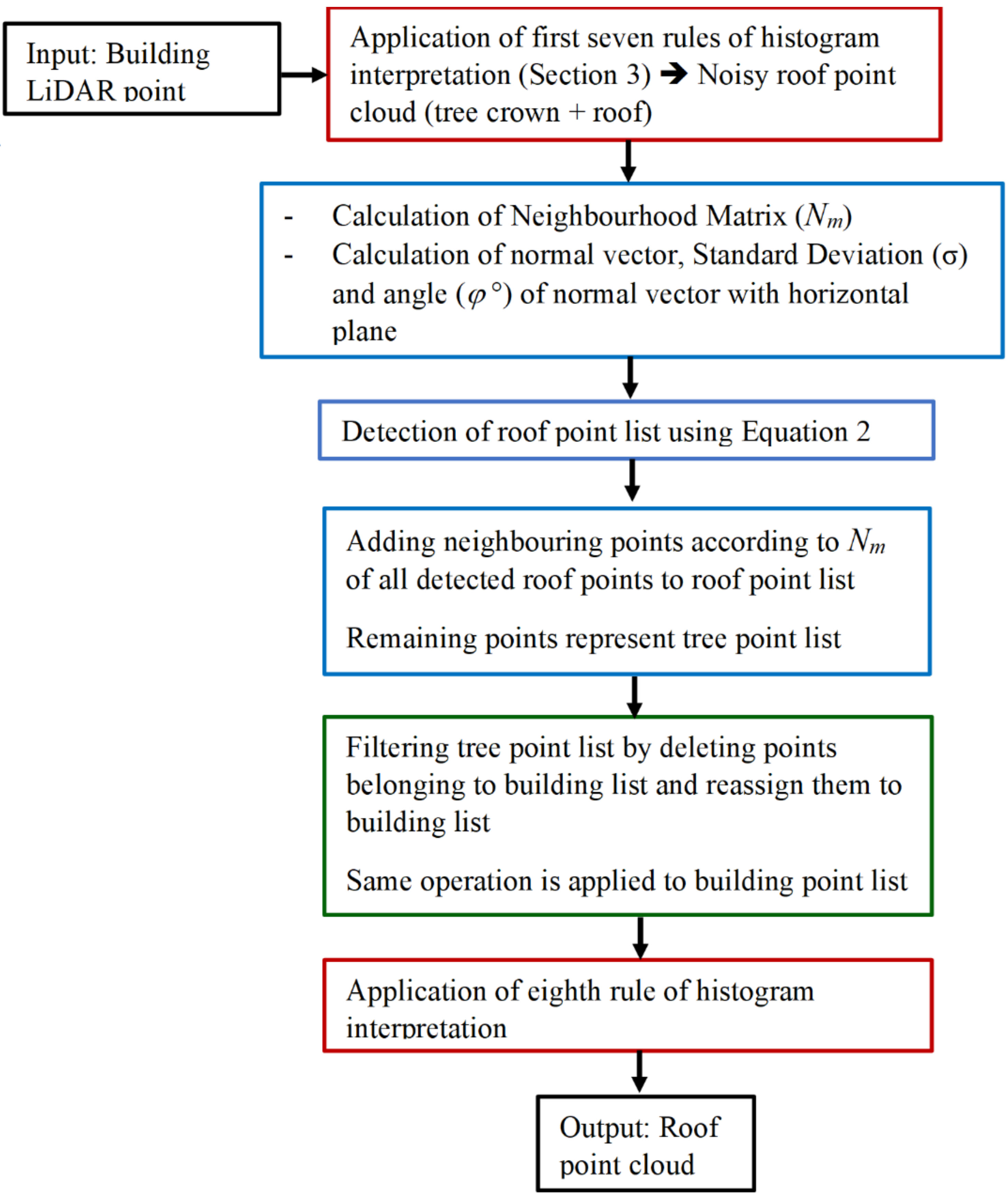
3. Filtering of Building Point Cloud Which Does Not Contain High Trees
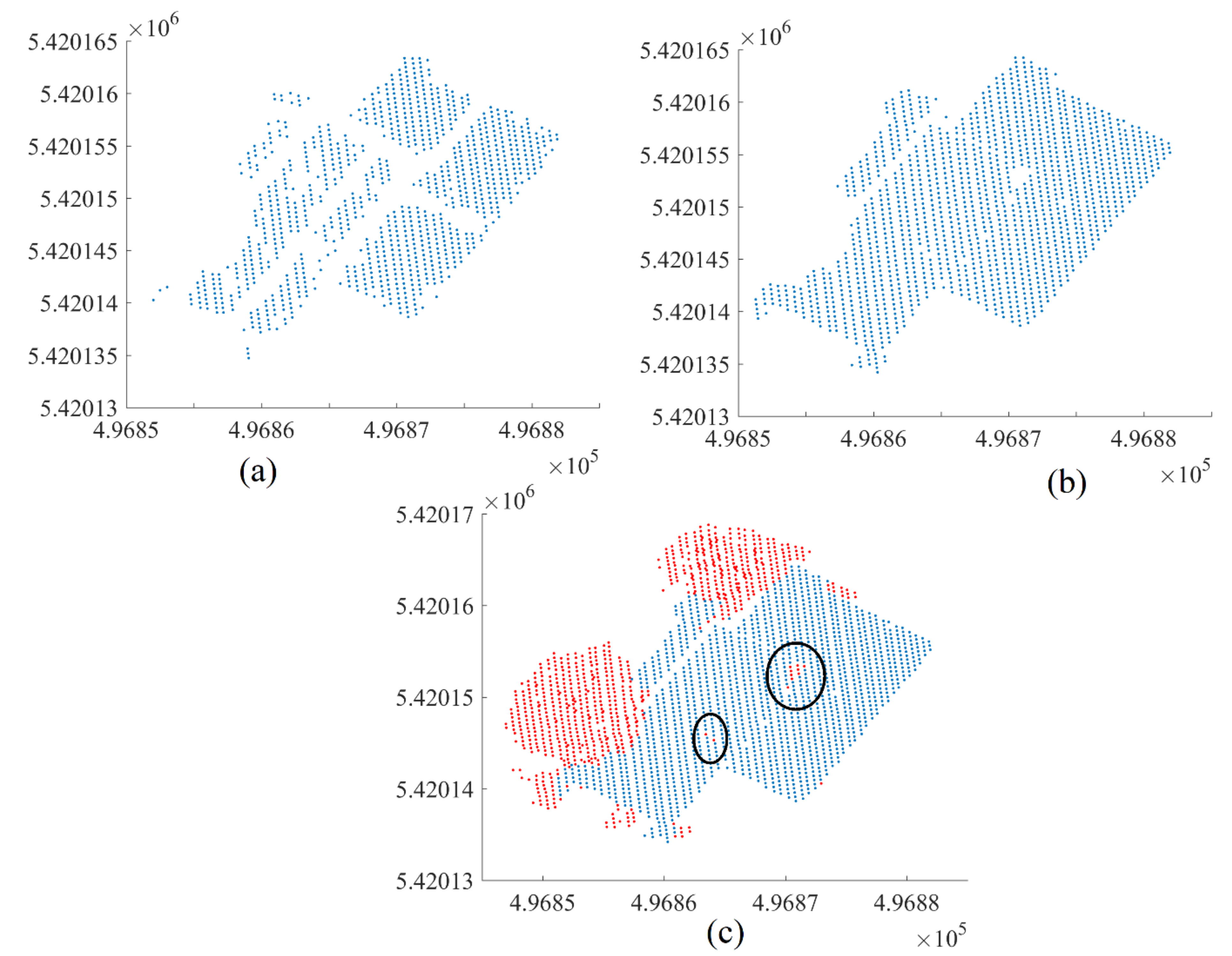
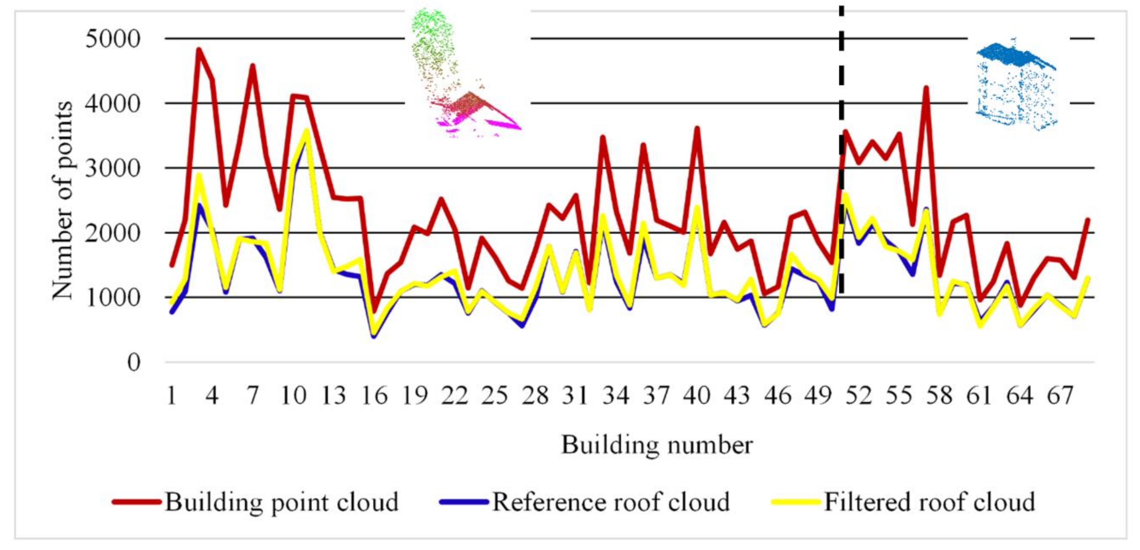
4. Results of Filtering Algorithm Application
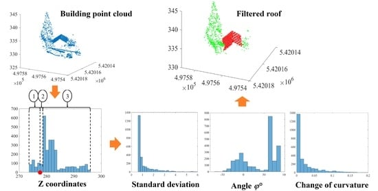
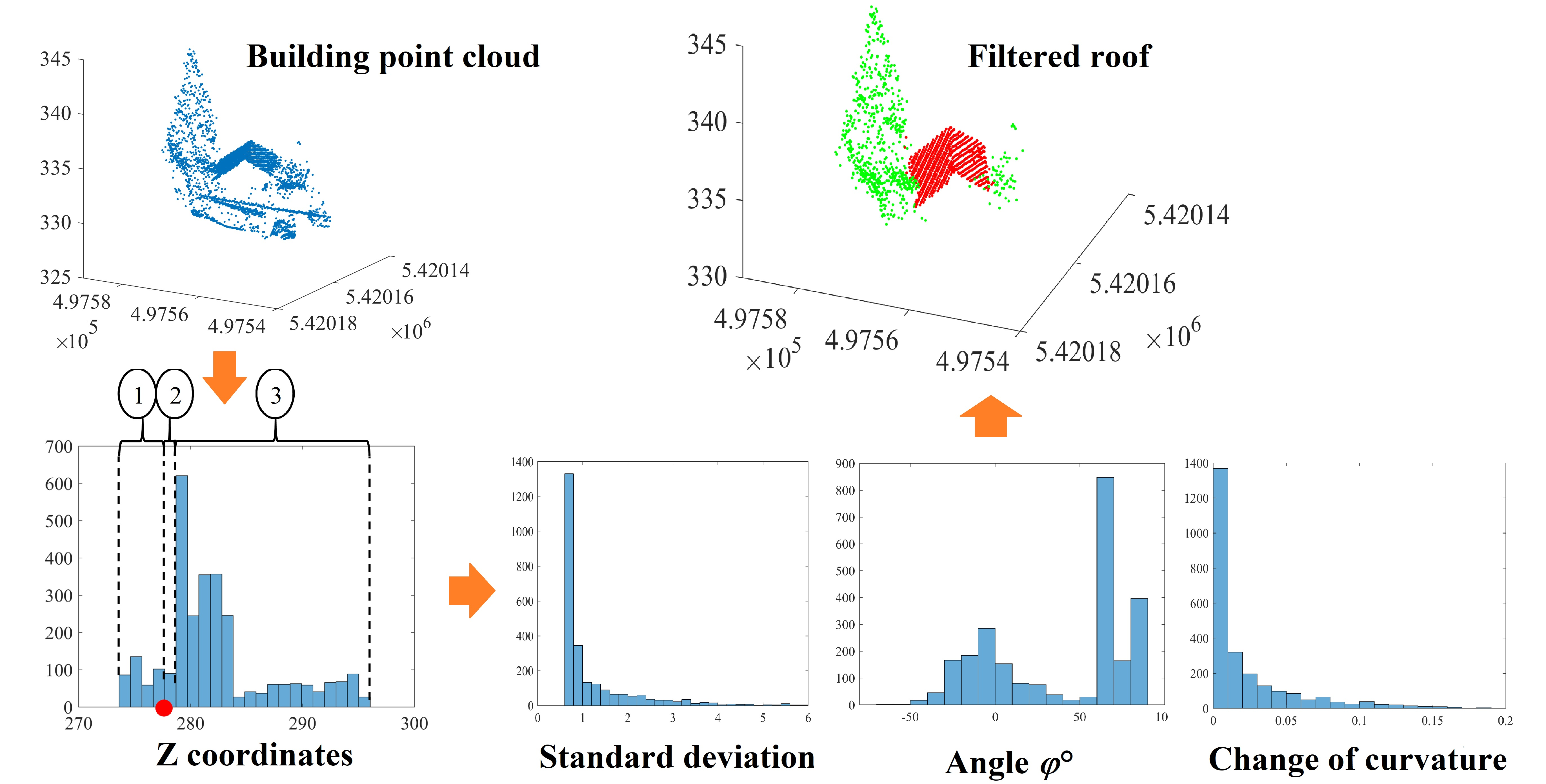
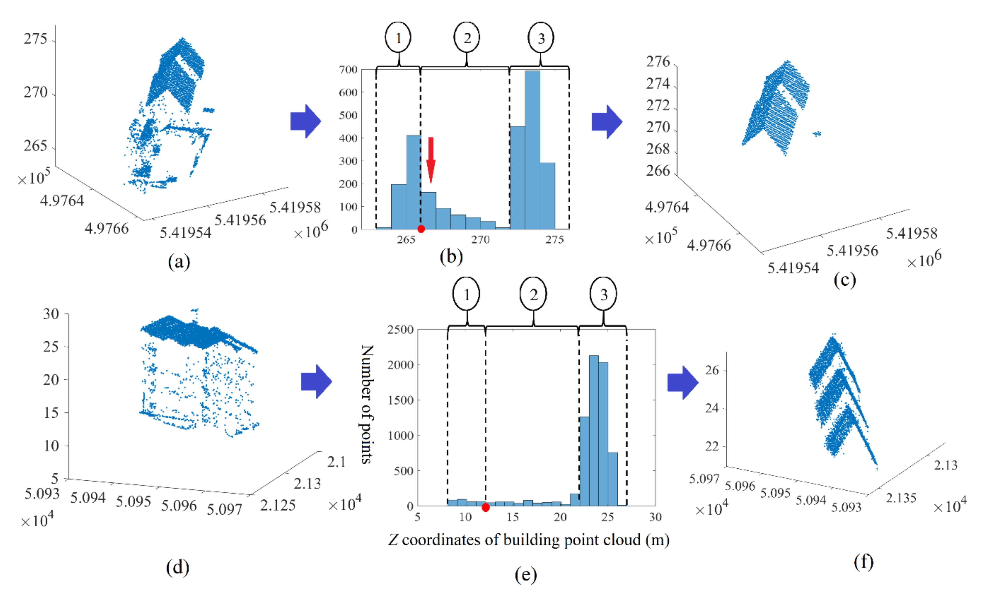
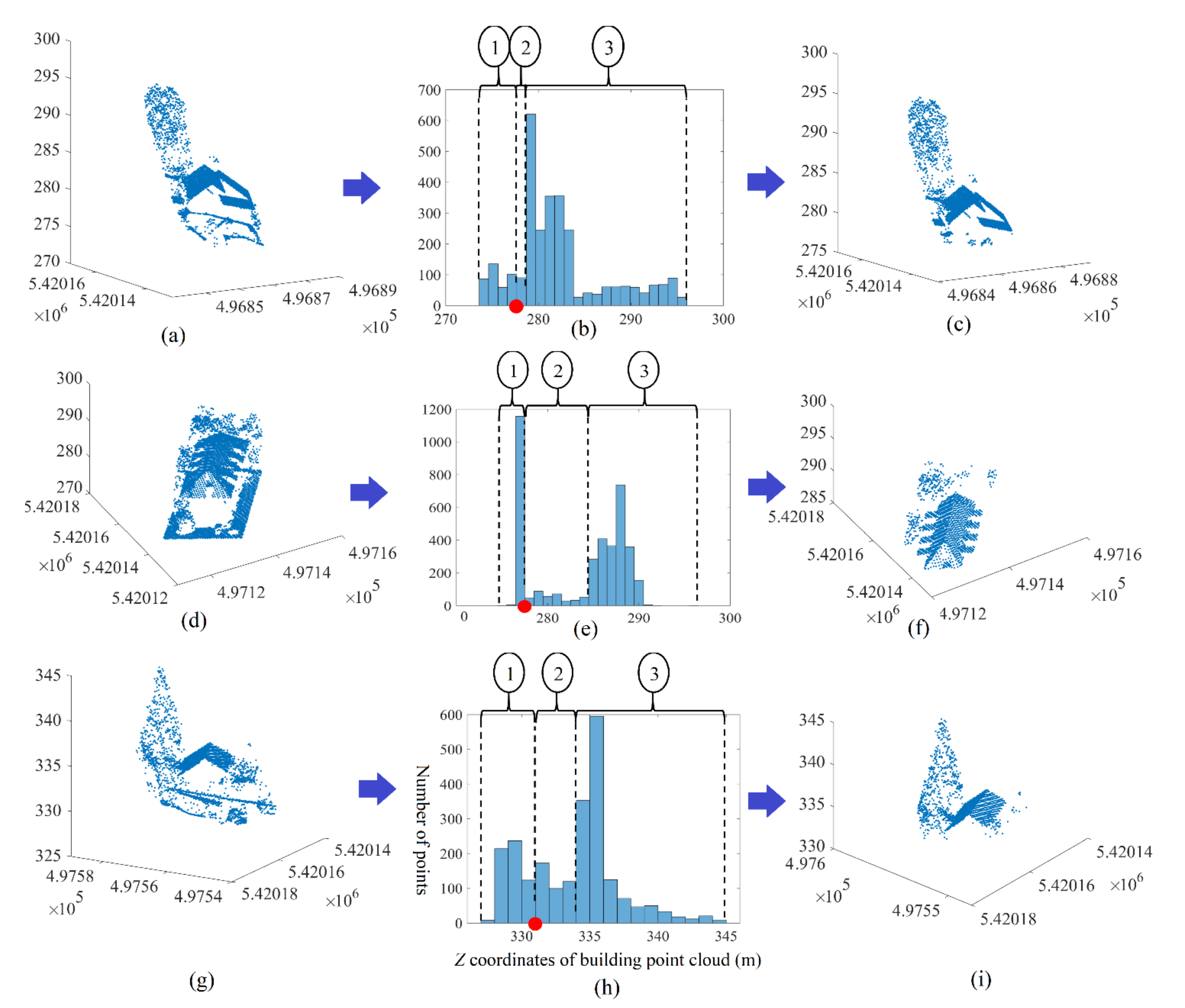
- The analysis of fuzzy bars in the building point cloud histogram has to be postponed to the end of the tree point elimination. This choice is supported by the fact that the roof planes, perhaps presented by fuzzy bars, are low in comparison to the building roof level and have smaller areas. If these planes were to be extracted before eliminating the tree points, they may be eliminated during the tree point recognition step.
- The application of the first seven rules on the building point cloud creates a new point cloud that represents the building roof (without the planes of fuzzy bars) in addition to the tree crown. This cloud will be named the noisy roof cloud.
5. Extended Filtering Algorithm
5.1. Selection of Neighbouring Points
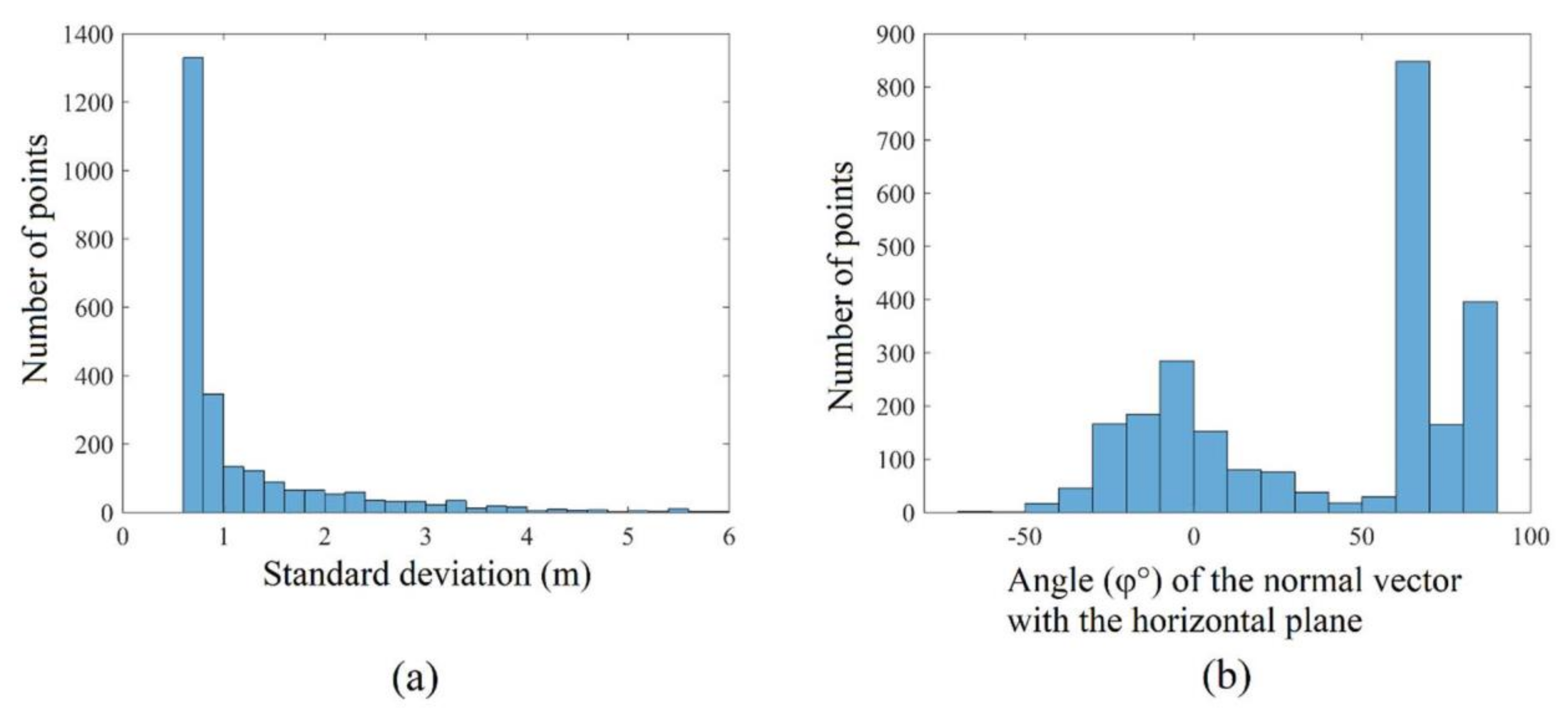
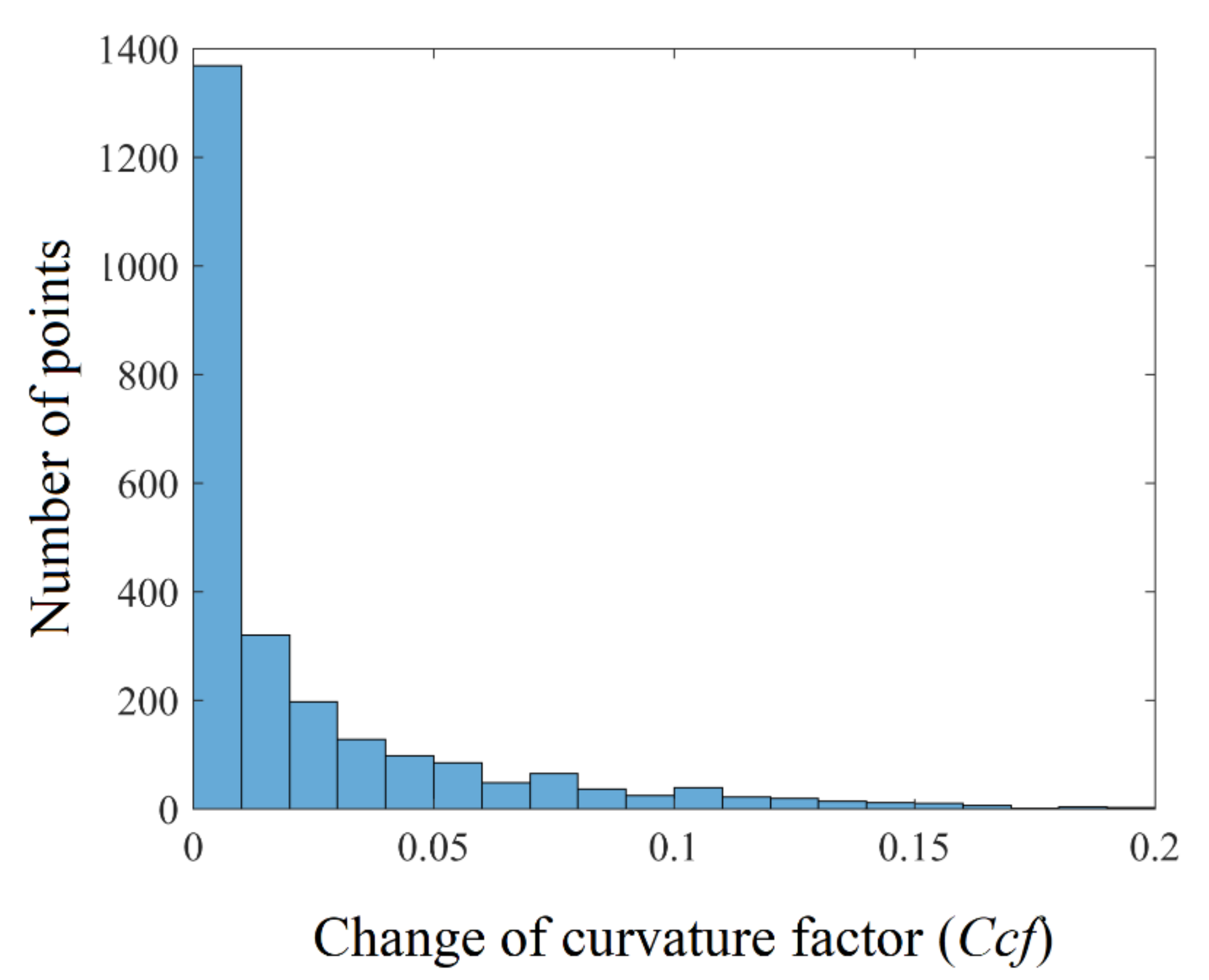
5.2. Calculation of Normal Vectors and Change of Curvature Factor
5.3. Filtering of Noisy Roof Point Cloud
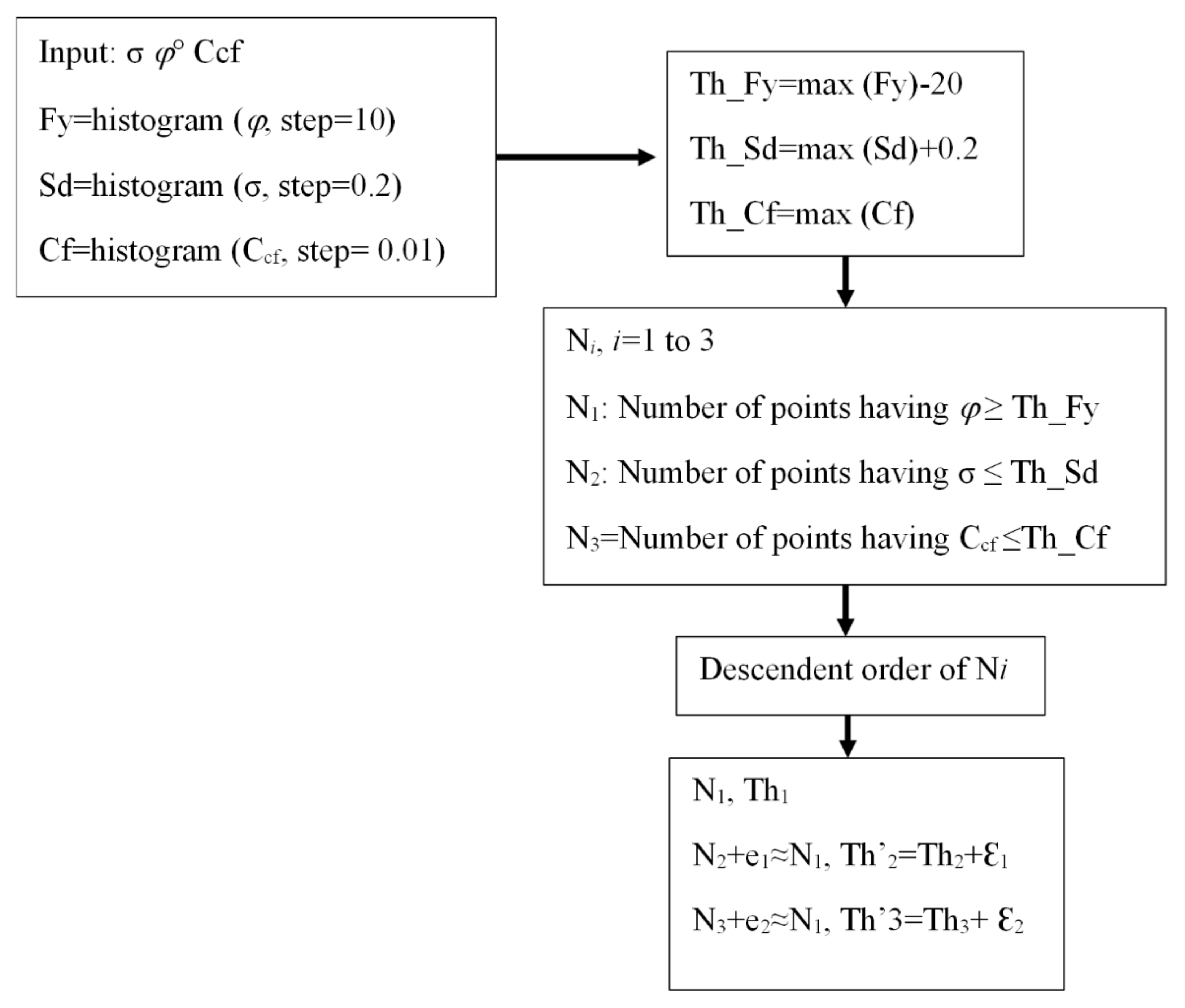
5.4. Calculation of Smart Threshold Values
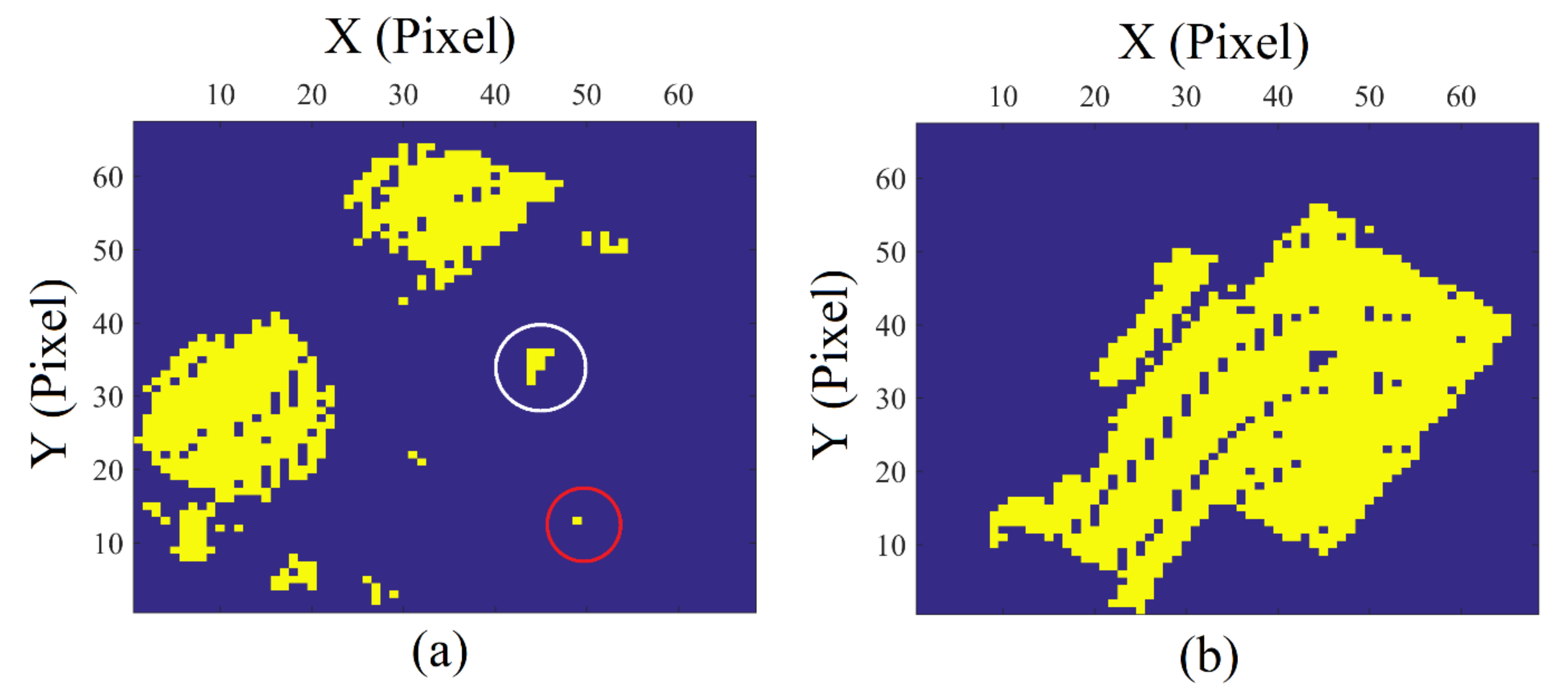
5.5. Improvement of Filtering Results
6. Results
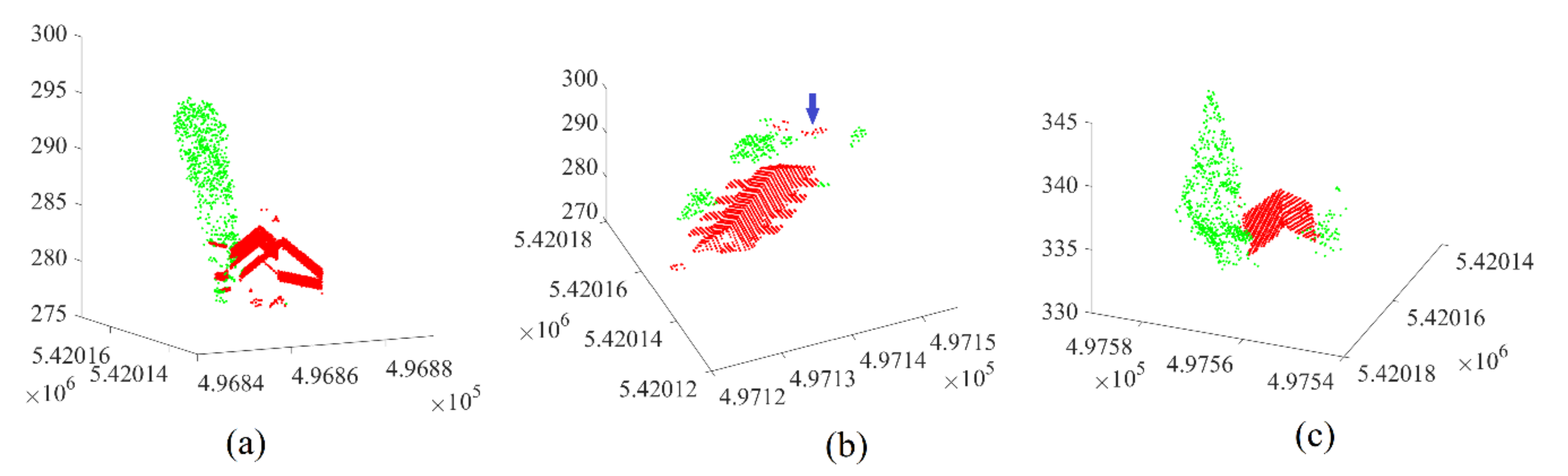
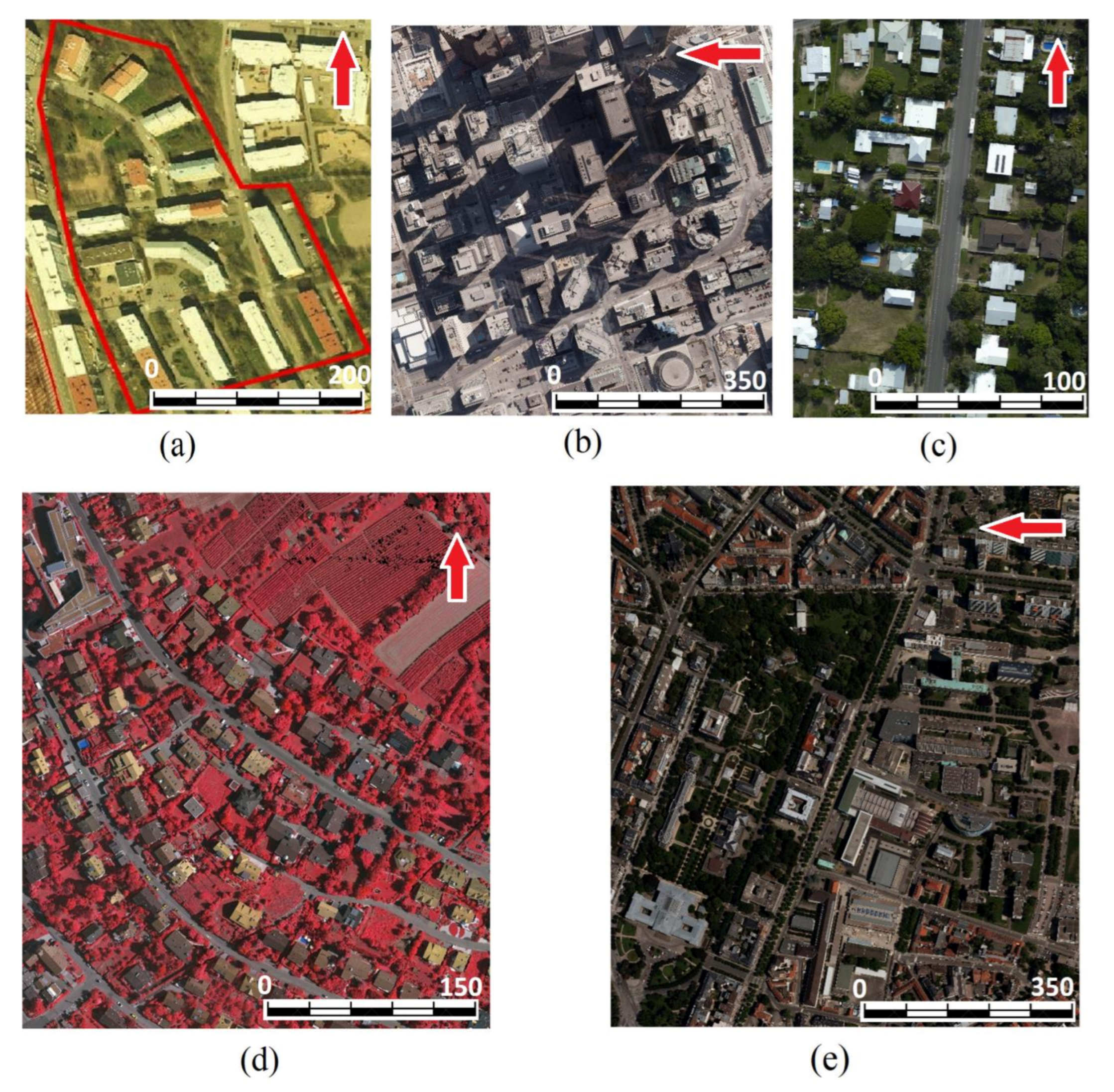
6.1. Datasets
6.2. Accuracy Estimation
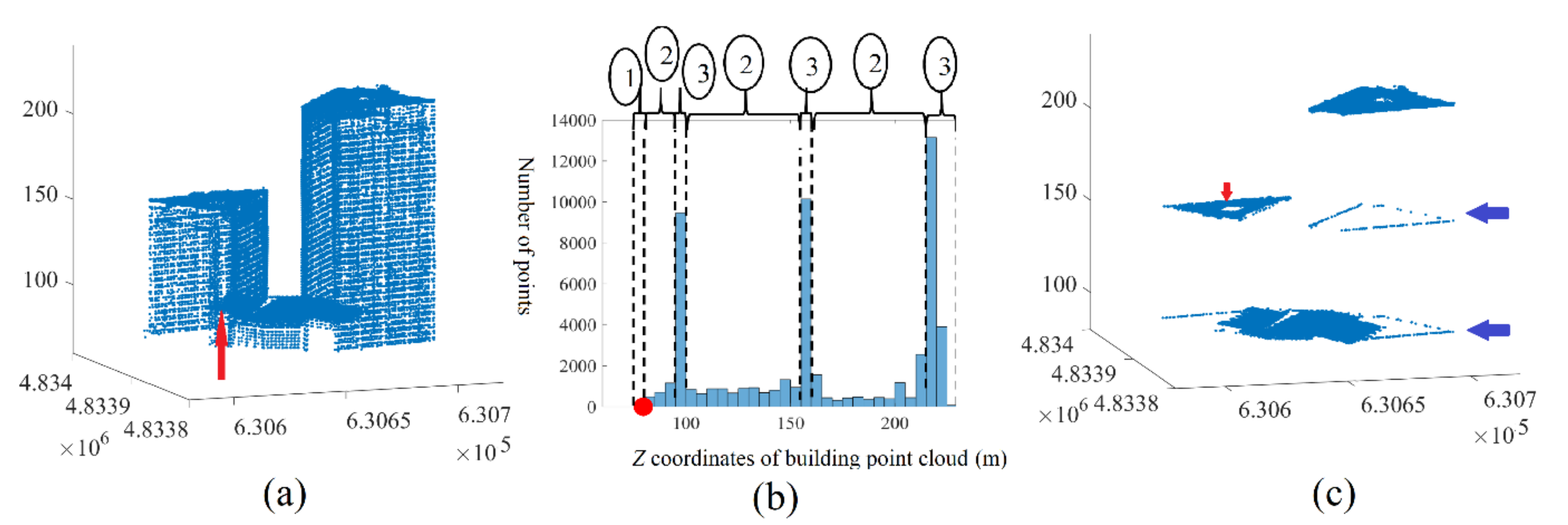
- In the case of high buildings with a high point density, the small roof planes that are not located in the main roof level may not be detected.
- In the case of buildings that consist of several masses with different heights, the portions of façade points with the same altitudes of the low roof planes will not be cancelled.
- Some of high tree points will not be eliminated.
7. Discussion
7.1. Filtering Accuracy Discussion
7.2. Accuracy Comparison
7.3. Comparison with Deep-Learning-Based Methods
7.4. Ablation Study
8. Conclusions and Perspective
Author Contributions
Funding
Institutional Review Board Statement
Informed Consent Statement
Data Availability Statement
Acknowledgments
Conflicts of Interest
References
- Shan, J.; Yan, J.; Jiang, W. Global Solutions to Building Segmentation and Reconstruction. Topographic Laser Ranging and Scanning: Principles and Processing, 2nd ed.; Shan, J., Toth, C.K., Eds.; CRC Press: Boca Raton, FL, USA, 2018; pp. 459–484. [Google Scholar]
- Tarsha Kurdi, F.; Landes, T.; Grussenmeyer, P.; Koehl, M. Model-driven and data-driven approaches using Lidar data: Analysis and comparison. In Proceedings of the ISPRS Workshop, Photogrammetric Image Analysis (PIA07), International Archives of Photogrammetry, Remote Sensing and Spatial Information Systems. Munich, Germany, 19–21 September 2007; 2007; Volume XXXVI, pp. 87–92, Part3 W49A. [Google Scholar]
- Wehr, A.; Lohr, U. Airborne laser scanning—An introduction and overview. ISPRS J. Photogramm. Remote Sens. 1999, 54, 68–82. [Google Scholar] [CrossRef]
- He, Y. Automated 3D Building Modelling from Airborne Lidar Data. Ph.D. Thesis, University of Melbourne, Melbourne, Australia, 2015. [Google Scholar]
- Tarsha Kurdi, F.; Awrangjeb, M. Comparison of Lidar building point cloud with reference model for deep comprehension of cloud structure. Can. J. Remote Sens. 2020, 46, 603–621. [Google Scholar] [CrossRef]
- Shao, J.; Zhang, W.; Shen, A.; Mellado, N.; Cai, S.; Luo, L.; Wang, N.; Yan, G.; Zhou, G. Seed point set-based building roof extraction from airborne LiDAR point clouds using a top-down strategy. Autom. Constr. 2021, 126, 103660. [Google Scholar] [CrossRef]
- Wen, C.; Li, X.; Yao, X.; Peng, L.; Chi, T. Airborne LiDAR point cloud classification with global-local graph attention convolution neural network. ISPRS J. Photogramm. Remote Sens. 2021, 173, 181–194. [Google Scholar] [CrossRef]
- Varlik, A.; Uray, F. Filtering airborne LIDAR data by using fully convolutional networks. Surv. Rev. 2021, 1–11. [Google Scholar] [CrossRef]
- Hui, Z.; Li, Z.; Cheng, P.; Ziggah, Y.Y.; Fan, J. Building extraction from airborne LiDAR data based on multi-constraints graph segmentation. Remote Sens. 2021, 13, 3766. [Google Scholar] [CrossRef]
- Tarsha Kurdi, F.; Awrangjeb, M.; Munir, N. Automatic filtering and 2D modelling of Lidar building point cloud. Trans. GIS J. 2021, 25, 164–188. [Google Scholar] [CrossRef]
- Maltezos, E.; Doulamis, A.; Doulamis, N.; Ioannidis, C. Building extraction from LiDAR data applying deep convolutional neural networks. IEEE Geosci. Remote Sens. Lett. 2019, 16, 155–159. [Google Scholar] [CrossRef]
- Liu, M.; Shao, Y.; Li, R.; Wang, Y.; Sun, X.; Wang, J.; You, Y. Method for extraction of airborne LiDAR point cloud buildings based on segmentation. PLoS ONE 2020, 15, e0232778. [Google Scholar] [CrossRef]
- Demir, N. Automated detection of 3D roof planes from Lidar data. J. Indian Soc. Remote Sens. 2018, 46, 1265–1272. [Google Scholar] [CrossRef]
- Tarsha Kurdi, F.; Awrangjeb, M.; Munir, N. Automatic 2D modelling of inner roof planes boundaries starting from Lidar data. In Proceedings of the 14th 3D GeoInfo 2019, Singapore, 26–27 September 2019; pp. 107–114. [Google Scholar] [CrossRef] [Green Version]
- Park, S.Y.; Lee, D.G.; Yoo, E.J.; Lee, D.C. Segmentation of Lidar data using multilevel cube code. J. Sens. 2019, 2019, 4098413. [Google Scholar] [CrossRef]
- Zhang, K.; Yan, J.; Chen, S.C. A framework for automated construction of building models from airborne Lidar measurements. In Topographic Laser Ranging and Scanning: Principles and Processing, 2nd ed.; Shan, J., Toth, C.K., Eds.; CRC Press: Boca Raton, FL, USA, 2018; pp. 563–586. [Google Scholar]
- Li, M.; Rottensteiner, F.; Heipke, C. Modelling of buildings from aerial Lidar point clouds using TINs and label maps. ISPRS J. Photogramm. Remote Sens. 2019, 154, 127–138. [Google Scholar] [CrossRef]
- Vosselman, G.; Dijkman, S. 3D building model reconstruction from point clouds and ground plans. Int. Arch. Photogramm. Remote Sens. Spat. Inf. Sci. 2001, 34, 37–44. [Google Scholar]
- Hu, P.; Miao, Y.; Hou, M. Reconstruction of Complex Roof Semantic Structures from 3D Point Clouds Using Local Convexity and Consistency. Remote Sens. 2021, 13, 1946. [Google Scholar] [CrossRef]
- Nguyen, T.H.; Daniel, S.; Guériot, D.; Sintès, C.; Le Caillec, J.-M. Super-Resolution-Based Snake Model—An Unsupervised Method for Large-Scale Building Extraction Using Airborne LiDAR Data and Optical Image. Remote Sens. 2020, 12, 1702. [Google Scholar] [CrossRef]
- Zhang, W.; Wang, H.; Chen, Y.; Yan, K.; Chen, M. 3D building roof modelling by optimizing primitive’s parameters using constraints from Lidar data and aerial imagery. Remote Sens. 2014, 6, 8107–8133. [Google Scholar] [CrossRef] [Green Version]
- Jung, J.; Sohn, G. Progressive modelling of 3D building rooftops from airborne Lidar and imagery. In Topographic Laser Ranging and Scanning: Principles and Processing, 2nd ed.; Shan, J., Toth, C.K., Eds.; CRC Press: Boca Raton, FL, USA, 2018; pp. 523–562. [Google Scholar]
- Awrangjeb, M.; Gilani, S.A.N.; Siddiqui, F.U. An effective data-driven method for 3D building roof reconstruction and robust change detection. Remote Sens. 2018, 10, 1512. [Google Scholar] [CrossRef] [Green Version]
- Pirotti, F.; Zanchetta, C.; Previtali, M.; Della Torre, S. Detection of building roofs and façade from aerial laser scanning data using deep learning. ISPRS-Int. Arch. Photogramm. Remote Sens. Spat. Inf. Sci. 2019, 4211, 975–980. [Google Scholar] [CrossRef] [Green Version]
- Martin-Jimenez, J.; Del Pozo, S.; Sanchez-Aparicio, M.; Laguela, S. Multi-scale roof characterization from Lidar data and aerial orthoimagery: Automatic computation of building photovoltaic capacity. J. Autom. Constr. 2020, 109, 102965. [Google Scholar] [CrossRef]
- Sibiya, M.; Sumbwanyambe, M. An algorithm for severity estimation of plant leaf diseases by the use of colour threshold image segmentation and fuzzy logic inference: A proposed algorithm to update a “Leaf Doctor” application. AgriEngineering 2019, 1, 205–219. [Google Scholar] [CrossRef] [Green Version]
- Dey, K.E.; Tarsha Kurdi, F.; Awrangjeb, M.; Stantic, B. Effective Selection of Variable Point Neighbourhood for Feature Point Extraction from Aerial Building Point Cloud Data. Remote Sens. 2021, 13, 1520. [Google Scholar] [CrossRef]
- Sanchez, J.; Denis, F.; Coeurjolly, D.; Dupont, F.; Trassoudaine, L.; Checchin, P. Robust normal vector estimation in 3D point clouds through iterative principal component analysis. ISPRS J. Photogramm. Remote Sens. 2020, 163, 18–35. [Google Scholar] [CrossRef] [Green Version]
- Thomas, H.; Goulette, F.; Deschaud, J.; Marcotegui, B.; LeGall, Y. Semantic Classification of 3D Point Clouds with Multiscale Spherical Neighborhoods. In Proceedings of the International Conference on 3D Vision (3DV), Verona, Italy, 5–8 September 2018; pp. 390–398. [Google Scholar] [CrossRef] [Green Version]
- Tarsha Kurdi, F.; Landes, T.; Grussenmeyer, P. Joint combination of point cloud and DSM for 3D building reconstruction using airborne laser scanner data. In Proceedings of the 4th IEEE GRSS / WG III/2+5, VIII/1, VII/4 Joint Workshop on Remote Sensing & Data Fusion over Urban Areas and 6th International Symposium on Remote Sensing of Urban Areas, Télécom, Paris, France, 11–13 April 2007; p. 7. [Google Scholar]
- Eurosdr. Available online: www.eurosdr.net (accessed on 23 November 2021).
- Cramer, M. The DGPF test on digital aerial camera evaluation—Overview and test design. Photogramm.-Fernerkund.-Geoinf. 2010, 2, 73–82. [Google Scholar] [CrossRef]
- Awrangjeb, M.; Zhang, C.; Fraser, C.S. Automatic extraction of building roofs using LiDAR data and multispectral imagery. ISPRS J. Photogramm. Remote Sens. 2013, 83, 1–18. [Google Scholar] [CrossRef] [Green Version]
- Huang, R.; Yang, B.; Liang, F.; Dai, W.; Li, J.; Tian, M.; Xu, W. A top-down strategy for buildings extraction from complex urban scenes using airborne LiDAR point clouds. Infrared Phys. Technol. 2018, 92, 203–218. [Google Scholar] [CrossRef]
- Widyaningrum, E.; Gorte, B.; Lindenbergh, R. Automatic Building Outline Extraction from ALS Point Clouds by Ordered Points Aided Hough Transform. Remote Sens. 2019, 11, 1727. [Google Scholar] [CrossRef] [Green Version]
- Zhao, Z.; Duan, Y.; Zhang, Y.; Cao, R. Extracting buildings from and regularizing boundaries in airborne LiDAR data using connected operators. Int. J. Remote Sens. 2016, 37, 889–912. [Google Scholar] [CrossRef]
- Griffiths, D.; Boehm, J. Improving public data for building segmentation from Convolutional Neural Networks (CNNs) for fused airborne lidar and image data using active contours. ISPRS J. Photogramm. Remote Sens. 2019, 154, 70–83. [Google Scholar] [CrossRef]
- Ayazi, S.M.; Saadat Seresht, M. Comparison of traditional and machine learning base methods for ground point cloud labeling. Int. Arch. Photogramm. Remote Sens. Spatial Inf. Sci. 2019, XLII-4/W18, 141–145. [Google Scholar] [CrossRef] [Green Version]


| Thφ (Degree) | Thσ (m) | Thccf (Unitless) | |
|---|---|---|---|
| Building 1 | 40 | 0.8 | 0.01 |
| Building 2 | 30 | 0.8 | 0.04 |
| Building 3 | 50 | 0.8 | 0.02 |
| Building 4 | 30 | 0.9 | 0.03 |
| Building 5 | 30 | 0.8 | 0.02 |
| Building 6 | 40 | 0.8 | 0.02 |
| Building 7 | 30 | 0.8 | 0.01 |
| Building 8 | 45 | 0.8 | 0.02 |
| Building 9 | 30 | 0.8 | 0.02 |
| Hermanni | Strasbourg | Toronto | Vaihingen | Aitkenvale | |
|---|---|---|---|---|---|
| Acquisition | June 2002 | September 2004 | February 2009 | August 2008 | -- |
| Sensor | TopoEye | TopScan (Optech ALTM 1225) | Optech ALTM-ORION M | Leica Geosystems (Leica ALS50) | -- |
| Point density (point/m2) | 7–9 | 1.3 | 6 | 4–6.7 | 29–40 |
| Flight height (m) | 200 | 1440 | 650 | 500 | >100 |
| Dataset | Number of Buildings | Number of Points | Undesirable Points (%) | Corr (%) | Comp (%) | Q (%) |
|---|---|---|---|---|---|---|
| Average Values | ||||||
| Hermanni | 12 | 7380 | 13.37 | 99.69 | 99.76 | 99.45 |
| Strasbourg | 56 | 1433 | 18.05 | 98.44 | 95.63 | 94.24 |
| Toronto | 72 | 14,700 | 23.25 | 98.56 | 95.57 | 94.23 |
| Vaihingen | 68 | 2542 | 41.65 | 94.85 | 98.39 | 93.37 |
| Aitkenvale | 28 | 9822 | 37.1 | 98.1 | 98.75 | 96.93 |
| Average | 7175 | 26.7 | 97.9 | 97.6 | 95.6 | |
| Corr (%) | Comp (%) | Q (%) | |
|---|---|---|---|
| Maltezos et al. [11] | 85.3 | 93.8 | 80.8 |
| Widyaningrum et al. [35] | 90.1 | 99.4 | 89.6 |
| Huang et al. [34] | 96.8 | 96.2 | 93.2 |
| Zhao et al. [36] | 91.0 | 95.0 | 86.8 |
| Hui et al. [9] | 91.61 | 93.61 | 85.74 |
| Wen et al. [7] | 95.1 | 91.2 | 86.7 |
| Suggested approach | 97.9 | 97.6 | 95.6 |
| Total Build | Z_His | φ° | σ | ccf | φ°+ σ + ccf | Nm | Imp | Fuz | Roof | Tree | Und |
|---|---|---|---|---|---|---|---|---|---|---|---|
| 2936 | 2503 | 1456 | 1329 | 1368 | 1065 | 597 | 14 | 55 | 1727 | 776 | 433 |
Publisher’s Note: MDPI stays neutral with regard to jurisdictional claims in published maps and institutional affiliations. |
© 2022 by the authors. Licensee MDPI, Basel, Switzerland. This article is an open access article distributed under the terms and conditions of the Creative Commons Attribution (CC BY) license (https://creativecommons.org/licenses/by/4.0/).
Share and Cite
Tarsha Kurdi, F.; Gharineiat, Z.; Campbell, G.; Awrangjeb, M.; Dey, E.K. Automatic Filtering of Lidar Building Point Cloud in Case of Trees Associated to Building Roof. Remote Sens. 2022, 14, 430. https://doi.org/10.3390/rs14020430
Tarsha Kurdi F, Gharineiat Z, Campbell G, Awrangjeb M, Dey EK. Automatic Filtering of Lidar Building Point Cloud in Case of Trees Associated to Building Roof. Remote Sensing. 2022; 14(2):430. https://doi.org/10.3390/rs14020430
Chicago/Turabian StyleTarsha Kurdi, Fayez, Zahra Gharineiat, Glenn Campbell, Mohammad Awrangjeb, and Emon Kumar Dey. 2022. "Automatic Filtering of Lidar Building Point Cloud in Case of Trees Associated to Building Roof" Remote Sensing 14, no. 2: 430. https://doi.org/10.3390/rs14020430