1. Introduction
It is widely recognized that tropospheric water vapor (WV), which represents about 99% of the total WV, is of paramount importance in meteorology [
1,
2,
3,
4]. As a matter of fact, the amount of water available for precipitation in any form depends on its global and local dynamics. Furthermore, the transformation of the water from the gas phase to the liquid phase—and vice versa—produces the release and absorption of energy in the form of latent heat and, thus, it affects the thermic profiles of the atmosphere, which are at the basis of the atmospheric transport processes. Therefore, the measure of the WV concentration and of its variation as a function of the altitude is essential to guarantee a correct forecast of the rainfall and of the related atmospheric phenomena. However, achieving appropriate resolution and sensitivity to measure the time and spatial (both vertical and horizontal) variations of WV still represents a challenging goal [
5,
6,
7]. Furthermore, it is recognized that to precisely represent the global water cycle, a large number of observations is needed as input to atmospheric models [
8].
There are several methods to estimate the atmospheric WV content. Roughly speaking, they can be classified into methods that measure the local content of humidity—e.g., in situ methods that provide vertical profiles of WV through radio soundings (possibly in combination with Raman lidar measurements or even through standalone lidars, see for instance [
9])—and methods, both active and passive, which estimate the WV remotely through the sensitivity of an electromagnetic signal to the WV content at different frequencies. The former methods are the most precise techniques to measure the WV concentration, but they are an expensive solution and they do not allow for continuous time-spatial measures, as only spaceborne systems may guarantee them. The latter methods are real remote sensing techniques, which can be implemented on satellites, thus providing global coverage: they are based either on ground radiometers working in the infrared spectrum [
10] or on the phase difference of signals sent by global navigation satellite systems (GNSS)—such as GPS, Galileo, GLONASS, BeiDou—and measured by fixed stations [
2]. This second class of methods is able to provide the average WV content along the electromagnetic path of the sounding signals or, using a specific tomographic approach, also to provide estimates of water vapor above a network of receivers [
11,
12]. Average vertical profiles of the WV concentration over an area are provided by specific inversion techniques of such signals by Radio Occultation (RO) methods, with the aid of independent auxiliary information [
13]. Other kind of methods have been proposed to observe WV even from geostationary satellites by exploiting infrared measurements [
14], or to utilize spaceborne differential absorption radars to provide the columnar WV content, which is a key parameter in numerical prediction models (NWP) [
15].
All the global monitoring systems available at present, however, suffer from an accuracy issue of the WV measurements in the lower troposphere where, on the other hand, the WV concentration is maximum [
5].
A measurement approach that has the potential to overcome such an issue has been proposed some years ago. It is based on the so-called Normalized Differential Spectral Attenuation (NDSA) method applied to microwave links established between two Low Earth Orbiting (LEO) satellites [
16]. The NDSA method enables one to get estimates of the integrated water vapor (IWV, intended as absolute mass of water vapor) along such links; by means of specific inversion methods, WV concentration (intended as absolute humidity) profiles or fields can then, in turn, be estimated. Being based on limb soundings of the troposphere, such an approach gains more sensitivity to the presence of WV in the lower layers with respect to other kinds of measurements from space. The NDSA approach is characterized by a certain simplicity
per se. It requires the measurement of a parameter called spectral sensitivity, which is the normalized incremental ratio of the spectral attenuation at a given frequency. This turns out to be a quite simple function of the received powers of two simultaneously transmitted sinusoidal signals which travel from the transmitter (Tx) onboard a first LEO satellite to the receiver (Rx) onboard a second one. The frequencies of the signals are very close to each other, as their difference is about two orders of magnitude smaller than their average frequency, which is conventionally taken as the “channel” of the spectral sensitivity measurement. As shown in [
16] and [
17], which the reader is referred to for details, the spectral sensitivity is highly correlated to the IWV if frequency channels in the Ku-K bands are employed, so that the IWV pertaining to the Tx-Rx link can be estimated through simple pre-set linear relationships. Furthermore, being the spectral sensitivity based on normalized incremental measures, the NDSA approach limits the negative effects of tropospheric scintillation [
18]. In a multichannel (i.e., multifrequency) approach, higher frequency bands can be used both to estimate WV in the upper tropospheric layers and to detect the presence of liquid water along the radio path, giving the possibility to correct the bias it generates on WV estimates [
16,
19].
As pointed out in [
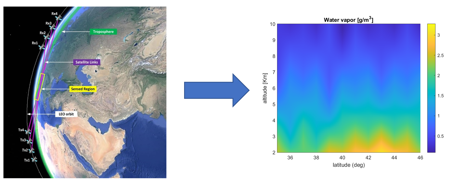
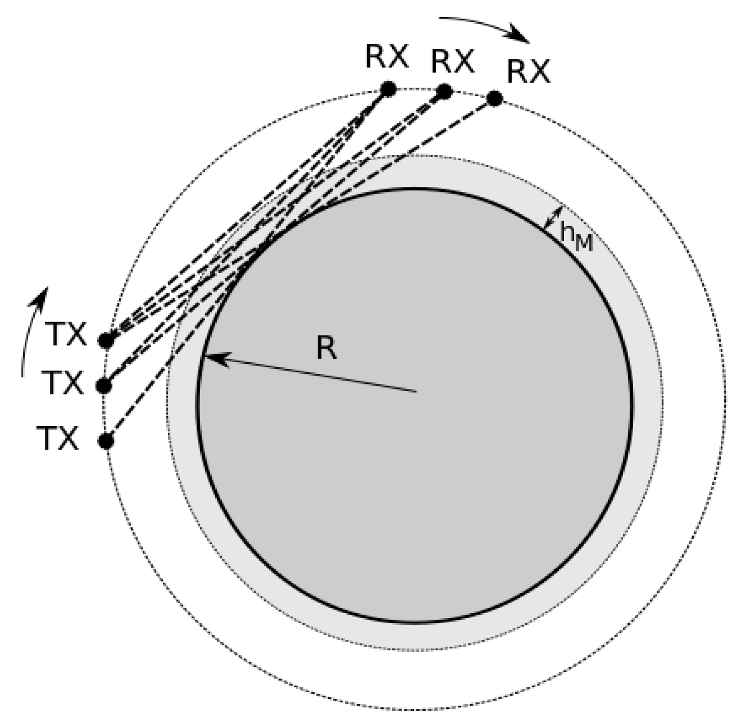
17], where the authors aimed at estimating the accuracy with which the spectral sensitivity is measured at different tangent altitudes of the Tx-Rx link, the NDSA approach can be exploited both in a “counter-rotating” configuration and in a “co-rotating” one. In the former case, a couple of LEO satellites orbit in the same plane and in opposite directions, thus having relative sunrises or sunsets. A vertical IWV profile is obtained over a certain position of the Earth, and the WV profile can be obtained by proper inversion methods. In the latter configuration, which is the case focused in this paper, we have a set of LEO satellites orbiting in the same plane and along the same direction: in this manner, one or more Tx LEO satellites chase a group of Rx LEO satellites so that they are always in view of each other, as illustrated in
Figure 1. The result is that there is a number of constantly active radio links that cross the troposphere at fixed tangent altitudes with respect to the Earth, covering and scanning an annular region of the orbital plane. The minimum and maximum altitude of such annular region are defined by the two microwave links with the minimum and maximum tangent altitude, respectively (For the sake of simplicity, we assume a spherical Earth so that the tangent altitude of each link does not vary.). Such a configuration of LEO satellites, whose realization is nowadays made easier with affordable costs thanks to the Cubesat technology, allows integration intervals longer than in the counter-rotating configuration (where the integration time is limited by the requested vertical resolution), with a clear benefit to reduce the noise and scintillation impacts at the receiver. In the co-rotating scenario, the set of IWV measurements collected during the observation time can be inverted to obtain the two-dimensional (2D) concentration of WV in the scanned annular region (i.e., on planes perpendicular to the Earth surface). In [
20], an inversion approach based on least squares minimization and Tikhonov regularization (in the following referred to as LSATR, i.e., Least Squares Algorithm with Tikhonov Regularization) was proposed. In this paper, we focus on an alternative approach of tomographic inversion that is perfectly coherent with the geometry of the inversion problem at hand and with the path-integrated nature of NDSA measurements; to the best of our knowledge, this technique has never been applied before in the field of remote sensing. Its original formulation, by Cormack, dates back to the ’60 [
21,
22] and has been revisited and analyzed in the following decades by Cormack himself [
23], Perry [
24] and Quinto [
25,
26,
27] with applications to radiology and non-destructive testing. The mathematical problem posed in [
21] is inverting the Radon transform of a 2D field calculated on a compact annular region. In our specific problem, the unknown 2D field to be retrieved is the WV concentration in the aforementioned annular region of the orbital plane of the LEO satellites while its Radon transform corresponds to the ensemble of IWV estimates made available by the time series of NDSA measurements. The nature of this inversion method—referred to as External Reconstruction Tomographic Algorithm (ERTA) in this paper—poses profoundly different problems with respect to LSATR, but also leads to quite different retrieval performances. Objective of this paper is investigating the application of the ERTA approach to the IWV measurements inversion scenario as well as comparing its performance with respect to the LSATR method. The analysis shown here is part of the study that been developed within the SATCROSS project funded by the Italian Space Agency (ASI), aimed at providing a feasibility study for future missions.
This paper is structured as follows. In
Section 2, we briefly recall the NDSA measurement approach and the geometry of the acquisition system, constituted by a constellation of co-rotating LEO satellites. In
Section 3, we introduce ERTA, based on the previous work by Cormack, Perry and Quinto, whereas in
Section 4 we present its specific application to our measurement scenario.
Section 5 shows some examples of WV retrieval by using both ERTA and LSATR in the presence of realistic signal impairments. In
Section 6, some concluding remarks are drawn.
2. The NDSA Measurement Concept
The NDSA technique, described in [
16] and [
17] (which the reader is referred to for details), is based on the conversion of the spectral sensitivity
to the total content of water vapor (IWV) along the propagation path between two LEO satellites, one with a transmitter onboard and the other with a receiver. Defining
A(f) as the total spectral attenuation undergone by a signal tone at frequency
f, the spectral sensitivity function is the normalized derivative of
A(f), that is
The spectral sensitivity
at a given frequency
is obtained by transmitting two sinusoidal signals at two close frequencies
and
(
), such that their distance
, referred to as “spectral separation”, does not exceed 2.2% of
. Under this hypothesis, and assuming also that the two transmit signals have the same power, the spectral sensitivity
S referred to
(pointed out as a subscript whenever needed) is simply the finite difference approximation of the spectral sensitivity function defined in Equation (1)
where
and
are the powers of the two received tones measured at the receiver.
In [
16] and [
19], the authors have shown that the IWV along a given radio path and the spectral sensitivity
S measured along that link are tightly related, so that one can estimate the IWV from the knowledge of
S by using specific IWV-S relationships. Such relationships have been computed in ideal conditions (i.e., no signal impairments) by means of a regression analysis, for different values of
fo and tangent altitudes, showing that for different intervals of tangent altitudes an optimal
fo exists for which the IWV-S relationships are tight. The analysis was carried out by using a large set of atmospheric profiles (temperature, pressure, and WV concentration) coming from available radiosonde observations (in [
16]) and from ECMWF (European Centre for Medium range Weather Forecasts) analysis data (in [
19]). Each of such profiles was in turn used to generate a spherically symmetric atmosphere. In brief, the procedure to derive IWV-S relationships accounting for the seasonal, daily and geographical variations of the atmospheric conditions was the following. For a given a profile (from radiosondes or ECMWF analysis data) and for a link at a given tangent altitude, we calculated the IWV by integrating the WV concentration along the path, while we computed
assuming that
P1 and
P2 were measured in ideal conditions. After having repeated this procedure for all available profiles, we obtained the optimal value of
fo and the corresponding coefficients of a linear IWV-S relationship for any tangent altitude below 10 km. The conclusion of such analysis was that the optimal frequencies to provide IWV measurements between two LEO satellites up to 11-km tangent altitude are 17, 19, and 21 GHz.
The Signal to Noise Ratio (SNR) at the receiver is one of the most important parameters that impact the measure of
. It increases with the integration time used to estimate
and
. Increasing the integration time, however, means a lower number of available measurements in a certain area and then a worse resolution in the IWV measurements. In particular, in the case of counter-rotating satellites, increasing the integration time limits the vertical resolution of the IWV. In [
17], it has been demonstrated that accurate measure of
can not be achieved with a SNR lower than 20 dB, which implies that the integration time has to be at least 10 ms. In the case of co-rotating satellites, which is the case analyzed in this paper, much higher integration times can be used, and this guarantees a greater accuracy in the estimate of the IWV.
3. The External Reconstruction Tomographic Algorithm (ERTA)
In this section, we summarize the basic mathematics of the so-called exterior reconstruction problem and show some outcomes of our implementation of the ERTA.
Let us denote the water vapor function to be reconstructed as
, expressed in polar coordinates. The measured IWV field coincides with its Radon Transform, indicated in the following as
and defined as
where
is a line identified by the couple (
ρ,), with
ρ the distance of
from the origin and
the angle formed by the
θ = 0 axis and the normal to the line. The inversion technique known as
Exterior Radon Transform has been introduced for the first time by Cormack, whose important contribution was the demonstration that the values of the function
can be uniquely retrieved from the knowledge of its Radon Transform
[
21]. Successively, the technique has been expanded in other works by Perry and Quinto [
24,
25,
26,
27]. In
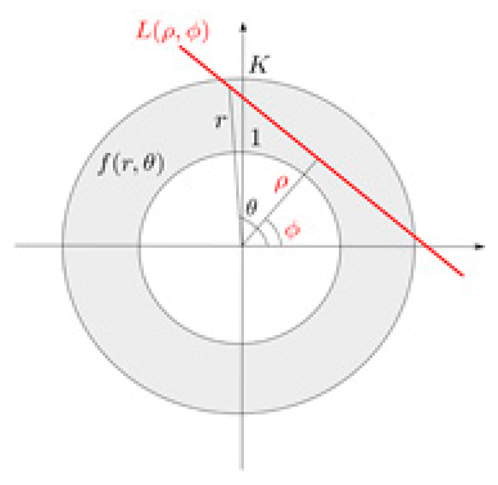
Figure 2, the geometry of the ERTA acquisition system is shown (in the figure, the radial distance
r is normalized with respect to the minimum possible radial distance
, i.e., the Earth radius in our case). Hence, the boundaries of the normalized interval [1,
K] correspond to
ro and to the maximum altitude of the annular region, respectively.
The functions
and
are periodical in the angle variables
and
, respectively, so that they can be expanded as Fourier series, that is
The first important theoretical result is that each term of the two series can be further decomposed by means of bases of functions, whose elements
and
,
, are described by Jacobi polynomials and whose major characteristic is that the Radon transform maps such functions onto each other [
24]. More specifically, consider the following definitions:
where
is an integer and
with
Jacobi polynomials and
where Γ(x) is the Euler Gamma function. If
denotes the Radon operator, then it can be demonstrated that
with
, while
denotes the integer part and
Such results demonstrate not only the previously mentioned mapping property of elements of the set onto elements of the set , but also a second important result of this tomographic approach, which is the existence of nonnull functions whose Radon transform is null. These functions generate the null space of the transform, denoted as SN. For similarity, the functions that produce a nonnull Radon transform will generate the nonnull space, referred to as SR. It is worth noting that in our problem the observable quantities are samples of the Radon transform, so that the null space cannot be reconstructed from the measurements; in other words, the null space may have a role in the reconstruction of the function only if some a priori knowledge is available (for example, if we knew that the solution is smooth).
The third important fact is that the elements
and
are orthogonal in the space domain and in the Radon domain, respectively, if particular weight functions are used to define the inner product in such spaces. More specifically, the Hilbert spaces which
and
belong to are composed by functions defined on
. The functions
and
are orthogonal in their respective spaces according to the following inner product
with weight function
in the space domain and
in the Radon domain.
The reconstruction algorithm, based only on the nonnull space S
R, starts with a decomposition of the acquired Radon transform
(the IWV measurements) by using the set of functions
, i.e.,
where
dn,l are the coefficients of the expansion. The coefficients
dn,l are computed according to Equation (13) which, expressed in polar coordinates, becomes
According to the mapping property in Equation (11) [
26], we have
where
denotes the function (belonging to S
R) that can be achieved from the Radon transform. It is worth noting that for each
-th angular Fourier expansion coefficient, all the terms of the expansion along
with index
, are transformed by the Radon operator into a null function: thus, the higher the frequency component index of the WV field to be reconstructed, the higher the number of radial basis functions that will not be reconstructed by the procedure (because they belong to the null space). The only coefficients of the angular Fourier series that are completely reconstructed by the procedure are those relative to the continuous and fundamental frequencies.
4. Application of the ERTA Approach to the Reconstruction of WV Fields
In this section, we analyze the peculiarities of the application of ERTA to the reconstruction of a WV field based on a constellation of LEO satellites and a set of NDSA measurements. As a matter of fact, there are significant differences with respect to the original applications of ERTA shown for instance in [
24,
25,
26,
27]. In fact, our setup is characterized by a very narrow annular region (if the width is compared to the inner radius) to be reconstructed and by a very limited number of links on which the IWV can be computed, due to the complexity of the deployment of a highly populated constellation of satellites. Furthermore, the underlying function to be reconstructed (i.e., the 2D WV field) is expected to be quite regular (and in any case, so are the 2D WV fields generated by numerical prediction models that have been used as ‘truth’ reference in our simulations). This has an impact on the choice of the parameters of the ERTA implementation (for instance, the number of polynomials).
To better illustrate the ERTA potential outcomes, we first present and discuss the retrieval results in an ideal case (i.e., in the absence of any impairment source), leaving to
Section 5 the analysis in the presence of disturbances. We consider as ‘true map’ the same atmospheric scenario that we used in [
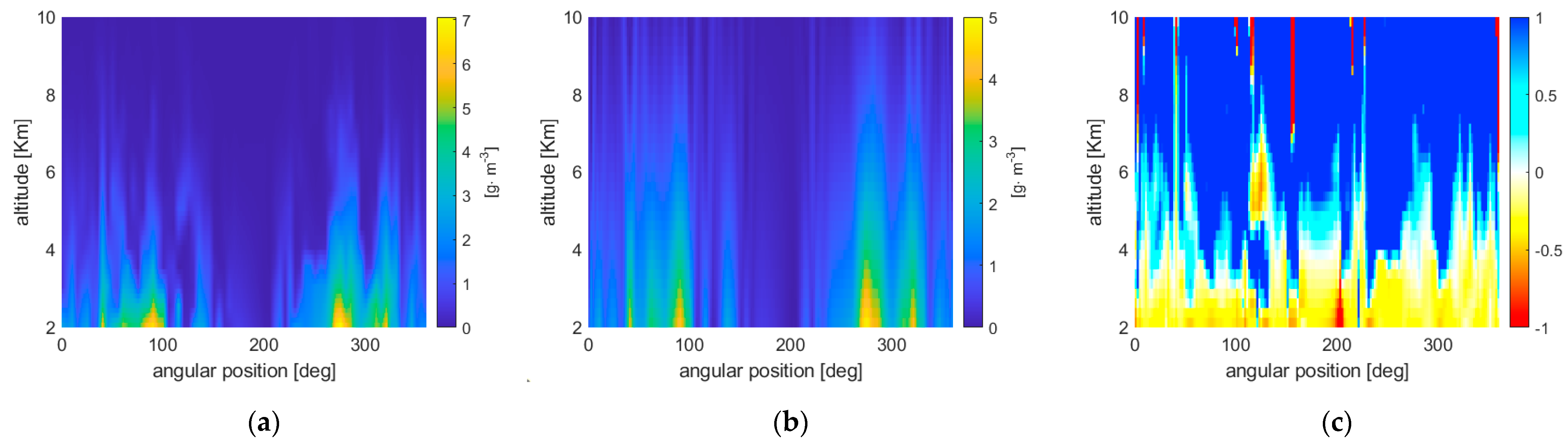
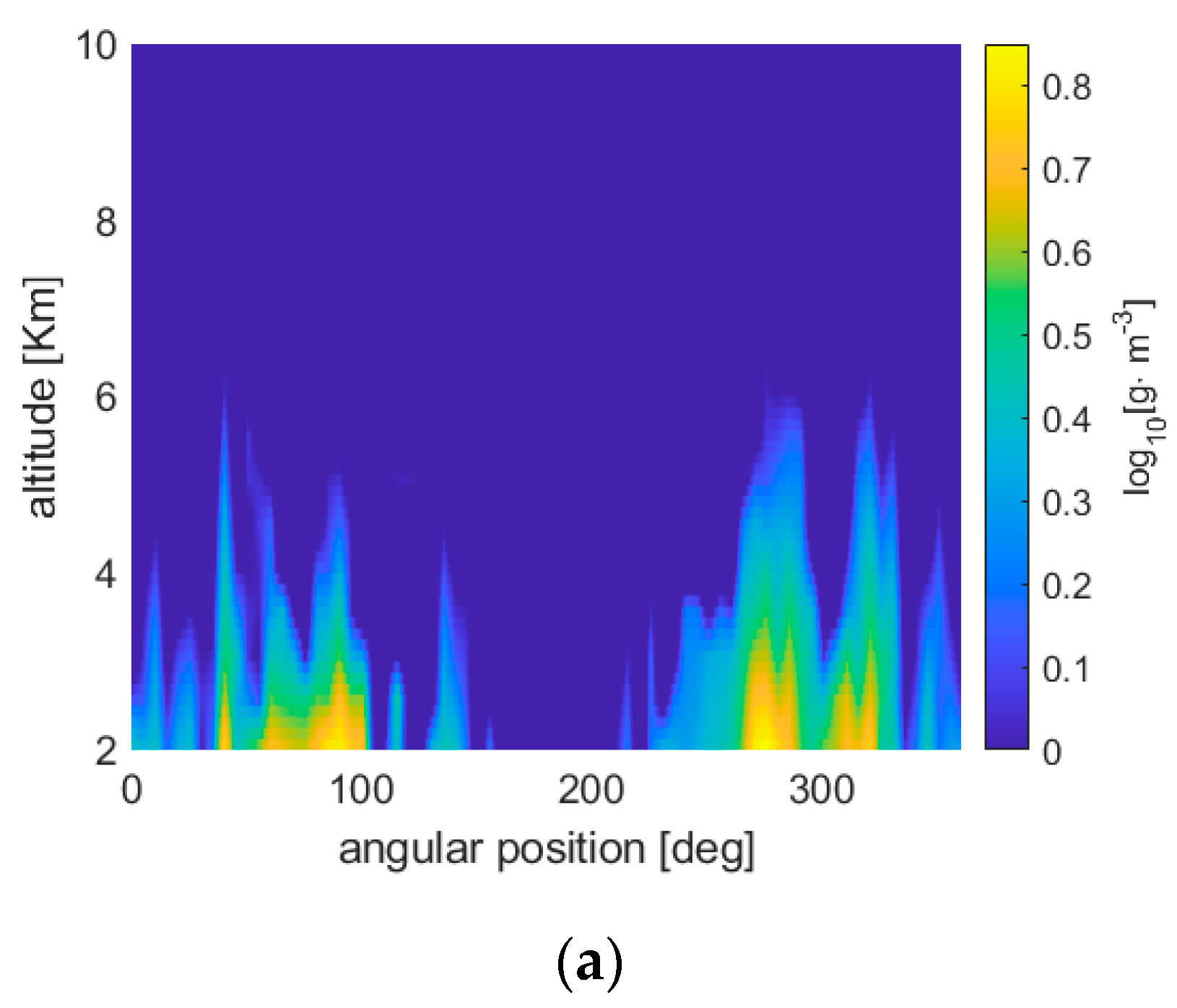
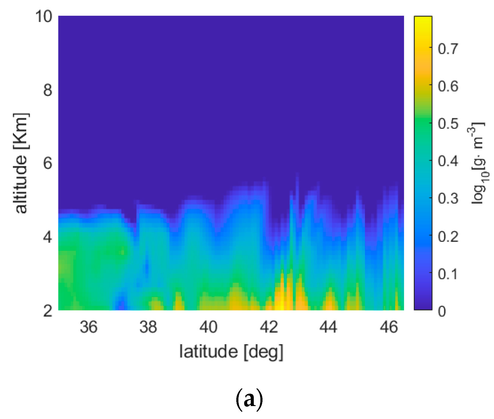
20], i.e., the ECMWF, T511 L91 analysis data of 15 January 2011, 00:00 UTC taken at 20° longitude East. The vertical and angular sampling intervals are 125 m and 1°, respectively. The WV concentration field is shown in
Figure 3a, where the field in polar format is actually shown on a rectangular grid with the horizontal axis and the vertical axis referring to the angular position and the altitude, respectively. For our WV retrieval testing purposes, we did not consider the liquid water content present in such scenario.
In our simulation setup, we assumed the following assumptions concerning the acquisition system and satellite constellation geometry:
Spherical Earth with radius equal to 6378 km;
Rectilinear links connecting transmitters and receivers;
Minimum and maximum tangent altitudes equal to 2 and 10 km, respectively, which implies an opening angle (defined as the angle between the minimum and maximum tangent altitude seen from a transmitting satellite) of 0.2457°;
1 Tx satellite and 5, 10 or 15 Rx satellites on the same circular orbit. The directions of the Tx-Rx links are determined by subdividing the opening angle into equal parts. Since the angles are very small, the tangent altitudes of the microwave links in the scanned annular section result almost equally spaced;
Polar orbit with radius equal to 6651 km (i.e., a satellite altitude equal to 273 km);
Constant angular speed with a revolution period of 90 min;
Integration time at the receiver equal to Ts = 1 s.
The simplifying assumptions (i.e., the hypotheses of spherical Earth, circular orbit and rectilinear propagation of the electromagnetic waves) have been made since the focus of this paper is a compared performance analysis of tomographic algorithms.
In conclusion, under these assumptions, every Ts seconds we have a set of 5, 10 or 15 simultaneous measurements of IWV (one from each Rx satellite).
In the practical ERTA realization, we truncated the infinite summations involved in the function’s decomposition. More specifically, with reference to Equations (4) and (5), n ranges from −Na to Na for what concerns the angular (Fourier) decomposition, while as regards Equations (14) and (16) l ranges from 0 to Nr for the radial decomposition. In our implementation, Na=180 and Nr=41.
Figure 3b,c, respectively, show the ERTA reconstruction and the normalized error between the retrieved WV field and the original one of
Figure 3a. These results refer to a constellation of 6 satellites (1Tx-5Rx). The reconstruction sampling grid has a spacing of 1° and 250 m in the angular and radial directions, respectively. For the generic position (
i,
j), where
i and
j indicate the indices of the discretized angular and radial positions, the normalized error is defined as
where
denotes the reconstruction in (
i,
j) obtained from the inversion of the IWV. Note that high relative errors at the top are encountered due to the significantly low values of WV at the highest altitudes. Based on this first example, it can be stated that ERTA succeeds in retrieving the pattern of the unknown WV map, even though with a clear tendency to underestimating the actual WV content.
5. Results
In this section, we show some reconstruction examples obtained by applying the ERTA and LSATR methods. Unlike the example shown in the previous section, in this case a more realistic scenario is considered by introducing thermal noise at the receiver as well as the phenomenon of scintillation. Such impairments are described in [
20]. For the simulations carried out in this work, we used the same values of the parameters as those utilized in that paper, listed below for the sake of convenience:
Transmitted power: 3 dBW on each NDSA tone;
Frequency channels for NDSA measurement: 17, 19, and 21 GHz, with spectral separation Δf = 0.2 GHz. The channels are selected according to the tangent altitude of the link: the altitude intervals for 17, 19, and 21 GHz are 0–3.5, 3.5–8, and 8–10 km, respectively, for the reasons given in [
16];
Transmit and receive antenna gains: 26.4 dB;
Scintillation: the log-amplitude standard deviation was set to σχ = 0.3 and the zero-lag correlation between the two NDSA frequencies to ρ = 0.85, whereas for the time correlation, dictated by the scintillation bandwidth, we used Bχ = 0.1 Hz.
Thermal noise: the variance of the zero-mean additive white Gaussian noise process is kTeq/Ts, where k is the Boltzmann constant and Teq is the equivalent noise temperature at the receiver, which was set to 25.3 dBK.
Before introducing the simulation results, it is opportune to highlight some of the differences between ERTA and LSATR.
As shown in [
20], LSATR retrieves the WV field as the solution of a linear system, in which the unknowns are the function (i.e., WV concentration) values on the sampling grid chosen for the reconstruction map and the number of equations corresponds to the number of IWV measurements. In general, the Tikhonov regularization term induces a smooth solution, which is driven by a parameter λ to balance smoothness and reconstruction error and whose choice is discussed in [
20]. Another advantage of introducing the regularization term is the fact that in the case of an underdetermined problem (i.e., when the number of unknowns is higher than that of the measurements), a unique solution can be achieved.
In the case of ERTA, it is always possible to retrieve the WV field, but it is not obtained as the solution of a system. In fact, ERTA is based on the expansion by means of a set of orthonormal functions whose coefficients are derived through projections of the function to be decomposed onto the space generated by the orthonormal functions themselves.
As mentioned in the previous section, in the simulations we used three different constellations of satellites (1Tx-5Rx; 1Tx-10Rx; 1Tx-15Rx). This allows us to highlight the behavior of the two retrieval methods as well as the performance of LSATR in both the underdetermined and overdetermined cases.
In the following, we present both a qualitative and a quantitative assessment of the retrieval obtained by using the two inversion algorithms. For this purpose, we show first the ‘true’ and reconstructed maps obtained with ERTA and LSATR, jointly with the local relative error map (i.e., the normalized error field as defined in Equation (17)). After that, we provide a nonlocal quantitative metric of the error by using the percent Normalized Root Mean Square Error (NRMSE) between the ‘true’ and reconstructed WV maps defined as
For the sake of conciseness, the figures show the retrievals referring to only one of the tested satellite constellations, whereas the NRMSE are reported for all of them.
The first simulation outcome we present refers to the same ‘global’ atmospheric scenario considered in the previous section. The reconstruction sampling grid coincides with that used in the previous section (1° × 250 m). Such sampling implies that, in the LSATR case, all three satellite constellations produce an overdetermined inversion problem.
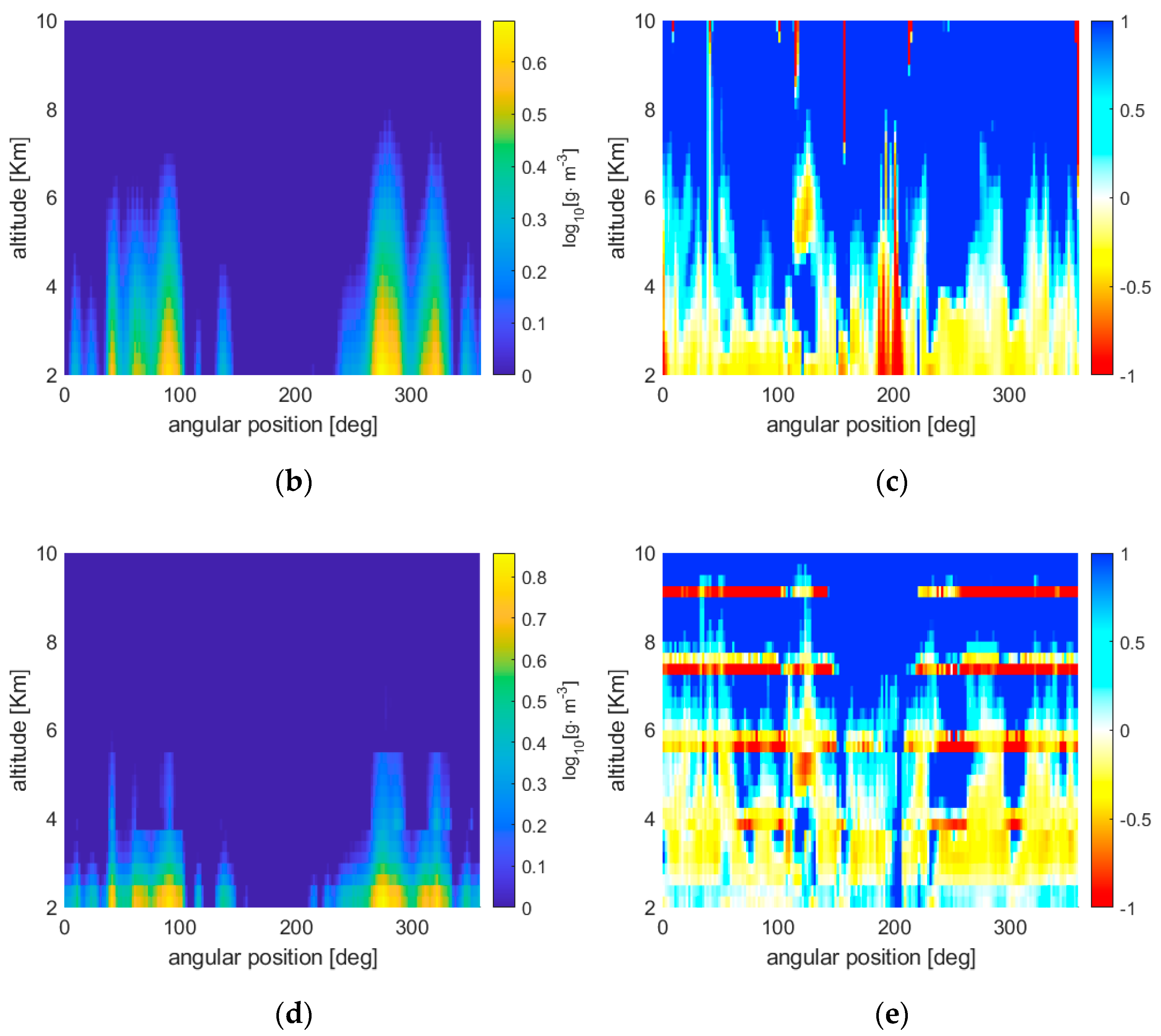
Figure 4 presents the reconstructions and the relative errors obtained by applying the ERTA and LSATR approaches for the 1Tx-5Rx configuration.
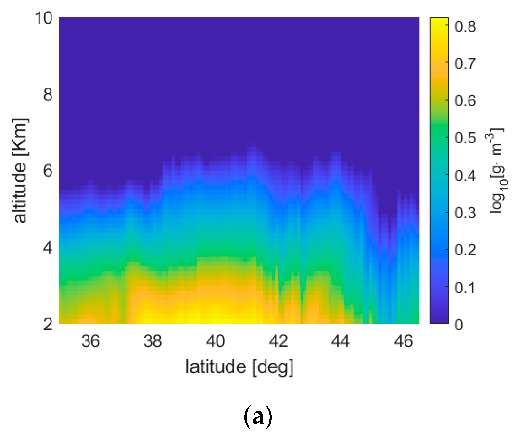
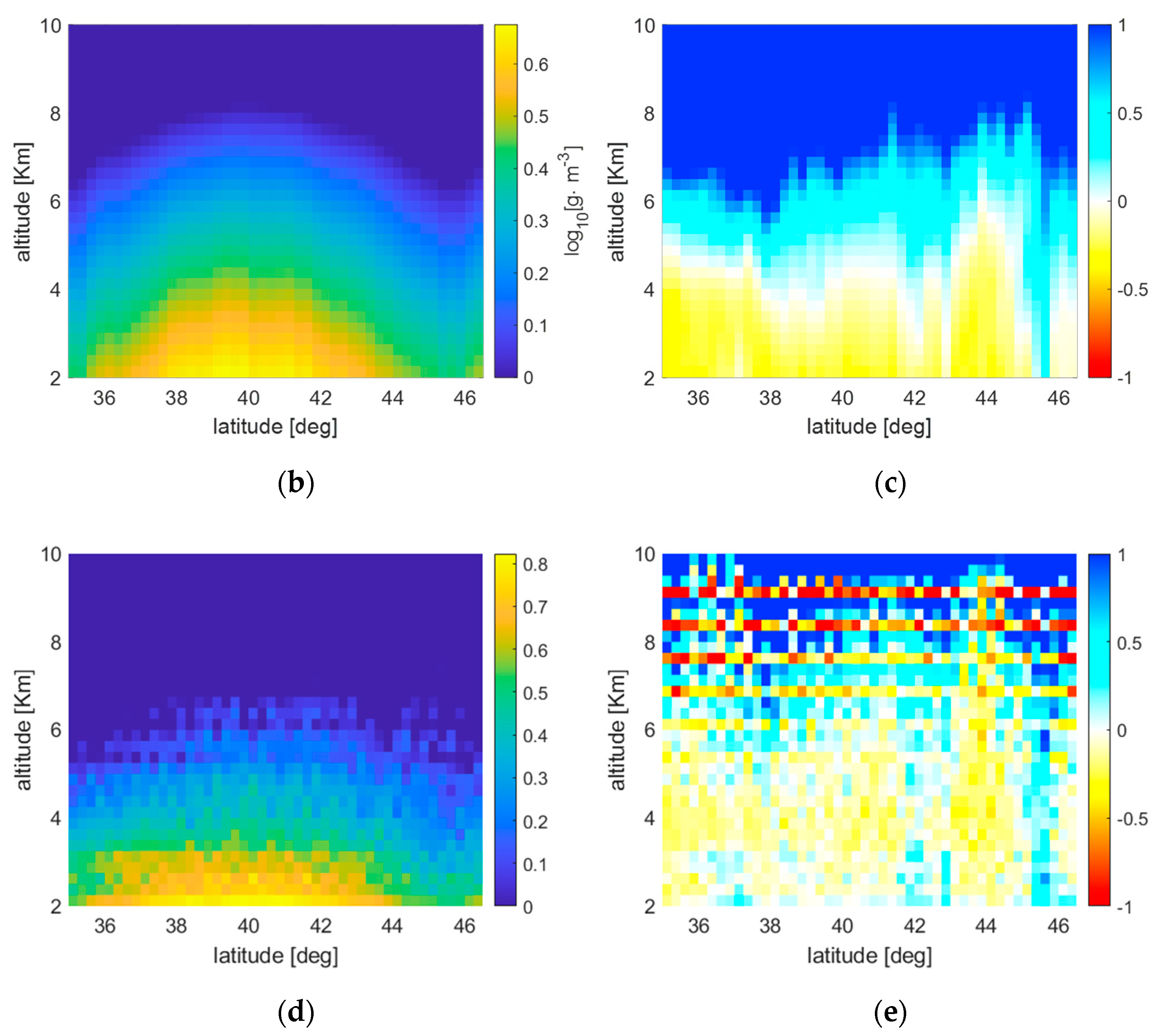
The following
Figure 5,
Figure 6 and
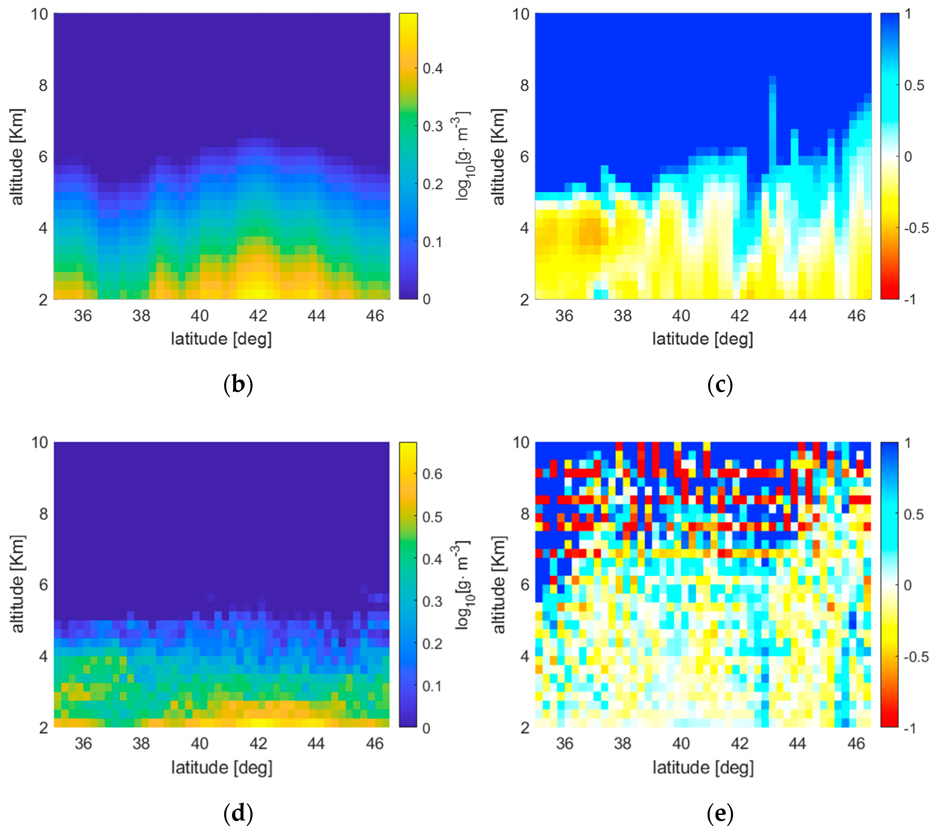
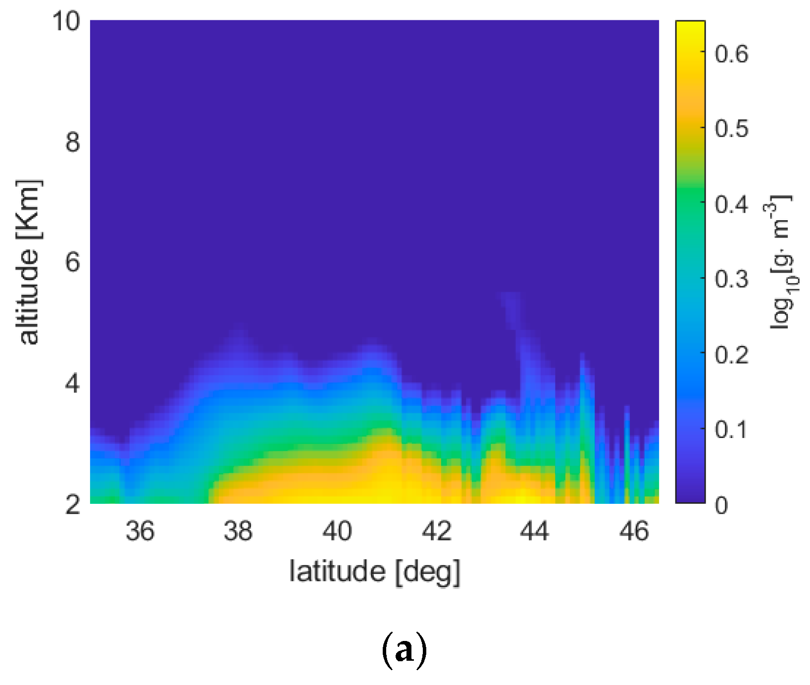
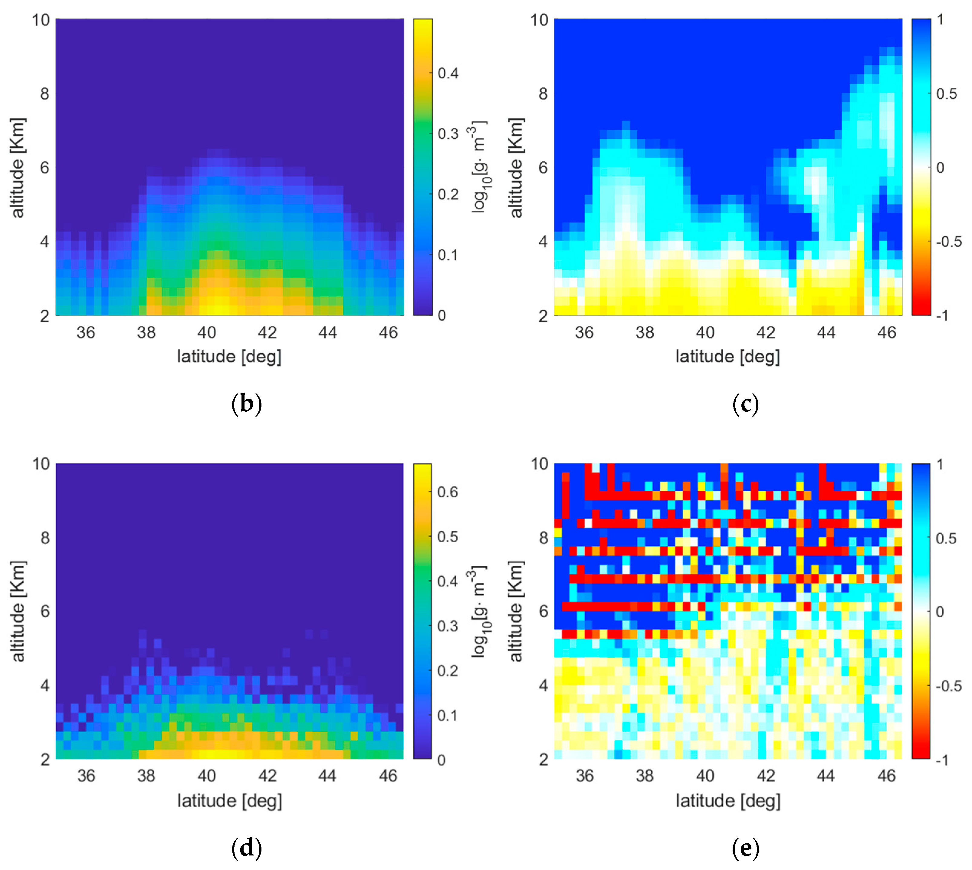
Figure 7, instead, refer to the ERTA and LSATR results obtained using as ‘true’ maps some high resolution WV fields obtained from atmospheric scenarios generated over Tuscany, Italy, through the WRF numerical weather prediction model, initialized with the IFS model of the ECMWF (only the 1Tx-10Rx constellation case is presented in the figures). The sampling grid of the original maps has an angular and radial spacing of 0.1° and 125 m, respectively, whereas the sampling grid of the reconstructed maps has an angular and radial spacing of 0.25° and 250 m, respectively. Such reconstruction map sampling implies that, in the LSATR case, the 1Tx-5Rx configuration produces an underdetermined inversion problem (in the absence of the Tikhonov regularizer), while the other two satellite configurations generate overdetermined inversion problems. The horizontal axis of the figures reports the latitude, as it was assumed that the orbit is coplanar with a meridian. The WV fields refer to three different atmospheric scenarios corresponding to three different dates of 2020. As in the ideal case shown in
Section 4, the liquid water content component of such scenarios was not accounted for.
Observing the retrieval results, it is apparent that the two methods produce error maps with very different spatial behavior. In fact, ERTA exhibits a spatially regular trend while LSATR is characterized by ‘bumps’ in correspondence of the tangent altitudes of the satellite links. The reason for this behavior lies in the quadratic minimization at the base of LSATR, which tends to force to zero the error in the measurement points (the tangent altitudes). As a matter of fact, such bumps could be attenuated by increasing the amount of the regularization term with respect to the ‘fidelity’ term in the Tikhonov unconstrained minimization, but this would produce poorer reconstructions. The balance between the regularization and fidelity terms is driven by the aforementioned parameter λ (chosen as suggested in [
20]). On the contrary, ERTA inherently produces a quite smooth result in the overall reconstruction area.
Notice also that the behavior of the error vs. the altitude is different for the two methods. In fact, at the lowest altitudes the reconstruction error produced by ERTA is lower than that produced by LSATR, while above a certain altitude, depending on the WV field, ERTA constantly overestimates. A reasonable explanation of this behavior of ERTA can be ascribed to the fact that the reconstruction depends on the basis functions used to represent the Radon transform and, successively, to reconstruct the WV field. Such functions are quite regular and, in general, exhibit a decay that is slower than the WV field variations. As a consequence, in the attempt to minimize the approximation error, the retrieved WV field comes out to be a monotonically decreasing function, but with a lower gradient with respect to the ‘true’ WV field. This produces an underestimate of the WV field at the low altitudes.
Quantitative results averaged over spatial areas are reported in
Table 1, which shows the NRMSE for three different altitude ranges (the first two corresponding to the low and high troposphere and the third one to the whole interval considered) and for the three satellite constellations considered. The results are tabulated for the three considered high resolution atmospheric scenarios and for both ERTA and LSATR.
Analyzing
Table 1, several observations can be made. The most evident outcome concerns the behavior of the two inversion algorithms with respect to the number of satellites of the constellation. In the case of LSATR, the performance improves (in some cases significantly) when such number increases: this occurs at the low and high tropospheric intervals and, consequently, over the whole altitude range (2–10 km). As to ERTA, instead, the performance is not influenced by the size of the constellation. This occurs because the elements of the basis of the radial expansion of ERTA do not exhibit a sufficiently rapid decay with altitude, so that the characterization of the radial profiles does not benefit from a higher density of the vertical measurements.
Another element emerging from
Table 1 is that LSATR performs almost always better than ERTA, in particular in the higher tropospheric layer (5–10 km). On the other hand, ERTA appears to be convenient in the lower tropospheric layer (2–5 km) and when the number of satellites is smaller. We can also observe that in the higher altitude range, the percent errors may become quite high, with the performance of ERTA definitely inferior to that of LSATR. Such high NRMSE levels are due to the fact that the average concentration of WV—the denominator in (18)—is much lower in the higher altitude range so that even small absolute errors induce quite high relative errors. However, as mentioned, the number of satellites helps LSATR in improving the performance, but this does not hold for ERTA.
6. Conclusions
The estimation of the atmospheric WV is of extreme interest for the scientific community involved both in meteorological and climatological studies. In particular, the knowledge of the distribution of WV in the troposphere (and specifically, in the low troposphere, where the 95% of the atmospheric WV is concentrated) is of major importance for understanding the dynamics of the meteorological processes. Even though the direct measurements made by radiosondes provide the vertical profiles of WV with good reliability, remote sensing acquisition systems devoted to the estimation of WV on a global scale are of great interest, for instance, for assimilation in numerical weather prediction models. Retrieving the 2D distribution of WV over planes perpendicular to the Earth surface would allow the horizontal structure of the WV fields, which is known in less detail, to be achieved in addition to the vertical profiles.
In this paper, we have reported part of the results of the SATCROSS project, funded by ASI, inherent to a novel approach to retrieve 2D fields of WV concentration by means of a constellation of co-rotating LEO satellites and by using the NDSA method for estimating the IWV along the radio links connecting the satellites. The novel approach is based on the External Reconstruction Tomographic Algorithm, which enables one to retrieve a function, defined on an annular region, from a sampling of its Radon transform, defined in the same region. In our case, the function to be retrieved is the WV concentration and its Radon transform samples are represented by the IWV measurements.
The ERTA approach has been tested by using a simulator that takes into account realistic impairments as well as synthetic atmospheric scenarios, which allow the reconstruction error to be evaluated. The results have been compared to those obtained with another method developed by the authors, based on a least squares algorithm with Tikhonov regularization (LSATR).
In the simulations, we considered constellations with a different number of LEO satellites. The outcomes of the simulations highlight a quite different distribution of the retrieval error between ERTA and LSATR. A quantitative analysis has been made by computing the NRMSE for different altitude ranges corresponding to the low and high troposphere. From both the qualitive and quantitative standpoint, ERTA produces better results at low altitudes and when the number of satellites is smaller; furthermore, its performance seems be poorly affected by the size of the constellation. On the other hand, LSATR exhibits better performance when the number of satellites increases, both in the low and high tropospheric layers.


