An In-Orbit Stereo Navigation Camera Self-Calibration Method for Planetary Rovers with Multiple Constraints

Abstract

In order to complete the high-precision calibration of the planetary rover navigation camera using limited initial data in-orbit, we proposed a joint adjustment model with additional multiple constraints. Specifically, a base model was first established based on the bundle adjustment model, second-order radial and tangential distortion parameters. Then, combining the constraints of collinearity, coplanarity, known distance and relative pose invariance, a joint adjustment model was constructed to realize the in orbit self-calibration of the navigation camera. Given the problem of directionality in line extraction of the solar panel due to large differences in the gradient amplitude, an adaptive brightness-weighted line extraction method was proposed. Lastly, the Levenberg-Marquardt algorithm for nonlinear least squares was used to obtain the optimal results. To verify the proposed method, field experiments and in-orbit experiments were carried out. The results suggested that the proposed method was more accurate than the self-calibration bundle adjustment method, CAHVOR method (a camera model used in machine vision for three-dimensional measurements), and vanishing points method. The average error for the flag of China and the optical solar reflector was only 1 mm and 0.7 mm, respectively. In addition, the proposed method has been implemented in China’s deep space exploration missions.

1. Introduction

With the continuous development of aerospace technologies, many countries have carried out extensive exploration of extraterrestrial bodies, such as to the moon and Mars [1,2,3]. To successfully conduct these tasks, such as planetary rover navigation, high-precision mapping of the detection area, the determination of interior orientation (IO) elements, exterior orientation (EO) elements, and distortion parameters of the cameras are of great significance [4,5]. Because of the influences of environmental factors, such as temperature and pressure, and engine vibration during landing, the camera parameters can be inevitable changed. In 2004, China officially launched the lunar exploration project and named it the “Chang’e Project”. Chang’e-3 is a lunar probe launched in the second phase of China’s lunar exploration project. It consists of a lander and a patrol (“Yutu” lunar rover). The “Yutu” rover patrolled the lunar surface at a speed of 200 m per hour and a rhythm of about 7 m per “step”, and carried out various scientific exploration tasks, including lunar surface morphology and geological structure, lunar surface material composition, available resources, earth plasma layer, etc. The planetary rover is equipped with a pair of stereo navigation cameras for navigation and positioning [3]. Taking Chang’e-3 as an example, the landing process can be divided into the main deceleration stage (15 km), the approaching stage (2 km), the hovering stage (100 m), the obstacle avoidance stage (100 m–30 m), the slow-falling stage (30 m–3 m), and the free-falling stage (<3 m). The vibrations during near-orbit braking, hovering, landing, and particularly free falling can change various parameters of the camera to varying degrees. Therefore, the in-orbit stereo camera self-calibration of planetary rovers is an important study object.

In laboratory conditions, the stereo camera can be calibrated through various high-precision control points, calibration plates, etc. However, when it is in orbit, it is challenging to obtain enough control points or use high-precision calibration plates. Therefore, various information in-orbit must be used as constraints to calibrate the stereo camera. Taking China’s Chang’e-3 as an example, after the planetary rover exits the lander, the camera takes images of the lander for calibration, since the positions and dimensions of multiple components on the lander are rigorously designed and measured in the laboratory. In addition, the solar panel parallel features of the planetary rover can also be used as constraints for the in-orbit self-calibration of stereo cameras. Existing camera calibration methods are designed under laboratory conditions, and the in-orbit self-calibration of stereo cameras remains challenging to complete based on the aforementioned various constraints.

Many studies have been carried out regarding camera calibration. In the early stage, the calibration of traditional monocular cameras is mainly based on the direct linear transformation (DLT) method proposed by Karara and Abdal-Aziz, in which the DLT is performed on pixel coordinates of target points and their spatial coordinates to solve the transformation parameters. Since lens distortion is not considered in the DLT, the calibration accuracy is not ideal [6]. Tsai et al. proposed the radial alignment constraint (RAC) algorithm in 1986 based on DLT. Specifically, after introducing the radial distortion factor and combining it with the linear transformation of the perspective matrix, the calibration parameters can be calculated. The accuracy of the RAC method is improved to a certain extent. However, since it only considers the first-order radial distortion parameters, the efficiency of this method is still limited [7]. Based on the RAC algorithm, Weng et al. improved the distortion model and further improved the applicability of the radial consistency constraint algorithms [8].

To overcome the limitation that the special environment does not meet the calibration requirement and to improve calibration adaptability, Faugeras and Luong proposed the camera self-calibration technology. Specifically, self-calibration is achieved by taking at least two images with a certain degree of overlap and establishing the epipolar transformation relationship to solve the Kruppa equation. However, this method has low accuracy and poor stability, and the Kruppa equation has the singular value problem [9,10]. To solve this problem, Zeller et al. took the sum of the distances from the pixels to the corresponding epipolar line as a constraint and used the Levenberg-Marquardt (LM) algorithm to optimize the equation to obtain the IO elements of the camera. However, the method has the problem of over-parameterization [11]. Jiang et al. and Merras et al. used the epipolar constraint, the LM algorithm, and the genetic algorithm to obtain the optimal solutions for the camera’s IO and EO elements [12,13]. In addition, according to the homography from the calibration plane to the image plane, Zhang et al. solved the IO and the EO separately, which achieved high calibration accuracy. Moreover, because the method has the advantages of easy implementation, high precision, and good robustness, it has been widely adopted by scholars all over the world, which substantially promotes the development of three-dimensional (3D) computer vision from the laboratory to the real world [14].

Regarding the calibration of binocular cameras, Tan et al. first reconstructed the homography transformation relationship between a stereo image pair based on the homologous points extracted from the stereo image pair and then obtained the calibration parameters based on this transformation. This method has the advantages of strong adaptability, flexibility, and high speed but has poor stability and low accuracy [15]. Shi et al. used no less than six non-coplanar 3D lines to perform DLT, carried out linear estimation of the projection matrix, and jointly used a nonlinear optimization algorithm and distortion parameters to perform a combined adjustment. This method is a novel calibration method [16]. Moreover, Caprile et al. proposed the classic vanishing point theory in 1990, that is, two or more parallel lines can converge at one point after infinite extension, and the convergence point is called the vanishing point [17]. Wei et al. introduced the vanishing point theory into camera calibration. Multiperspective images of the target are first taken, and then the convergence point after perspective projection, i.e., the vanishing point, is obtained using the spatial parallel lines in the three orthogonal directions of a cube. Camera self-calibration is realized based on the relationship between the parallel lines and the geometric parameters to be calibrated. Since three parallel lines in orthogonal directions are needed in this method, the scope of application is limited [18]. In addition, Fan et al. proposed a self-calibration method based on the circular point pattern [19]. Zhao et al. used several tangent circles passing the endpoints of the diameter as the calibration target. Since the tangent lines of the circles at the two ends are parallel, the vanishing point is determined, and camera calibration is then carried out based on the image plane coordinates of the circle points [20]. Based on this work, Peng et al. proposed a plane transformation-based calibration method. By fitting the pixel coordinates of the actual circle center, Zhang’s method is used for camera calibration and achieves a high calibration accuracy [21]. To date, most studies have focused on the establishment of bundle adjustment models for camera calibration. Brown et al. first applied bundle adjustment to camera calibration by constructing a mathematical model combining the perspective projection model and distortion model, which enabled the use of nonmetric cameras for photogrammetry [22]. Huang et al. Proposed the fusion beam method and high-precision global navigation satellite system (GNSS) to self-calibration. However, GNSS cannot be used in deep space exploration [23]. Deng et al. used the LM algorithm to optimize the calibration results based on the relative position between the binocular stereo cameras. Moreover, Zheng et al. and Xie et al. further optimized the model based on indicators such as the unit weight root-mean-square error (RMSE) to improve the calibration accuracy and obtain good calibration parameters [24,25]. Subsequently, Liu et al. applied the bundle adjustment method to the positioning of planetary rovers, and it has a certain application value [26].

The first studies on the stereo camera calibration of planetary rovers were from Bell and Mahboub et al. Specifically, based on the high-precision calibration points on the Curiosity Rover and the central attitude horizontal-vertical (CAHV) model [27], the in-orbit stereo camera calibration of the Curiosity Rover was achieved [28,29]. Gennery et al. introduced the radial distortion parameter to the CAHV model and proposed the CAHVOR model (C is the vector from the origin of the ground coordinate system to the photography center, A is the unit vector perpendicular to the image plane, H and V are the horizontal vector and the vertical vector respectively, and the three are orthogonal to each other. O is the unit vector of the optical axis. When the image plane is not perpendicular to the optical axis, O is used to describe the direction of the optical axis, when the two are perpendicular, A and O coincide. R is the radial distortion parameter in the ground coordinate system.) [30], which has been applied in the camera calibration of the Opportunity and Courage Rovers.. The teleoperation system of planetary rovers in China’s deep space exploration missions mostly uses photogrammetric mathematical models, and the conversion relationship between the mathematical models and the CAHVOR models is very complex. In addition, China’s planetary rovers are not equipped with high-precision calibration points. Therefore, the above methods cannot be directly applied for the in-orbit camera calibration of China’s planetary rovers. According to the geometric characteristics of the planetary rover itself and the carried objects, Workman et al. took the fixed geometric relationships among the planetary rover, the sun, and the horizon as constraints for camera self-calibration, but the improvement in calibration accuracy was limited [31]. Wang et al. used the rotation angle between the stereo cameras as the constraint for camera calibration [32], yet the in-orbit test has not been conducted.

In summary, although the above methods have achieved promising results, the in-orbit stereo camera calibration in the deep space exploration missions needs to be implemented in accordance with the actual conditions of each country. Because of limited available features on the planetary surface and possible high light intensity, a target-based calibration scheme is difficult to implement, and thus, self-calibration technology needs to be developed. This study proposed a self-calibration bundle adjustment method with multiple feature constraints for in-orbit camera calibration. We summarize our contributions as follows:

(1) A combined self-calibration bundle adjustment method with multiple feature constraints is constructed, which makes full use of the limited conditions in orbit, can complete the calibration under the condition of a small amount of observation data, and effectively improves the calibration accuracy in-orbit.

(2) An adaptive intensity weighted line extraction method is proposed, which ensures the completeness of line detection in different directions and effectively improves the extraction effect.

(3) The redundant observations with different constraints are analyzed, and the relationship between the redundant observations and the standard deviation of the model adjustment result is obtained, which provides a reference for the optimization of other bundle adjustment models.

(4) The proposed method can provide a reference for in-orbit camera calibration of planetary rovers in the deep space exploration missions of all countries.

The remaining sections of this paper are as follows: Section 2 describes the overall process and each part of the proposed method. Section 3 presents a series of experiments on different experimental conditions, and the results are compared. Section 4 provides the conclusions.

2. Methods

2.1. Stereo Vision System and Coordinate Systems of Planetary Rovers

This section describes the structure of the planetary rover’s stereo vision system and the parameters of each component, and then different coordinate systems and their transformation relationship are explained.

2.1.1. Navcam System of Planetary Rovers

Currently, the Navcam system is one of the key components for navigation and positioning of planetary rovers. Taking China’s Chang’e-3 rover as an example, its Navcam system is composed of a pair of navigation cameras, a pair of panoramic cameras, a pair of obstacle avoidance cameras, a mast system and an inertial measurement unit (IMU), as shown in Figure 1. The navigation cameras use fixed-focus lenses with a medium focal length and are installed on the camera gimbal, which is fixed to the top of the planetary rover through the mast system. The height of the navigation cameras is approximately 1500 mm above the ground [32]. The cameras can rotate 360° in the horizontal plane, and −70° to +80° around the pitch axis. The mast system consists of three joints to enable roll, yaw, and pitch movement of the navigation cameras and the panoramic cameras [33]. In the remote-control mode, the planetary rover maps the surrounding landscape within 120° after moving a fixed distance, and the data are sent back to the ground to generate a digital orthophoto map (DOM), digital elevation model (DEM), and other cartographic products for path planning for the next navigation point [34].

2.1.2. Posture Model of the Stereo Navigation Camera

The navigation cameras on the Chang’e-3 rover are parallel binocular stereo cameras and can be considered pinhole imaging cameras, where the two main optical axes are parallel to each other, the horizontal axes are collinear, and cameras are placed with a certain baseline length, as shown in Figure 2. B_lr is the photogrammetric baseline vector, and the length is the distance between the optical centers of the left and right cameras.

Assume that the rotation matrices between the image coordinate systems of the left and right cameras and the ground coordinate system of the control points are ${\mathrm{R}}_l$ and ${\mathrm{R}}_r$. The center of the left and right images are ${\mathrm{S}}_l$ and ${\mathrm{S}}_r$. Taking the image coordinate system of the right camera as a reference, then, the relative rotation of the left camera is ${\mathrm{R}}_{lr}$. Based on the baseline vector between the left and right navigation cameras, the transformation relationship between the rotation matrices of the stereo navigation cameras is

$${\mathrm{R}}_r={\mathrm{R}}_l{\mathrm{R}}_{lr}$$

(1)

According to Equation (1), the transformation relationship between the EO elements can be obtained:

$${\mathrm{S}}_r-{\mathrm{S}}_l={\mathrm{R}}_{lr}{\mathrm{T}}_{lr}={\mathrm{R}}_l^T{\mathrm{R}}_r{\mathrm{T}}_{lr}$$

(2)

2.2. Bundle Adjustment Model for Binocular Cameras

The bundle adjustment model is a classic high-precision adjustment model used in the field of photogrammetry. In this study, the bundle adjustment model was used as the basic model for combined adjustment [35]. According to the definitions of the image plane coordinate system and the photogrammetric coordinate system, the classic collinear equation can be established using the stereo navigation images:

$$\{\begin{array}{l}x+x_0+\Delta x=-f\frac{a1(X-X_S^{})+b1(Y-Y_S^{})+c1(Z-Z_S^{})}{a3(X-X_S^{})+b3(Y-Y_S^{})+c3(Z-Z_S^{})}\\ y+y_0+\Delta y=-f\frac{a2(X-X_S^{})+b2(Y-Y_S^{})+c2(Z-Z_S^{})}{a3(X-X_S^{})+b3(Y-Y_S^{})+c3(Z-Z_S^{})}\end{array}$$

(3)

where $(x,y)$ are the coordinates of an image point in the image plane, $(X,Y,Z)$ are the corresponding coordinates under the photogrammetric coordinate system, $(X_S,Y_S,Z_S)$ are the translation components of the EO elements, and (a1, b1, c1), …, (a3, b3, c3) are the elements of the rotation matrix R. $(x_0,y_0)$ are the IO elements, and $(\Delta x,\Delta y)$ are the coordinate differences of image points in the left and right cameras:

$$\{\begin{array}{l}\Delta x=(x-x_0)(k_1{r}^2+k_2{r}^4)+(x-x_0)+p_2(r^2+2{(x-x_0)}^2)+2p_1(x-x_0)(y-y_0)\\ \Delta y=(y-y_0)(k_1{r}^2+k_2{r}^4)+(y-y_0)+p_1(r^2+2{(y-y_0)}^2)+2p_2(x-x_0)(y-y_0)\\ r=\sqrt{{(x-x_0)}^2+{(y-y_0)}^2}\end{array}$$

(4)

where $k_1,k_2$ are the first-order and second-order radial distortion parameters, respectively, and $p_1,p_2$ are the first-order and second-order tangential distortion parameters, respectively.

Through a Taylor series expansion of Equation (4), the linearized bundle adjustment error model for the binocular camera is obtained:

$$\mathrm{V}=\mathrm{A}{\mathrm{t}}_1+\mathrm{B}{\mathrm{t}}_2+\mathrm{C}{\mathrm{X}}_1+\mathrm{D}{\mathrm{X}}_2+\mathrm{F}{\mathrm{X}}_3-\mathrm{L}$$

(5)

where $\mathrm{V}={[v_x,v_y]}^T$ is the correction of the image point residuals, and ${\mathrm{t}}_1={[\Delta X_S^l,\Delta Y_S^l,\Delta Z_S^l,\Delta {\phi }^l,\Delta {\omega }^l,\Delta {\kappa }^l]}^T$ and ${\mathrm{t}}_2={[\Delta X_S^r,\Delta Y_S^r,\Delta Z_S^r,\Delta {\phi }^r,\Delta {\omega }^r,\Delta {\kappa }^r]}^T$ are the corrections of the EO elements in the left and right images, respectively. ${\mathrm{X}}_1={\left[\Delta x_0^l,\Delta y_0^l,\Delta f_{}^l\right]}^T$ and ${\mathrm{X}}_2={\left[\Delta x_0^r,\Delta y_0^r,\Delta f_{}^r\right]}^T$ are the corrections of the IO elements in the left and right images, respectively. ${\mathrm{X}}_3={\left[\Delta X,\Delta Y,\Delta Z\right]}^T$ is the correction of the photogrammetric coordinate system, D and F are the coefficient matrices corresponding to ${\mathrm{X}}_2$ and ${\mathrm{X}}_3$, respectively, $\mathrm{L}={[l_x,l_y]}^T$ is the coordinate vector of the image point, and (A, B, C) is the corresponding coefficient matrix.

2.3. Adaptive Line Extraction and Constraint Model

Lens distortion is one of the key factors in the calibration of navigation cameras. The straight line feature is a typical pattern seen in the image of the solar panel of the lander and the planetary rover, and it is not subject to the influence of vibrations. Thus, using line features as calibration constraints can ensure the robustness of the calibration algorithm and improve the accuracy of calibration parameters. In the current line extraction methods, the overall image is used to determine the threshold. However, the images containing solar panels can be affected by the lunar illumination such that the line features of solar panels in different directions are disrupted, as shown in Figure 3. This disruption can prevent the extraction of lines with poor gradients. Moreover, if manual extraction is used, the extraction result might deviate from the true position of the line. Therefore, an adaptive brightness-weighted line extraction method was proposed.

During extraction, the extracted lines are optimized and straightened based on the extracted edges. Specifically, based on the gradient template shown in Figure 4, the gradient magnitude and direction of the pixels are calculated, and the average gradient direction of the 3 × 3 neighborhood pixels is used to replace the original gradient of the pixel. By traversing the entire image, the gradient magnitude and direction of all pixels are obtained. Figure 5 shows the histograms of gradient directions of four navigation images.

Figure 5 and the statistical results of many experiments show that the distribution of the gradient directions of the rover navigation images in the Chinese lunar exploration project satisfies a Gaussian distribution. Therefore, the images are divided into different gradient intervals according to the confidence interval (CI) of a Gaussian distribution, and the pixel gradient threshold of each interval is determined [36,37,38]. According to the properties of a Gaussian distribution, 99.7% of the area is within the range of three standard deviations (SDs) $3\delta$. The subintervals of the gradient direction distribution are established according to the SD, as shown in Figure 6. In total, there are eight subintervals, i.e., $[<-3\delta ]$, $[-3\delta ,-2\delta ]$, $[-2\delta ,-\delta ]$, $[-\delta ,\mu ]$, $[\mu ,\delta ]$, $[\delta ,2\delta ]$, $[2\delta ,3\delta ]$ and $[>3\delta ]$. The red vertical line is the expected value of the gradient direction of the entire image.

To minimize the influence of illumination on the image gradient, the normalized brightness is used as a basis for weight determination, and the dual thresholds for edge extraction in different regions are also determined. The calculation of the weight and upper threshold is shown in Equation (6), and the lower threshold is 0.4 times the upper threshold. Lastly, edge extraction in the dark part of the image is optimized.

$$\{\begin{array}{l}{P}_i\hspace{0.17em}\hspace{0.17em}\hspace{0.17em}=\hspace{0.17em}\hspace{0.17em}1-L(x,y)\\ T{h}_m=\hspace{0.17em}\hspace{0.17em}{\displaystyle \sum _{i=1}^n\left(T_i·P_i\right)}/{\displaystyle \sum _{i=1}^n{P}_i}\end{array}$$

(6)

where $P_i$ is the weight at $(x,y)$, m is the number of subintervals, $T{h}_m$ is the upper threshold for the m-th interval, and n is the number of pixels in the image.

After obtaining the edge extraction results, the edge pixels are constructed into an edge chain. Specifically, according to the distribution of the gradient directions of the edge chain elements, pixelwise tracking is used to perform the initial straight-line detection. The process is as follows:

(1) A histogram of the gradient directions of the edge pixels is established (Figure 7), and the corresponding seed point is set in each edge chain along the peak gradient direction (Figure 8a).

(2) Starting from the seed point, the pixels on both sides are tracked. If the gradient direction difference in the connection line between the seed point and the pixel is less than the empirical threshold of 22.5° [39], the tracking continues. Otherwise, the tracking is stopped, and a line index is created.

(3) All edge chains in the image are traversed for line detection. The edge growth process is shown in Figure 8.

To obtain continuous straight lines, the detected line chains need to be processed via connection and fitting. First, the obtained initial straight lines are linearly fitted to obtain the slope. Then, the initial straight lines are connected based on the constraints, such as the distance between straight lines and the consistency between the slope of the line connecting the two centers of gravity (CG). Lastly, length inspection is performed to obtain the final straight lines.

(1) Fitting and connection of initial straight lines. Based on the principle of least squares, the slope $\widehat{a}$ of the lines is calculated using Equation (7).

$$\widehat{a}=\frac{{\displaystyle \sum _{i=1}^n\left(x_i-\overline{x}\right)\left(y_i-\overline{y}\right)}}{{\displaystyle \sum _{i=1}^n{\left(x_i-\overline{x}\right)}^2}}=\frac{{\displaystyle \sum _{i=1}^n{x}_i{y}_i-n\overline{x}\overline{y}}}{{\displaystyle \sum _{i=1}^n{x}_i{}^2-n{\overline{x}}^2}}$$

(7)

where n is the number of elements in the line, ($x_i,y_i$) are the pixel coordinates, and ($\overline{x},\overline{y}$) are the coordinates of the CG of the line. Then, the direction of the line is calculated based on the slope. To increase the calculation speed, the direction difference between the lines is taken as the initial criterion for line connection. If the direction difference between two lines is less than 22.5°, they can be considered the same line. Otherwise, they are not the same line.

Assume that the initial line chain includes the yellow elements in Figure 9, and the line chain to be connected includes the blue elements. After connecting the center of the two chains, if the distance between every pixel on the chain and the CG line is less than one pixel, then the two lines can be connected. In addition, the blank pixels between the two lines are evaluated. If the gradient direction difference between these pixels and the two lines is less than 22.5°, then the two lines are considered the same line. Lastly, the line chain to be connected and the blank pixels are merged into the initial line chain. All initial line chains are traversed in this manner until all connections are completed.

(2) Deletion of short line chains. Based on the Helmholtz principle, the number of false alarms (NFA) is introduced [39]. Assuming that A is a line chain with a length of l, in an $N\times N$ image, at least k pixels are on the line chain. Then, the NFA is defined as

$$NFA\left(l,k\right)=N^4·{\displaystyle \sum _{i=k}^l{p}^i}{\left(1-p\right)}^{l-i}$$

(8)

where $N^4$ is the total number of all possible line chains, and $p$ is the direction accuracy of a line. Since the threshold used above is 22.5°, p = 0.125. If $NFA\left(l,k\right)>1$, the probability that the line belongs to the background is high, and it can be considered a false line. If $NFA\left(l,k\right)\le 1$, the probability that the line belongs to the foreground is high, and it can be considered a straight line with high robustness.

When $NFA\left(l,k\right)\le 1$ and the length is the shortest, k = l, i.e., $NFA\left(l,l\right)=N^4\ast p^l\le 1$. Then, the following inequality can be obtained:

$$l\ge \frac{-4\log \left(N\right)}{\log \left(p\right)}$$

(9)

Then, the minimal line length $L_{\min }$ is obtained through Equation (9). If the length of an initial line is greater than $L_{\min }$, the line is retained; otherwise the line is discarded. After all the lines are checked for length, the final line extraction result is obtained.

The feature lines on the solar panels of the lander and the rover were extracted using the method above. Then, based on the collinear nature of the points on a line, the lines can be used as an adjustment constraint to improve the calibration accuracy. Assuming that the points $N_i(X_i,Y_i,Z_i)$, $N_1(X_1,Y_1,Z_1)$ and $N_2(X_2,Y_2,Z_2)$ are on the same line, the ground coordinates of these three points should satisfy the requirement that the slope of the line connecting any two points is the same:

$$\frac{X_i-X_1}{X_2-X_1}=\frac{Y_i-Y_1}{Y_2-Y_1}=\frac{Z_i-Z_1}{Z_2-Z_1}$$

(10)

where $(X_i,Y_i,Z_i)$ represent the three-dimensional coordinates of the i-th point on a certain line, $(X_1,Y_1,Z_1)$ and $(X_2,Y_2,Z_2)$ represent the three-dimensional coordinates of the start and end points of the line, respectively.

The error model of collinear constraint was constructed according to Equation (10):

$${\mathrm{G}}_1{\mathrm{X}}_3-{\mathrm{L}}_1=0$$

(11)

where ${\mathrm{X}}_3$ is the correction of a point in the photogrammetric coordinate system, ${\mathrm{G}}_1$ is the corresponding coefficient matrix, and L₁ is the residual matrix. When using collinear conditions to construct an adjustment model, we do not use all points on the line to achieve constraints, but only use the starting point, midpoint and end point.

2.4. Models of Distance Constraint, Coplanar Constraint and Relative Pose Constraint

In the traditional bundle adjustment model, the control points and the pixel coordinates are considered observations, which lead to many unknowns and requires more control points or more images, thus causing the rank reduction in the coefficient matrix of the normal equation [40]. Therefore, this study jointly used non-photogrammetric and photogrammetric observations or conditions to carry out the adjustment. In addition to the line feature constraints described in Section 2.3, the other non-photogrammetric observations used as feature constraints include the following three types:

(1) Distance constraint. In the calibration of the Chang’e-3 planetary rover’s navigation cameras, a high-precision total station measurement system can be used to accurately measure the corners of the national flag and the solar panels and other feature points, which are then used as the virtual control points for in-orbit calibration. Since the dimensions of the flag and solar panels do not change with vibration, the distances between these virtual control points should remain the same as the laboratory measurements. Hence, the distance between two points can be used as a constraint to improve the calibration accuracy. In addition, according to the adjustment theory, the error equation must have two basic conditions, i.e., a coordinate system and a length reference, while the adjustment based on the collinear equation only has a coordinate reference. Thus, the actual length between the control points should be used in combination with the collinear equation during adjustment [41]. The distance between two virtual control points is calculated in Equation (12):

$$\sqrt{{(X_m-X_n)}^2+{(Y_m-Y_n)}^2+{(Z_m-Z_n)}^2}-D_{mn}=\Delta D_{mn}$$

(12)

where $(X_m,Y_m,Z_m)$ and $(X_n,Y_n,Z_n)$ are the coordinates of the control points in the photogrammetric coordinate system, and $D_{mn}$ is the high-precision laboratory-measured distance between the two control points, and $\Delta D_{mn}$ is the residual between the distance obtained from the observation and the true distance.

The coordinates of the virtual control points are considered virtual observations with errors, and by performing a Taylor series expansion on Equation (12), the linearized error equation can be obtained:

$${\mathrm{V}}_3={\mathrm{F}}_3{\mathrm{X}}_3-{\mathrm{L}}_3$$

(13)

where ${\mathrm{V}}_3$ is the correction of the distance residual, ${\mathrm{X}}_3$ is the correction of the coordinates of the virtual control point, ${\mathrm{F}}_3$ is the corresponding coefficient matrix, and ${\mathrm{L}}_3$ is a constant term obtained by substituting the virtual control point’s coordinates before correction into Equation (12).

(2) Planar conditions. On the solar panels of the lander and the planetary rover are many coplanar feature points. Therefore, based on the coplanar property, the coordinates of virtual control points or connection points can be substituted into the coplanar equation to realize coordinate adjustment, thereby improving the accuracy. Assuming that the points $N_i(X_i,Y_i,Z_i)$, $N_1(X_1,Y_1,Z_1)$, $N_2(X_2,Y_2,Z_2)$, and $N_3(X_3,Y_3,Z_3)$ are on the same plane, the coplanar equation of the four points is as follows:

$$\left|\begin{array}{ccc}{X}_i-X_1& Y_i-Y_1& Z_i-Z_1\\ X_i-X_2& Y_i-Y_2& Z_i-Z_2\\ X_i-X_3& Y_i-Y_3& Z_i-Z_3\end{array}\right|=0$$

(14)

This expression can be rewritten in a function format:

$$\{\begin{array}{l}(X_i-X_1)(Y_2-Y_1)-(X_2-X_1)(Y_i-Y_1)=0\\ (X_i-X_1)(Z_2-Z_1)-(X_2-X_1)(Z_i-Z_1)=0\end{array}$$

(15)

After linearization of Equation (15), the following equation is obtained:

$${\mathrm{G}}_2{\mathrm{X}}_3^{}-{\mathrm{L}}_2^{}=0$$

(16)

where ${\mathrm{X}}_3^{}$ is the correction of the 3D coordinates, ${\mathrm{G}}_2$ is the corresponding coefficient matrix, and ${\mathrm{L}}_2$ is the corresponding residual.

(3) Constraint on the relative position and orientation of the cameras. In every photographic station, the relative position and orientation between the left and right navigation cameras are the same. Assume that two image pairs are used for adjustment, and both satisfy Equations (1) and (2). Then, based on the orthogonal property of the rotation matrix, the following equations can be obtained:

$$\{\begin{array}{l}{({\mathrm{R}}_l^T{\mathrm{R}}_r)}_i-{({\mathrm{R}}_l^T{\mathrm{R}}_r)}_j=0\\ {\left[{\mathrm{R}}_r^T{\mathrm{R}}_l^{}({\mathrm{S}}_r-{\mathrm{S}}_l)\right]}_i-{\left[{\mathrm{R}}_r^T{\mathrm{R}}_l^{}({\mathrm{S}}_r-{\mathrm{S}}_l)\right]}_j=0\end{array}$$

(17)

where the subscripts i and j are the number of the stereo image pair.

After linearization of Equation (17), the error equation of the relative position and orientation constraint of the binocular stereo cameras is obtained:

$${\mathrm{A}}_i^l{\mathrm{t}}_1^i+{\mathrm{B}}_i^r{\mathrm{t}}_2^i-{\mathrm{A}}_j^l{\mathrm{t}}_1^j-{\mathrm{B}}_j^r{\mathrm{t}}_2^j-{\mathrm{L}}_{ij}^{}=0$$

(18)

where $({\mathrm{t}}_1^i,{\mathrm{t}}_2^i,{\mathrm{t}}_1^j,{\mathrm{t}}_2^j)$ represents the left and right EO elements of the i-th and j-th image pair, $({\mathrm{A}}_i^l,{\mathrm{B}}_i^r,{\mathrm{A}}_j^l,{\mathrm{B}}_j^r)$ represents the first-order partial derivative of the EO elements of the i-th and j-th image pair, and ${\mathrm{L}}_{ij}^{}$ is the residual error obtained after substituting the result of the previous iteration.

2.5. Final Calibration Model and Weighting of Observations

More radial and tangential distortion parameters do not necessarily mean a higher accuracy, because too many nonlinear parameters can reduce the robustness of the solution [42]. Therefore, the final calibration parameters used in this study included the IO elements of the left and right cameras $(u_0,v_0,f)$, the radial distortion parameters $k_1,k_2$, and the tangential distortion parameters $p_1,p_2$. To improve the overall accuracy of the solution, the coordinates of the virtual control points and the connection points $(X,Y,Z)$ are considered observations with errors and adjusted. Based on Equation (3), the above parameters, the constraint Equations (11), (13), (16) and (18), and the weight matrix $\mathrm{P}$ of the observations, the final indirect adjustment model with multiple constraints is

$$\{\begin{array}{l}{\mathrm{V}}_1=\mathrm{A}{\mathrm{t}}_1\hspace{0.17em}\hspace{0.17em}\hspace{0.17em}\hspace{0.17em}\hspace{0.17em}\hspace{0.17em}\hspace{0.17em}\hspace{0.17em}+\mathrm{C}{\mathrm{X}}_1\hspace{0.17em}\hspace{0.17em}\hspace{0.17em}\hspace{0.17em}\hspace{0.17em}\hspace{0.17em}\hspace{0.17em}\hspace{0.17em}\hspace{0.17em}\hspace{0.17em}\hspace{0.17em}+{\mathrm{F}}_l{\mathrm{X}}_3-{\mathrm{L}}_l\hspace{0.17em}\hspace{0.17em}\mathrm{P}\\ {\mathrm{V}}_2=\hspace{0.17em}\hspace{0.17em}\hspace{0.17em}\hspace{0.17em}\hspace{0.17em}\hspace{0.17em}\hspace{0.17em}\hspace{0.17em}+\mathrm{B}{\mathrm{t}}_2\hspace{0.17em}\hspace{0.17em}\hspace{0.17em}\hspace{0.17em}\hspace{0.17em}\hspace{0.17em}\hspace{0.17em}\hspace{0.17em}+\mathrm{D}{\mathrm{X}}_2+{\mathrm{F}}_r{\mathrm{X}}_3-{\mathrm{L}}_r\hspace{0.17em}\hspace{0.17em}\mathrm{P}\\ {\mathrm{V}}_3=\hspace{0.17em}\hspace{0.17em}\hspace{0.17em}\hspace{0.17em}\hspace{0.17em}\hspace{0.17em}\hspace{0.17em}\hspace{0.17em}\hspace{0.17em}\hspace{0.17em}\hspace{0.17em}\hspace{0.17em}\hspace{0.17em}\hspace{0.17em}\hspace{0.17em}\hspace{0.17em}\hspace{0.17em}\hspace{0.17em}\hspace{0.17em}\hspace{0.17em}\hspace{0.17em}\hspace{0.17em}\hspace{0.17em}\hspace{0.17em}\hspace{0.17em}\hspace{0.17em}\hspace{0.17em}\hspace{0.17em}\hspace{0.17em}\hspace{0.17em}\hspace{0.17em}\hspace{0.17em}\hspace{0.17em}\hspace{0.17em}\hspace{0.17em}{\mathrm{F}}_3{\mathrm{X}}_3-{\mathrm{L}}_3\hspace{0.17em} \mathrm{P}\\ {\mathrm{G}}_4{\mathrm{X}}_3^{}-{\mathrm{L}}_4^{}=0\\ {\mathrm{A}}_i^l{\mathrm{t}}_1^i+{\mathrm{B}}_i^r{\mathrm{t}}_2^i-{\mathrm{A}}_j^l{\mathrm{t}}_1^j-{\mathrm{B}}_j^r{\mathrm{t}}_2^j-{\mathrm{L}}_{ij}^{}=0\end{array}$$

(19)

where ${\mathrm{G}}_4=[{\mathrm{G}}_1,{\mathrm{G}}_2]$, ${\mathrm{L}}_4=[{\mathrm{L}}_1,{\mathrm{L}}_2]$. Equation (19) can be simplified as

$$\{\begin{array}{l}\min \hspace{0.17em}\hspace{0.17em}\hspace{0.17em}{\mathrm{V}}^{\mathrm{T}}\mathrm{P}\mathrm{V}\\ \mathrm{S}.\mathrm{T}.\hspace{0.17em}\hspace{0.17em}\mathrm{V}=\mathrm{H}\mathrm{X}-\mathrm{L}\mathrm{P}\\ \hspace{0.17em}\hspace{0.17em}\hspace{0.17em}\hspace{0.17em}\hspace{0.17em}\hspace{0.17em}\hspace{0.17em}\hspace{0.17em}\mathrm{M}\mathrm{X}-\mathrm{N}=0\end{array}$$

(20)

according to the principle of least squares, the parameters can be solved:

$$\mathrm{X}=({\mathrm{N}}_1^{-1}-{\mathrm{N}}_1^{-1}{\mathrm{M}}^{\mathrm{T}}{\mathrm{N}}_2^{-1}\mathrm{M}{\mathrm{N}}_1^{-1})\mathrm{W}-{\mathrm{N}}_1^{-1}{\mathrm{M}}^{\mathrm{T}}{\mathrm{N}}_2^{-1}\mathrm{N}$$

(21)

where ${\mathrm{N}}_1^{}={\mathrm{H}}^{\mathrm{T}}\mathrm{P}\mathrm{H}$, ${\mathrm{N}}_2^{}=\mathrm{M}{\mathrm{N}}_1^{-1}{\mathrm{M}}^{\mathrm{T}}$, and $\mathrm{W}={\mathrm{H}}^{\mathrm{T}}\mathrm{P}\mathrm{L}$. Then, the LM algorithm is used to optimize the parameters. The accuracy of the parameters is estimated by Equation (22).

$$\{\begin{array}{l}{M}_X={\sigma }_0\sqrt{{\mathrm{Q}}_{xx}}\\ {\sigma }_0=\sqrt{\frac{V^{\mathrm{T}}PV}{n-r}}\end{array}$$

(22)

where ${\sigma }_0$ is the unit weight RMSE, $n$ is the number of observations used in the adjustment, $r$ is the rank of the coefficient matrix of the unknown, and ${\mathrm{Q}}_{xx}={\mathrm{N}}_1^{-1}-{\mathrm{N}}_1^{-1}{\mathrm{M}}^{\mathrm{T}}{\mathrm{N}}_2^{-1}\mathrm{M}{\mathrm{N}}_1^{-1}$ is a hybrid matrix.

The above adjustment model requires the weight matrix $\mathrm{P}$ to be determined. The virtual control points on the lander and planetary rover are measured consistently, yet the distance between the corresponding image point and the camera is quite different. Therefore, equal weight cannot be used, and the weights need to be determined separately to realize optimal solutions of parameters.

The weights of virtual control points and connection points used in the adjustment cannot be directly determined, yet the corresponding image points can reflect the accuracy. Therefore, the weight determination of these points can be converted into the weight determination of image points. In the field of close-range photogrammetry, the resolution of an image point depends on the distance between the target and the camera. Under the same conditions, the smaller the distance means the higher image resolution and better accuracy of subsequent data processing, and vice versa. In the experiment on the ground, the distance can be measured with a laser rangefinder, yet the distance is difficult to obtain under in-orbit conditions. The approximate distance (depth) can be obtained through image matching and binocular vision, as well as the parameters obtained before launch. Therefore, the depth can be used as a basis for determining the weight of the observation value of an image point, which is calculated as follows.

$$Z=\frac{fT}{x_l-x_r}$$

(23)

where Z is the depth value, i.e., the vertical distance from the control point to the optical center of the camera, T is the baseline length between the photography centers, f is the focal length, and $x_l,x_r$ are the column coordinates of homologous points in the left and right images, respectively.

According to the principle that high-resolution image points have large weights, the normalized weight of image point i in different images is

$$\{\begin{array}{cc}{P}_i=1\hfill & if(Z_i=Z_{\min })\hfill \\ P_i=Z_{\min }/Z_i\hfill & if(Z_i>Z_{\min })\hfill \end{array}$$

(24)

where $P_i$ is the final weight, $Z_{\min }$ is the minimum depth, and $Z_i$ is the depth value of the current image point.

3. Materials and Methods

To test the accuracy of the proposed feature-based self-calibration model, various types of experiments were carried out in a general laboratory, the simulated experimental field built by the China Academy of Space Technology (CAST), and under in-orbit conditions using the Chang’e-3 rover. In the general laboratory test, the calibration results of high-precision calibration plates were used as the initial values. In the lunar test site experiment, high-precision checkpoints were used to verify the calibration accuracy. For the in-orbit test, the dimensions of the national flag, solar panels, and other components were used.

3.1. Experiments in General Laboratory

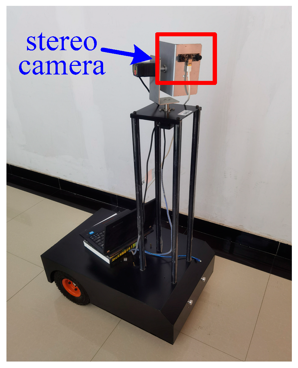
The Zhang calibration method was used to perform an accurate calibration. A high-precision (0.1 mm) standard calibration plate with 15 × 11 grids and an edge length of 50 mm and a simulated planetary rover (Figure 10) equipped with stereo navigation cameras were used. In this study, 13 image pairs were obtained at a fixed focal length. Then, the stereo camera was calibrated using MATLAB calibration toolbox [43]. The calibration process is mainly composed of three steps, i.e., corner detection, calibration of IO and EO elements and distortion parameters, and optimal solution calculation via reprojection.

We analyzed the calibration results by re-projection error. The statistical results can be concluded that the average error of reprojection obtained by using 13 pairs of images is 0.3 pixels. The reprojection error of Camera 1 was slightly larger than that of Camera 2, indicating that the quality of Camera 1 was lower than that of Camera 2. Moreover, the reprojection errors of the 13th image pair were above 0.4 pixels. To obtain accurate calibration results, the 13th image pair was discarded. After that, the reprojection error of the left and right cameras was reduced to 0.2 pixels. The IO elements and distortion parameters obtained during calibration are shown in

Table 1. Laboratory calibration results of the navigation cameras.

Parameters	Left Camera	Right Camera
Focal length f (pixel)	976.5	968.3
$\mathrm{Coordinate} \mathrm{of} \mathrm{principal} \mathrm{point} u_0$ (pixel)	−45.6	7.0
$\mathrm{Coordinate} \mathrm{of} \mathrm{principal} \mathrm{point} v_0$ (pixel)	−11.1	0.2
$\mathrm{Radial} \mathrm{distortion} k_1$	0.2	0.2
$\mathrm{Radial} \mathrm{distortion} k_2$	−0.4	−0.3
$\mathrm{Tan}\mathrm{gential} \mathrm{distortion} p_1$	−1.6 × 10−4	1.7 × 10−3
$\mathrm{Tan}\mathrm{gential} \mathrm{distortion} p_2$	−2.2 × 10−3	−1.4 × 10−3

.

After the calibration, the camera parameters could be used as the initial values of the proposed combined adjustment method. The method mainly includes four steps: (1) extraction of the coordinates of the virtual control points and the matching points, (2) determination of the initial EO elements, (3) self-calibration bundle adjustment with multiple constraints, and (4) accuracy assessment.

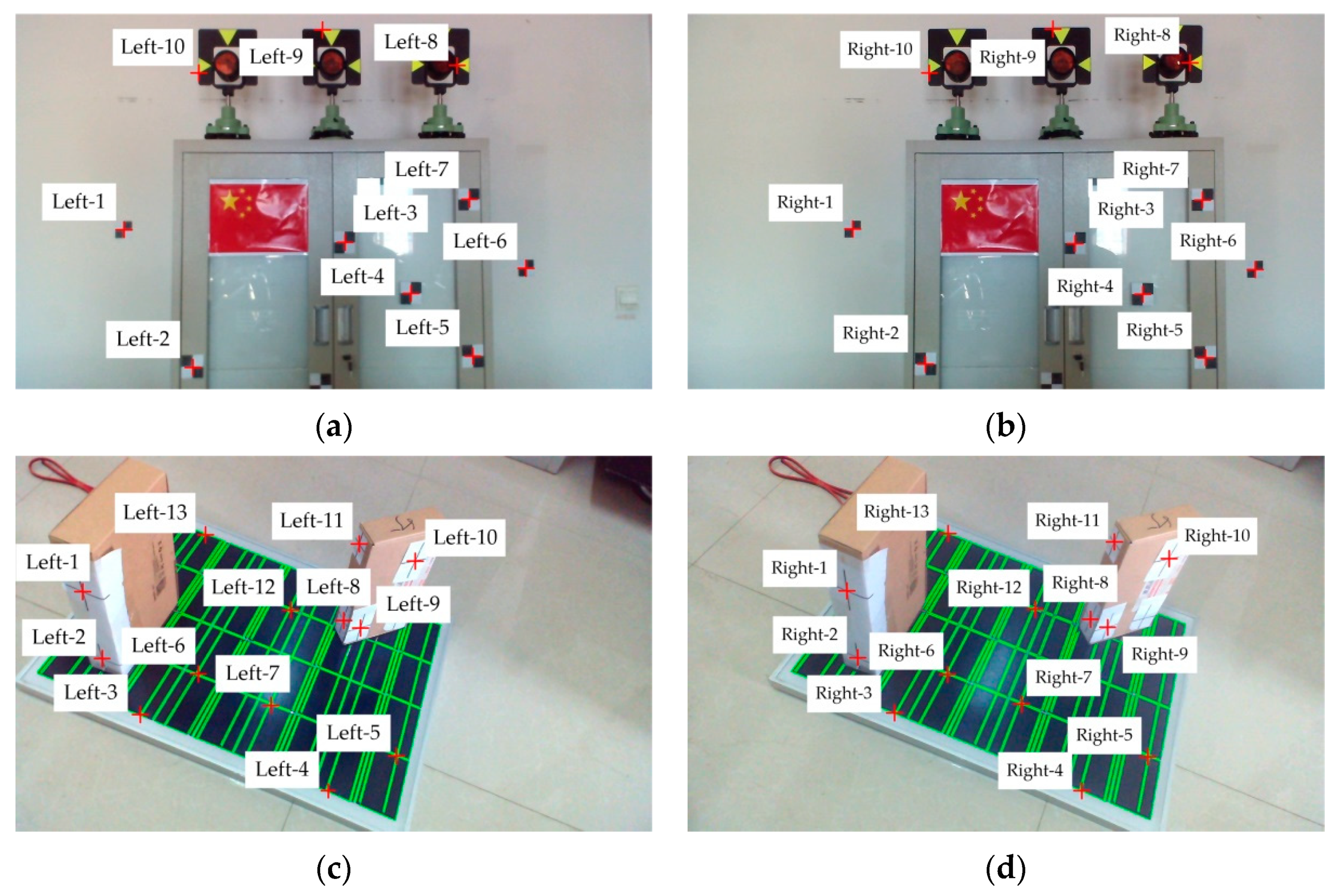
Specifically, the image point coordinate extraction software was used to extract the coordinates of the virtual control points with sub-pixel precision. Then the proposed method in Section 2.3 was used to extract the straight line of the solar panel area. There were 10 pairs of virtual control points in the lander images and 13 pairs in the solar panel images. The virtual control points are shown in Figure 11. Since it is impossible to simulate the actual lighting environment of solar panels, the comparison experiment of line extraction is implemented in Section 3.3.

Before adjustment, the initial value of EO must be obtained. In this study, the DLT algorithm was used to calculate the initial values of the EO elements. The error equations of the left and right images were constructed separately.

Based on the above initial data, the proposed self-calibration bundle adjustment model with multiple constraints was used to carry out parameters calibration, and the LM algorithm was used for adjustment. Since the first image pair did not contain line features, only distance and coplanar constraint conditions were used. The model converged after 10 iterations, and the unit weight RMSE was 2.0 mm. The average reprojection error of the images was 2.7 pixels by the left and right camera. The second image pair contained line features, so collinear constraint was included in the calibration. The adjustment was then carried out based on the two pairs of images, and RMSE was reduced to 1.0 mm. The average reprojection error of the images was 1.1 pixels by the left camera and 0.9 pixels by the right camera. The average reprojection error indicated that the accuracy of the result was higher when the collinear constraint was included (using two pairs of images). Thus, the use of collinear constraints can effectively improve the accuracy of the calibration parameters.

The errors of calibration results when using one pair and two pairs of stereo images are shown in

Table 2. RMSE of calibration results.

Parameters	One Image Pair		Two Image Pairs
	Left Camera	Right Camera	Left Camera	Right Camera
f (pixel)	2.9	2.4	1.6	−1.4
$u_0$ (pixel)	2.8	−1.9	−1.5	−1.1
$v_0$ (pixel)	−2.7	−0.7	−1.3	0.3
$k_1$	−2.7 × 10−3	2.0 × 10−2	1.5 × 10−3	−1.4 × 10−2
$k_2$	3.4 × 10−2	7.1 × 10−2	−1.5 × 10−2	−6.2 × 10−2
$p_1$	5.3 × 10−5	−6.6 × 10−4	2.3 × 10−5	2.8 × 10−4
$p_2$	−8.3 × 10−4	9.1 × 10−4	−3.7 × 10−4	5.1 × 10−4

.

Table 2 shows the RMSE of each parameter after the adjustment of the two pairs of images, and it was substantially lower than that of the first image pair. Among the key parameters, the relative accuracy of the camera focal length f increased by 43.6% on average, the coordinates of the principal points $u_0$ and $v_0$ increased by 44.6% and 49.7%, respectively, and $k_1$, $k_2$, $p_1$, and $p_2$ increased by 38.4%, 34.1%, 56.6%, and 50.1%, respectively. Thus, the addition of a collinear constraint significantly improved the calibration results. In addition, since there were more constraints for calibration using two pairs of images, this approach is beneficial to the calibration of the parameters.

To verify the accuracy of the calibration results, the proposed method was compared with the classic self-calibration bundle adjustment method, CAHVOR, and Vanishing Points. The results of these methods were compared with the coordinates obtained by the total station measurement system.

Table 3. Errors of the 20 checkpoints.

Methods	Error (mm)
	Average	Max	RMS
The proposed method	0.7	1.1	0.9
Self-calibration bundle adjustment	0.8	1.5	1.2
CAHVOR [30]	1.2	1.6	1.5
Vanishing Points [17]	1.4	2.0	1.6

shows the errors at 20 checkpoints obtained by different methods.

Table 3 shows that the proposed method had a higher accuracy than the other three methods, with an average error of less than 1 mm. Compared with the other three methods, the accuracy of our method is improved by 25.0%, 40.0%, and 43.8% respectively. The error of the bundle adjustment method was slightly larger than that of the proposed method and the errors of CAHVOR and vanishing points were much larger.

The above results show that the proposed method can effectively realize camera calibration using multiple pairs of images. The constraints increased the robustness of the calibration results and the accuracy of the parameters. Thus, it can perform the calculation and inspection of the IO elements and lens distortion in the stereo camera under the in-orbit condition.

3.2. Experiments in Simulated Lunar Environment

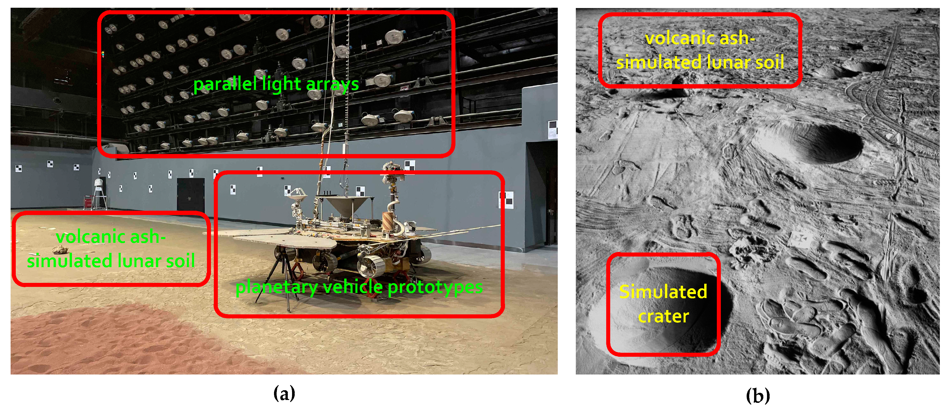
To simulate the various working conditions of the planetary rover in a real deep space environment, the CAST has established a large indoor test field with parallel light arrays, volcanic ash-simulated lunar soil, rocks, craters, and various types of planetary vehicle prototypes. Figure 12 shows the indoor test field and the prototype rover.

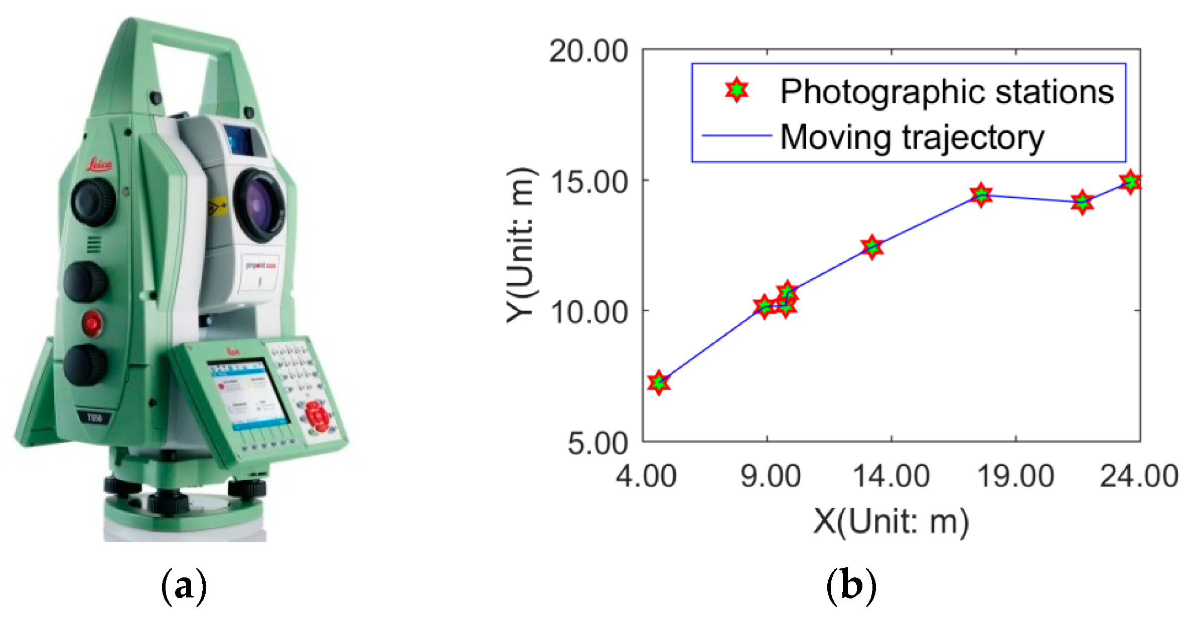
The prototype rover took eight pairs of images at different photographic stations of the indoor test field. Sixty-four checkpoints were arranged in the field of view of the stereo navigation cameras to verify the calibration accuracy. The coordinates of the checkpoints were measured with a high-precision total station measurement system (Leica TS50, Figure 13a), and the angle measurement accuracy was 0.5 s. Figure 13b shows the moving trajectory of the planetary rover and the photographic stations. Figure 14 shows the 64 checkpoints for stereo cameras.

The stereo navigation cameras of the Chang’e-3 prototype were used to collect 27 pairs of stereo images for calibration. Then, the proposed model was used (without the collinear constraint since the prototype was not equipped with solar panels) to verify the IO elements and the radial and tangential distortion parameters. The calibrated parameters of the stereo navigation cameras are shown in

Table 4. Calibration results of the navigation cameras.

Parameters	Calibration Results Using the Calibration Board		Calibration Results of the Proposed Method
	Left Camera	Right Camera	Left Camera	Right Camera
f (pixel)	1181.4	1196.6	1175.3	1192.0
$u_0$ (pixel)	3.1	−1.0	5.9	−6.0
$v_0$ (pixel)	11.5	−18.4	8.4	−14.1
$k_1$	−2.2 × 10−8	−2.2 × 10−8	−3.0 × 10−8	−3.0 × 10−8
$k_2$	3.1 × 10−14	3.1 × 10−14	3.0 × 10−14	3.3 × 10−14
$p_1$	1.5 × 10−7	−5.3 × 10−9	1.9 × 10−7	−5.3 × 10−9
$p_2$	−3.1 × 10−7	−2.6 × 10−7	−4.5 × 10−7	−3.7 × 10−7

.

According to the calibration results, it can be concluded that the differences in the calibration parameters of the proposed method and the calibration plate were between 2.8 pixels and 6.2 pixels. Specifically, the differences in the focal length f of the left and right cameras were 6.2 pixels and 4.6 pixels, respectively, the differences in the coordinates of principal points $u_0$ and $v_0$ were 2.8 pixels, 5.0 pixels, 3.1 pixels, and 4.3 pixels, respectively, and the results of $k_1$, $k_2$, $p_1$, and $p_2$ were close.

Since the calibration method based on the calibration plate and the proposed method are different types of models, it is difficult to directly compare the accuracy from the differences. Therefore, checkpoints were used to verify the accuracy of the results. The space intersection appropriate for multi-images was used to calculate the coordinates of 64 checkpoints in the object coordinate system. Taking the coordinates of the checkpoints measured by the total station measurement system as the true values, the calibration results of the four methods were compared, and the results are shown in

Table 5. Errors of the 64 checkpoints.

Method	Error (mm)
	Average	Max	RMS
The proposed method	2.6	4.5	2.8
Self-calibration bundle adjustment	3.8	6.1	4.4
CAHVOR [30]	5.2	11.0	5.1
Vanishing Points [17]	4.8	8.0	5.0

.

From the statistical results of checkpoint errors, it can be concluded that the proposed method with multiple constraints was significantly more accurate than the self-calibration bundle adjustment model, which was more accurate than the other two methods. Compared with the other three methods, the average accuracy increased by 31.58%, 49.72%, and 45.50%, the maximum error decreased by 26.46%, 59.11%, and 43.41%, and the RMS decreased by 36.44%, 45.09%, and 43.86%. Overall, the proposed method was 42.27%, 42.99%, and 42.35% better than the other methods. The test results indicated that the constraints improved the robustness and accuracy of the adjustment model, and the proposed multiple constraints were effective.

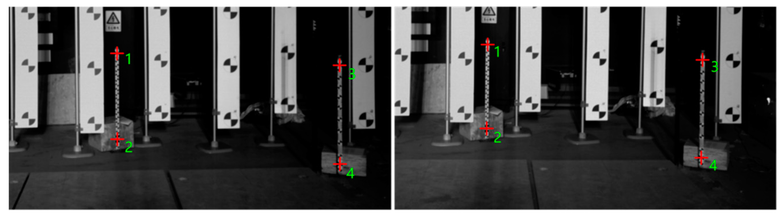
Four pairs of checkpoints in Figure 15 were used for verification. The distance was calculated based on their coordinates obtained by the adjustment. The accuracy of the distance is shown in

Table 6. Distance between checkpoints and the error.

No.	Measurement Value (mm)	Calculated Value (mm)	Difference (mm)
1–2	983.7	985.5	1.8
1–3	1973.6	1972.4	1.2
3–4	1014.6	1013.0	1.7
2–4	1958.4	1957.5	0.9

.

According to the statistical results of the distance error, it can be concluded that the distance deviation between checkpoints was between 0.9 mm and 1.8 mm, with an average deviation of 1.4 mm. Thus, the camera parameters and checkpoint coordinates calculated by the proposed method have high accuracy, demonstrating the reliability of the proposed method.

3.3. In-Orbit Calibration and Analysis

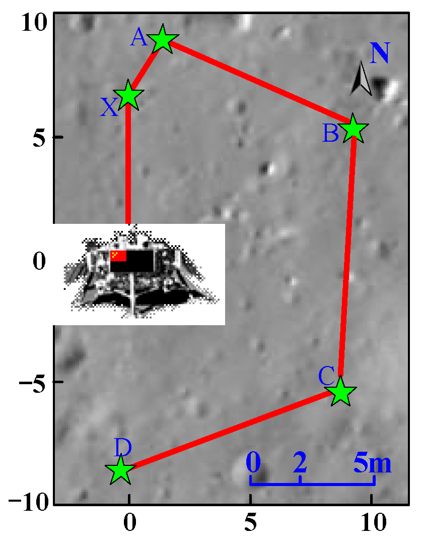
After the planetary rover separated from the lander, it adjusted its moving direction and took sequential images at five photographic stations, i.e., photographic stations X, A, B, C and D (Figure 16). Ten pairs of stereo images from the top of the lander, photographic stations C and D are used to verify the effectiveness of the proposed method under in-orbit conditions.

The in-orbit calibration process of the navigation cameras can be divided into four steps: (1) extraction of the image point coordinates of the virtual control points and the matching connection points, (2) calculation of the initial EO elements, (3) self-calibration bundle adjustment with multiple constraints, and (4) accuracy assessment. Since no checkpoints with known coordinates were on the lunar surface, the accuracy of the camera parameters was evaluated based on the dimensions of the devices on the rover and the positioning results of the planetary rover.

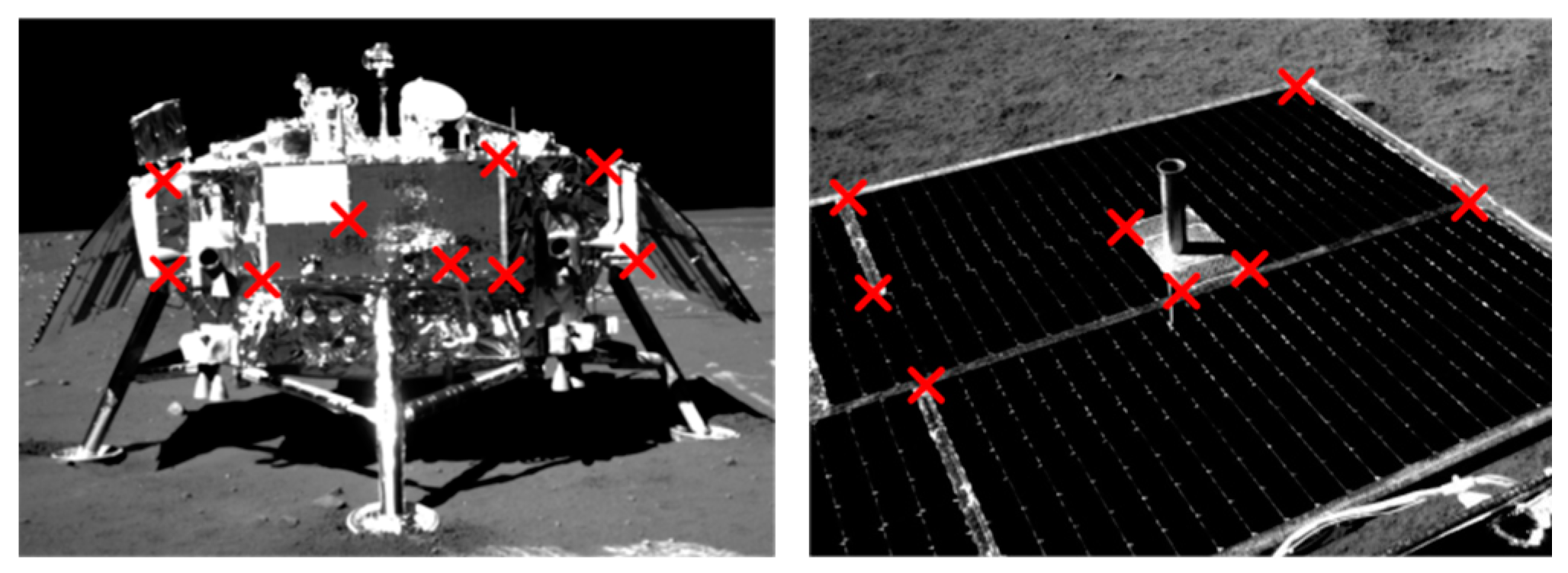
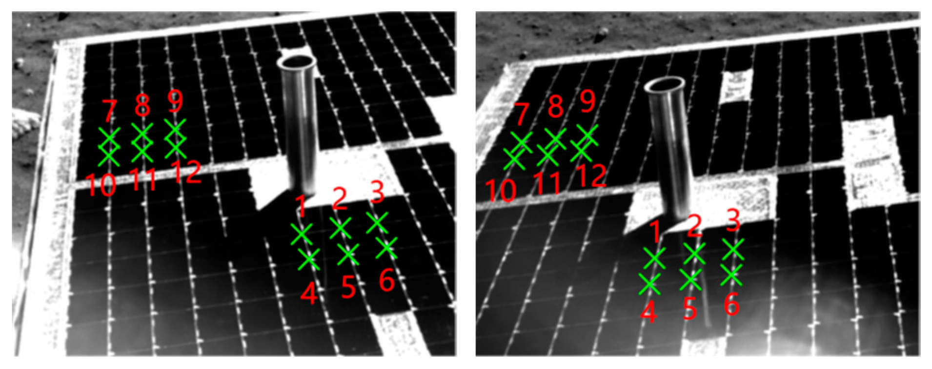
(1) Manual extraction of the coordinates of the virtual control points. The sub-pixel coordinate extraction of the connecting points is carried out with the software specially designed for the Chang’e-3 mission. A total of 9 pairs of connection points were extracted from the images taken at station D and were taken as the control points. Another 8 pairs of feature points were extracted as distance constraints from the images of the solar panel taken at station C. Figure 17 shows the distribution of virtual control points on the solar panel of the lander and planetary rover whose coordinates are measured on the ground.

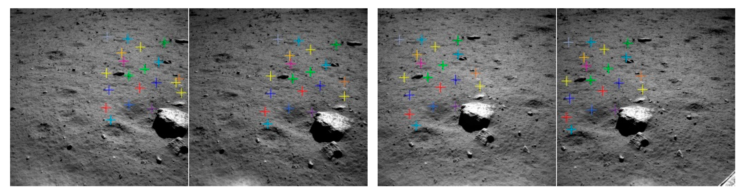
(2) Automatic matching of the connection points. The parameters to be solved included the position and orientation of the camera and the virtual control points were not uniformly distributed in the image; therefore, to improve the accuracy of the model solution, the stereo images were matched to build a set of connection points. Figure 18 shows the matching results of two pairs of stereo images.

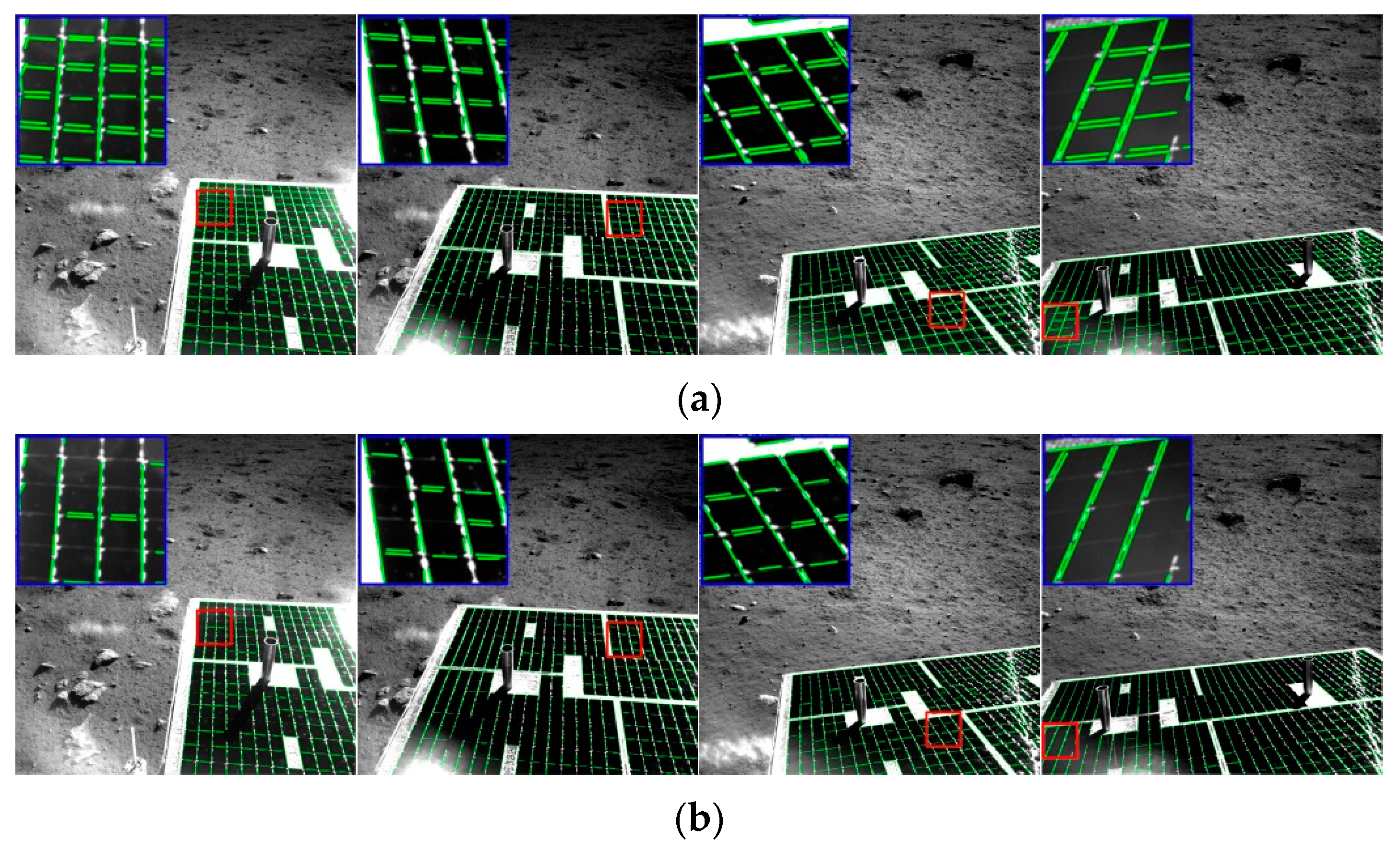
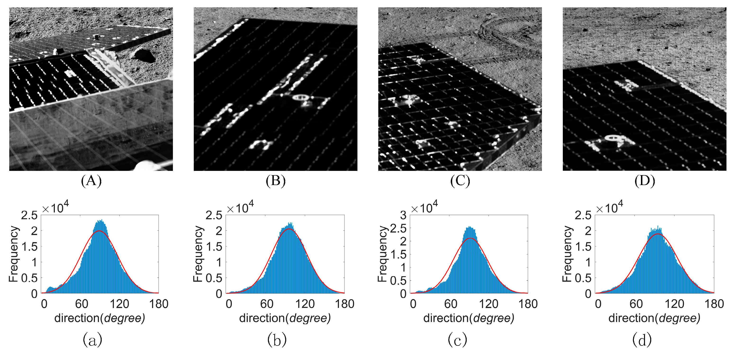
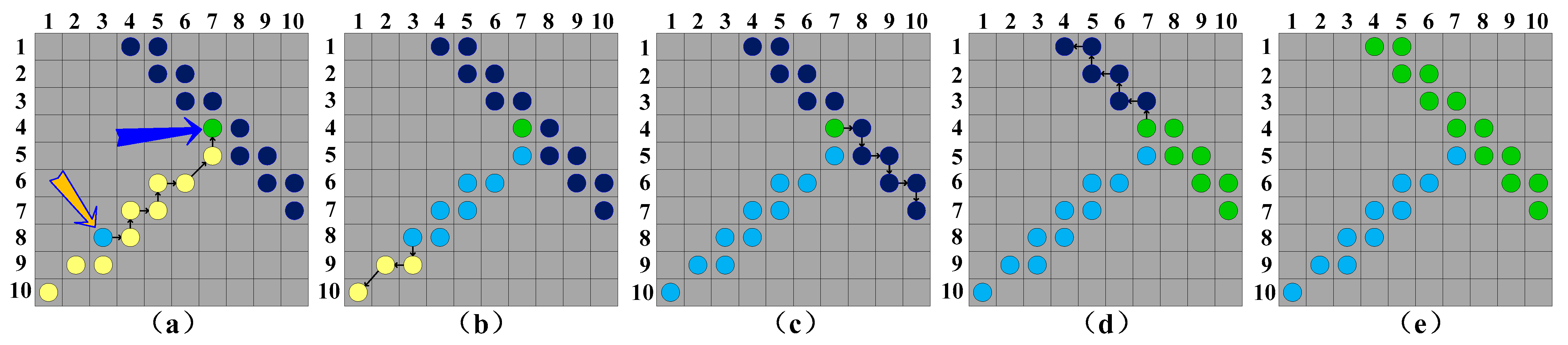
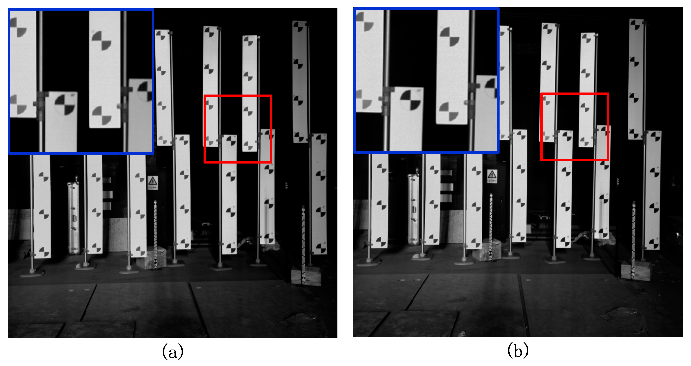
(3) Extraction of line features on the solar panel. The adaptive line extraction method proposed in Section 2.3 was used to extract the line features in the images of the solar panel. Figure 19 shows the result of line extraction using the proposed method and the classic LSD (line segment detector) method.

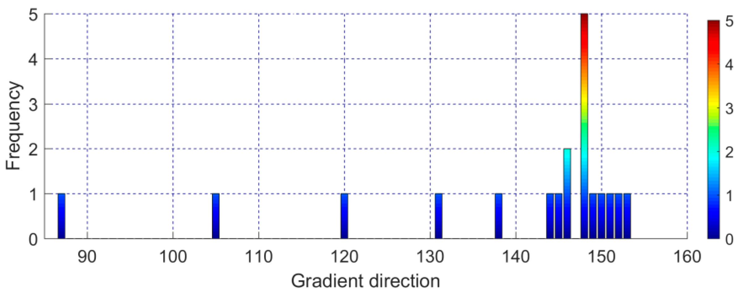
The results show that the proposed method extracted more lines. Especially, the lines with smaller gradients were also extracted. The main reason was that the threshold of the proposed method was adaptively determined according to the gradient direction of the line, which effectively overcame the problem that the global unified threshold cannot be used for extraction because of the large brightness difference in the solar panel area in the stereo image due to the color and illumination.

According to the extracted coordinates of the image point, the coordinates of the connection point, and the initial camera parameters obtained before launching, the initial EO elements were solved by the DLT algorithm. Then, the self-calibration bundle adjustment method with multiple constraints was used for 3 image pairs of the top of the lander and 7 image pairs from each of photographic stations C and D. The IO elements and distortion parameters and the corresponding RMSEs obtained by the combined adjustment are shown in

Table 7. In-orbit calibration results of the navigation cameras.

IO and RMSE	f (Pixel)	${\mathit{u}}_0 \left(\mathbf{Pixel}\right)$	${\mathit{v}}_0 \left(\mathbf{Pixel}\right)$	${\mathit{k}}_1$	${\mathit{k}}_2$	${\mathit{p}}_1$	${\mathit{p}}_2$
IO of the left camera	1194.2	−6.1	−9.8	−4.3 × 10−8	5.6 × 10−14	7.2 × 10−7	−4.6 × 10−7
RMSE of the left camera	0.1	0.2	0.1	2.3 × 10−8	3.1 × 10−9	4.3 × 10−8	3.3 × 10−7
IO of the right camera	1180.1	9.5	7.7	−3.0 × 10−8	5.8 × 10−14	−8.6 × 10−8	−6.5 × 10−7
RMSE of the right camera	0.1	0.2	0.2	3.9 × 10−8	4.5 × 10−9	3.7 × 10−8	2.3 × 10−7

.

Table 7 shows that the proposed method obtained the camera’s IO elements and distortion parameters with high accuracy. The average RMSE of focal length f and coordinates of the principal points $u_0$ and $v_0$ was only 0.1 pixel, 0.2 pixels, and 0.2 pixels, respectively. Thus, the proposed method was feasible under in-orbit conditions and can provide technical references for in-orbit calibration of planetary rovers in deep space exploration missions.

Furthermore, the influence of different constraints on the calibration was analyzed. Combining the above observations and different constraints, 7 different models were established. Since the same points are used for collinear and coplanar constraints, both are used as constraints at the same time. Finally, the median errors of various models are obtained after adjustment, and the details are shown in

Table 8. Comparison of different model elements.

Method	Unknown Variables	Number of Equations	Redundant Observations	$\mathbf{Standard} \mathbf{Deviation} {\mathit{\sigma }}_0 \left(\mathbf{Pixel}\right)$
BA	1847	2272	425	1.671
BA + DC	1847	2336	489	1.541
BA + CCC	1847	2944	1097	1.024
BA + RC	1847	3088	1241	0.978
BA + DC + CCC	1847	3008	1161	0.996
BA + CCC + RC	1847	3760	1913	0.787
BA + DC + CCC + RC	1847	3824	1977	0.763

Note: BA means bundle adjustment, DC means distance constraint, CCC means collinear and coplanar constraint, RC means relative pose constraint.

.

From the above experimental results, it can be concluded that BA can be solved without constraints, but the standard deviation is larger than other models with additional constraints, indicating that the proposed constraints are beneficial to the adjustment.

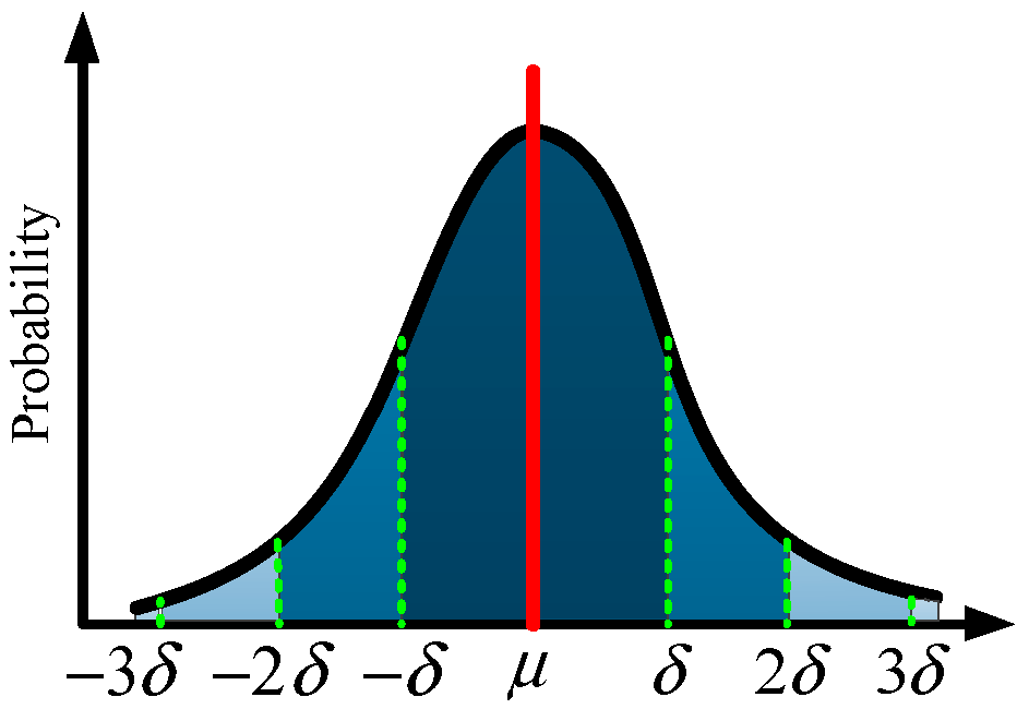
Compared with the BA, the standard deviation of the various models with different constraints is reduced by 8%, 61%, 63%, 62%, 75%, and 76%, respectively, indicating that the accuracy of the proposed method is significantly improved. Since there are more redundant observations than other models, CCC and RC have a greater effect on the improvement of calibration accuracy. we found the sums of squared residuals of BA with different additional constraints are pretty close. The larger the redundancy number, the smaller the estimation precision ${\sigma }_0$ of calibration parameters. So the redundancy number of BA with different additional constraints is larger than that of BA. Thus, the calibration parameters estimation precision of BA with different additional constraints is better, and the adoption of various models proposed in this paper as geometric constraints is more rational.

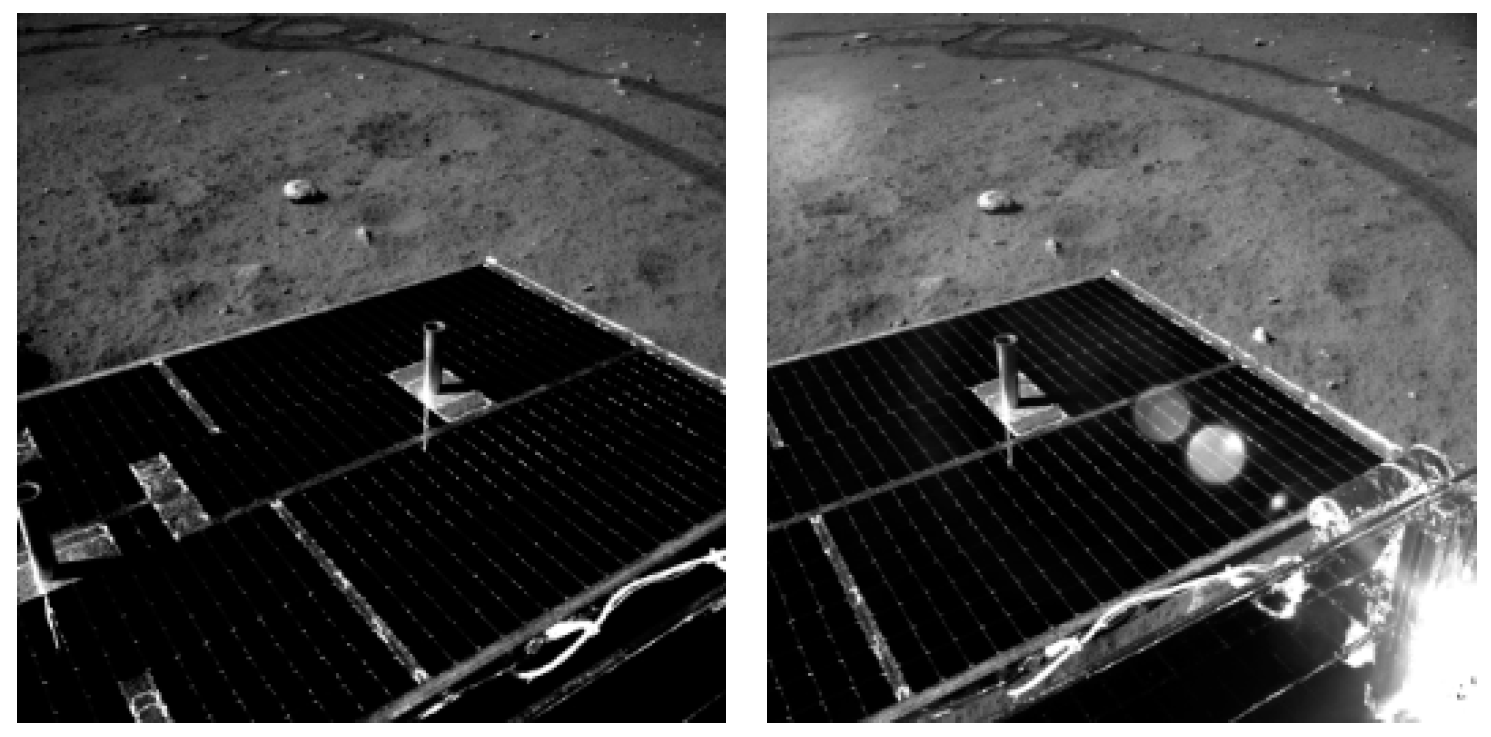
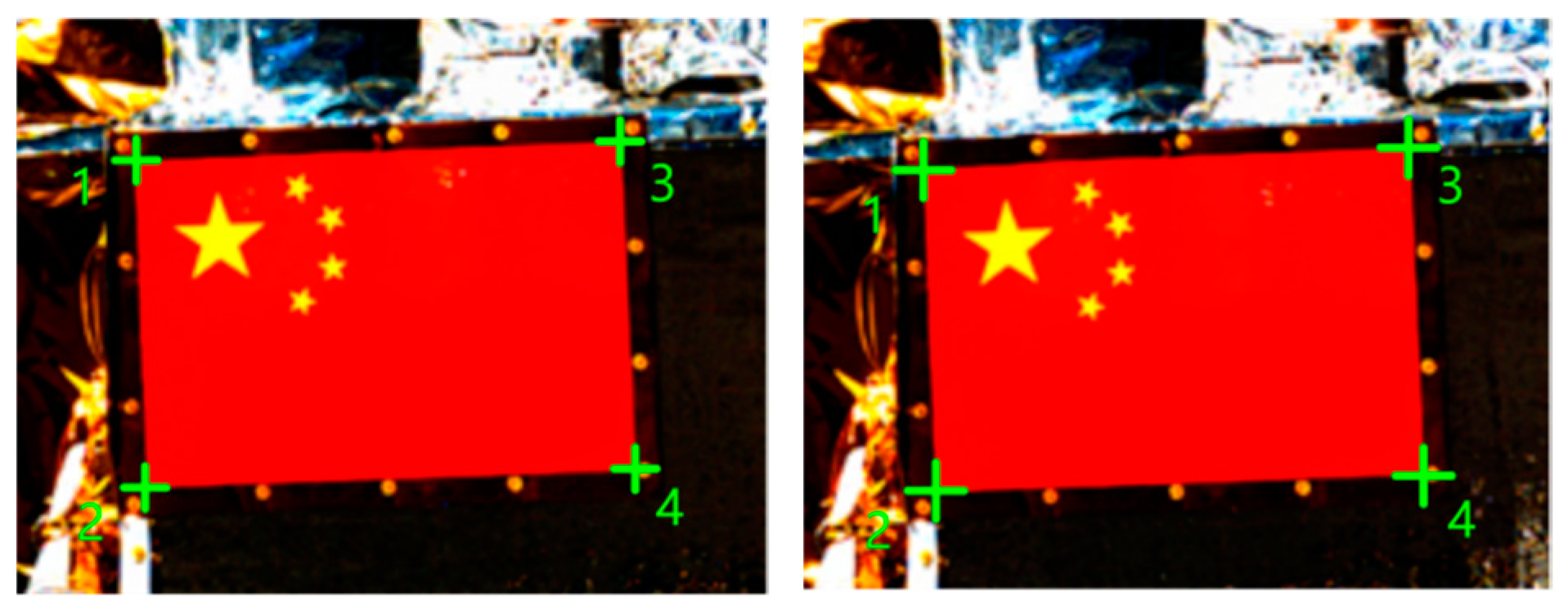
In addition, the accuracy of the parameters was indirectly verified using the size of the national flag. Figure 20 shows the manually extracted corner points of the national flag, and

Table 9. Verification of the dimensions of the flag on the lander.

Point	Designed Value (mm)	Calculated Value (mm)	Deviation (mm)
1–2	210.0	211.5	−1.5
2–4	297.0	296.8	0.2
3–4	210.0	209.4	0.6
3–1	297.0	298.4	−1.4
1–4	363.7	364.2	−0.4
2–3	363.7	365.7	−2.0

shows the design size and calculated size of the national flag and the differences.

According to Table 9, the calculation errors were not more than 2 mm, indicating that using the IO elements and distortion parameters calculated by the proposed method to solve the space coordinates of other points can achieve good accuracy.

Based on the line extraction results of the solar panel from images taken by stereo cameras at different photographic stations and angles, the coordinates of the intersection points between lines, and the calculated parameters, the lengths of multiple OSRs were calculated and compared with the true value. Figure 21 shows the endpoints of the OSRs after line extraction. The length and width of the OSR obtained by the 3D coordinates calculated by the binocular vision measurement method were compared with the design values, as shown in

Table 10. Calculated OSR dimensions of solar panel and errors.

No.	Calculated (mm)	Designed (mm)	Deviation (mm)	No.	Calculated (mm)	Designed (mm)	Deviation (mm)
1–2	31.6	31.5	−0.1	7–8	31.9	31.5	−0.4
2–3	30.9	31.5	0.6	8–9	31.0	31.5	0.5
4–5	31.6	31.5	−0.1	10–11	31.0	31.5	0.5
5–6	31.0	31.5	0.5	11–12	30.9	31.5	0.6
1–4	39.7	40.3	0.6	7–10	39.4	40.3	0.9
2–5	38.9	40.3	1.4	8–11	38.8	40.3	1.5
3–6	41.1	40.3	−0.8	9–12	41.0	40.3	−0.7

.

Table 10 shows that the calculated OSR dimensions from images of different angles and distances were accurate. The average length of calculated by the parameters obtained by the proposed method was 31.2 mm, and the average width was 39.8 mm, with an average deviation from the designed value of 0.4 mm and 1.0 mm, respectively. Thus, the camera parameters obtained by the proposed method have good accuracy. In particular, the lens distortion parameters have good reliability and accuracy.

In summary, the classic bundle adjustment model has good accuracy. However, in the absence of constraints, the point position may still deviate in the light direction during the adjustment process. With the addition of distance constraints and coplanar constraints, the spatial geometric structure of the observations is more stable and reliable, thereby reducing the point deviation during the solution, and ultimately improving the accuracy of camera parameter calibration. In addition, the relative pose constraints of the left and right navigation cameras can also realize the spatial geometric constraints of the EO, making the model during the adjustment more stable and the solution more accurate.

4. Conclusions

Accurate IO elements of the stereo camera are crucial for the in-orbit navigation and positioning of planetary rovers. High-precision in-orbit parameter calibration can provide a reference for path planning of the planetary rover and play a key role in ensuring the safety of the planetary rover and improving the efficiency of scientific missions. In deep space exploration missions, the variables that can be used for in-orbit camera calibration are very limited. Therefore, an in-orbit stereo camera self-calibration method of planetary rovers with multiple constraints was proposed. Based on the bundle method of the binocular stereo camera, four types of constraints were included to construct the self-calibration bundle adjustment model with multiple constraints, i.e., the constraint of the distance between feature points on the lander and the planetary rover, the collinear constraint of the connection points on the solar panel, the coplanar constraint of feature points on the solar panel and national flag, and the relative position and orientation constraint of the left and right cameras. Given the problem of unsatisfactory distribution of line gradient features in the solar panel images, an adaptive line extraction method based on brightness weighting was proposed to ensure the accuracy of line extraction in different directions. Through various types of experiments, the following conclusions were obtained:

(1) In the simulations in a general laboratory, two pairs of stereo images were used in the adjustment. The results showed that using the extracted linear features as additional constraints can effectively improve the accuracy of the obtained camera parameters, and the reprojection error was reduced to 1.0 pixels. Overall, the accuracy of various parameters was improved by 34.1–56.6%.

(2) In the experiments at the simulated experimental field built by CAST, 64 checkpoints were used to test the calibration accuracy. The results showed that the average error of the proposed method was only 2.1 mm, which was 31.58%, 49.72%, and 45.50% better than the classic self-calibration bundle adjustment method, CAHVOR, and Vanishing Points, respectively. Four pairs of checkpoints were selected for distance verification, and the average distance error was only 1.4 mm.

(3) In the in-orbit calibration test of the Chang’e-3 planetary rover, the average RMSE of the focal length and the principal point coordinates was only 0.2 pixels for the left camera and right camera. The maximum error in flag dimensions was 2.0 mm and the minimum error was 0.2 mm. The maximum error in the length of the OSR of the solar panel was 1.5 mm, and the minimum error was 0.1 mm.

Based on the above results, the proposed method can obtain high-precision IO elements and lens distortion parameters of the stereo cameras under in-orbit conditions, which provide a reference for in-orbit camera calibration of planetary rovers in the deep space exploration missions of all countries.

References

1. Shi, P.; Wang, Q.; Bai, Q.; Fan, Q. Review of 2020 global deep space activities. Sci. Technol. Rev. 2021, 39, 69–87. [Google Scholar]
2. Liu, J.; Hu, C.; Pang, F.; Kang, Y.; Li, H.; Ma, J.; Lu, X. Strategy of deep space exploration. Sci. Sin. Technol. 2020, 50, 1126–1139. (In Chinese) [Google Scholar] [CrossRef]
3. Chen, L.; Zhao, C. China successfully launched its first mars mission, Tianwen 1. Aerosp. China 2020, 21, 51. [Google Scholar]
4. Di, K.; Liu, B.; Xin, X.; Yue, Z.; Ye, L. Advances and applications of lunar photogrammetric mapping using orbital images. Acta Geod. Cartogr. Sin. 2019, 48, 1562–1574. [Google Scholar]
5. Ma, Y. Research on Navigation and Positioning Technology of Chang’e-3 Lunar Patrol Probe. Ph.D. Thesis, Wuhan University, Wuhan, China, 2014. [Google Scholar]
6. Abdel-Aziz, Y.I.; Karara, H.M.; Hauck, M. Direct linear transformation from comparator coordinates into object space coordinates in close-range photogrammetry. Photogramm. Eng. Remote Sens. 2015, 81, 103–107. [Google Scholar] [CrossRef]
7. Tsai, R. A versatile camera calibration technique for high-accuracy 3D machine vision metrology using off-the-shelf TV cameras and lenses. IEEE J. Robot. Autom. 2003, 3, 323–344. [Google Scholar] [CrossRef] [Green Version]
8. Weng, J. Camera calibration with distortion models and accuracy evalution. IEEE Trans. Pattern Anal. Mach. Intell. 1992, 14, 965–980. [Google Scholar] [CrossRef] [Green Version]
9. Faugeras, O.D.; Luong, Q.T.; Maybank, S.J. Camera self-calibration: Theory and experiments. In Proceedings of the European Conference on Computer Vision, Santa Margherita Ligure, Italy, 19–22 May 1992; pp. 321–334. [Google Scholar]
10. Maybank, S.; Faugeras, O. A theory of self-calibration of a moving camera. Int. J. Comput. Vis. 1992, 8, 123–151. [Google Scholar] [CrossRef]
11. Martinez-Perez, M.E.; Espinosa-Romero, A. Three-dimensional reconstruction blood vessels extracted from retinal fundus images. Opt. Express 2012, 20, 11451–11465. [Google Scholar] [CrossRef]
12. Jiang, Z.; Jia, L.; Guo, S. Research on camera self-calibration of high-precision in binocular vision. Procedia Eng. 2012, 29, 4101–4106. [Google Scholar] [CrossRef] [Green Version]
13. Merras, M.; Akkad, N.E.; Saaidi, A.; Nazih, A.G.; Satori, K. A new method of camera self-calibration with varying intrinsic parameters using an improved genetic algorithm. In Proceedings of the 2013 8th International Conference on Intelligent Systems: Theories and Applications (SITA), Rabat, Morocco, 8–9 May 2013. [Google Scholar]
14. Zhang, Z. A flexible new technique for camera calibration. IEEE Trans. Pattern Anal. Mach. Intell. 2000, 22, 1330–1334. [Google Scholar] [CrossRef] [Green Version]
15. Tan, X.; Yu, Z.; Li, J. An improved method of stereo camera calibration. Acta Geod. Cartogr. Sin. 2006, 35, 138–142. [Google Scholar]
16. Shi, Z.C.; Shang, Y.; Zhang, X.F.; Wang, G. DLT-lines based camera calibration with lens radial and tangential distortion. Exp. Mech. 2021, 61, 1237–1247. [Google Scholar] [CrossRef]
17. Caprile, B.; Torre, V. Using vanishing points for camera calibration. Int. J. Comput. Vis. 1990, 4, 127–139. [Google Scholar] [CrossRef]
18. Wei, G.Q.; He, Z.; Ma, S.D. Camera calibration by vanishing point and cross ratio. In Proceedings of the International Conference on Acoustics, Speech, and Signal Processing, Glasgow, UK, 23–26 May 1989; pp. 1630–1633. [Google Scholar]
19. Fan, H. Research and Application of Wide Angle Camera Calibration based on Concentric Circles. Master’s Thesis, Xidian University, Xi’an, China, 2015. [Google Scholar]
20. Zhao, L.; Wu, C. Camera calibration method based on circular points. J. Xidian Univ. 2007, 3, 363–367. [Google Scholar]
21. Peng, Y.; Guo, J.; Yu, C.; Ke, B. High precision camera calibration method based on plane transformation. J. Beijing Univ. Aeronaut. Astronaut. 2021, 9, 1–10. [Google Scholar]
22. Brown, D.C. A Solution to the General Problem of Multiple Station Analytical Stereotriangulation; Rca-mtp Data Reduction Technical Report no. 43; Patrick Airforce Base: Brevard County, FL, USA, 1958. [Google Scholar]
23. Huang, W.; Jiang, S.; Jiang, W. Camera self-calibration with GNSS constrained bundle adjustment for weakly structured long corridor UAV images. Remote Sens. 2021, 13, 4222. [Google Scholar] [CrossRef]
24. Zheng, S.; Huang, R.; Guo, B.; Hu, K. Stereo-camera calibration with restrictive constraints. Acta Geod. Cartogr. Sin. 2012, 41, 877–885. [Google Scholar]
25. Xie, L.; Hu, H.; Wang, J.; Zhu, Q.; Chen, M. An asymmetric re-weighting method for the precision combined bundle adjustment of aerial oblique images. J. Photogramm. Remote Sens. 2016, 117, 92–107. [Google Scholar] [CrossRef]
26. Liu, S.C.; Jia, Y.; Ma, Y.Q.; Gu, Z.; Wei, S.Y.; Li, Q.Z.; Xu, X.C.; Wen, B.; Zhang, S.; Li, M.L.; et al. High precision localization of the Chang’E-3 lunar rover. Chin. Sci. Bull. 2015, 60, 372–378. [Google Scholar]
27. Yakimovsky, Y.; Cunningham, R. A system for extracting three-dimensional measurements from a stereo pair of TV cameras. Comput. Graph. Image Process. 1978, 7, 195–210. [Google Scholar] [CrossRef]
28. Bell, J.F., III; Godber, A.; Mcnair, S.; Caplinger, M.A.; Maki, J.N.; Lemmon, M.T.; Van Beek, J.; Malin, M.C.; Wellington, D.; Kinch, K.M.; et al. The Mars science laboratory curiosity rover mast camera (mastcam) instruments: Pre-flight and in-flight calibration, validation, and data archiving: Msl/mastcam calibration. Earth Space Sci. 2017, 4, 396–452. [Google Scholar] [CrossRef] [Green Version]
29. Mahboub, V. On weighted total least-squares for geodetic transformations. J. Geod. 2011, 86, 359–367. [Google Scholar] [CrossRef]
30. Gennery, D.B. Generalized camera calibration including fish-eye lenses. Int. J. Comput. Vis. 2006, 68, 239–266. [Google Scholar] [CrossRef]
31. Workman, S.; Mihail, R.P.; Jacobs, N. A pot of gold: Rainbows as a calibration cue. In Proceedings of the European Conference on Computer Vision, Zurich, Switzerland, 6–12 September 2014; pp. 820–835. [Google Scholar]
32. Wang, H.; Zhang, X.; Li, H. A stereo rectification algorithm for planetary rover visual navigation system. J. Astronaut. 2017, 38, 159–165. [Google Scholar]
33. Xu, X.; Xu, A.; Liu, S.; Ma, Y.; Zheng, Z. A positioning method of rover based on descent image and navigation image. J. Navig. Position. 2017, 5, 32–37. [Google Scholar]
34. Liu, Z.; Wan, W.; Peng, M.; Zhao, Q.; Xu, B.; Liu, B.; Liu, Y.; Di, K.; Li, L.; Yu, T.; et al. Remote sensing mapping and localization techniques for teleoperation of Chang’e-3 rover. Natl. Remote Sens. Bull. 2014, 18, 971–980. [Google Scholar]
35. Doyle, F.J. The historical development of analytical photogrammetry. Photogramm. Eng. Remote Sens. 1964, 30, 259–265. [Google Scholar]
36. Xing, C.; Deng, X.; Li, Y. Seed point optimal selection method of PTD algorithm based on confidence interval estimation theory. Eng. Surv. Mapp. 2020, 29, 27–32. [Google Scholar]
37. Yang, J.; Zhou, J. Restore of Mathematical detail: The process of gauss deriving the probability density function of normal distribution. J. Stat. Inf. 2019, 34, 17–21. [Google Scholar]
38. Yang, N.; Cui, J.; Zhou, Z.; Zhang, S.; Hou, J.; Hu, W. Research on modeling of probability density distribution of transverse wind power time series based on gaussian mixture distribution. Water Resour. Power 2016, 34, 213–216. [Google Scholar]
39. Von Gioi, R.G.; Jakubowicz, J.; Morel, J.M.; Randall, G. LSD: A line segment detector. Image Process. Line 2012, 2, 35–55. [Google Scholar] [CrossRef] [Green Version]
40. Feng, P. Research on Camera Calibration by Self Checking Beam Adjustment Based on Sparse Matrix. Master’s Thesis, Xi’an University of Science and Technology, Xi’an, China, 2014. [Google Scholar]
41. Wang, B.; Liu, C. Computer Vision Technology in Lunar Rover Teleoperation; National Defense Industry Press: Beijing, China, 2016; pp. 26–30, 38. [Google Scholar]
42. Tsai, R.Y. An efficient and accurate camera calibration technique for 3D machine vision. In Proceedings of the IEEE Conference on Computer Vision and Pattern Recognition, Miami Beach, FL, USA, 22–26 June 1986; pp. 364–374. [Google Scholar]
43. Team E. MathWorks releases release2016b with MATLAB and Simulink product families. Appl. Electron. Tech. 2016, 42, 10. [Google Scholar]
Figure 1. Stereo Vision System of Planetary Rovers.
Remotesensing 14 00402 g001
Figure 2. Positioning of binocular stereo cameras.
Remotesensing 14 00402 g002
Figure 3. Images captured by the navigation cameras.
Remotesensing 14 00402 g003
Figure 4. (a) Neighborhood pixels and gradient directions. the numbers 1–8 indicate the 8 neighborhood pixels of the central pixel (i, j) in turn, and 0°, 45°, 90°, and 135° respectively indicate the four gradient directions. (be) are the convolution templates corresponding to the four directions.
Remotesensing 14 00402 g004
Figure 5. (AD) are 4 original images taken by the Chang’e-3 navigation camera. (ad) are the histograms of gradient directions corresponding to 4 images, the red curve in each figure is a Gaussian curve fitted by the statistical results of the histogram. In the histogram, the horizontal axis represents the gradient direction value and the vertical axis represents the number of occurrences.
Remotesensing 14 00402 g005
Figure 6. Gaussian distribution and subintervals of gradient directions.
Remotesensing 14 00402 g006
Figure 7. The histogram of the gradient directions. The horizontal axis means the direction of the gradient (Unit: degree ), and the vertical axis represents the number of occurrences.
Remotesensing 14 00402 g007
Figure 8. (a) is to obtain the seed point of each chain. The blue and green points are the respective seed points of the two chains in the peak gradient direction, and the yellow points indicate other points of the first chain. Dark blue points indicate other points of the second chain (b) means starting from the seed point of a chain, detecting the eligible points along a certain direction, and growing the line until it stops when it encounters the next chain. (c) Means to start from the seed point again and grow the line in the opposite direction until the detection of all points in the chain that meet the conditions is completed, and the preliminary detection of the line is completed. (d,e) is the line detection and growth process of the second chain, the process is the same as that of the first chain.
Remotesensing 14 00402 g008
Figure 9. Connection of lines.
Remotesensing 14 00402 g009
Figure 10. Stereo camera and simulated planetary rover.
Remotesensing 14 00402 g010
Figure 11. In the simulation experiment, (a,b) are the left and right images of the first photographic station and the corresponding virtual control point distribution. (c,d) are the left and right images, virtual control points and the extracted linear features of the second photographic station.
Remotesensing 14 00402 g011
Figure 12. (a) Is the overall environment of the test site, including parallel light arrays, simulated lunar soil and planetary vehicle prototypes. (b) Is the image taken by the navigation camera after turning on the parallel light array in the test field.
Remotesensing 14 00402 g012
Figure 13. (a) Shows the Leica TS50 high-precision total station measurement system. The source of the photo of the Leica TS50 was taken from the official Leica product manual (b) shows the moving trajectory and photographic positions of the planetary rover during the test.
Remotesensing 14 00402 g013
Figure 14. Checkpoints and stereo images (the subgraph is a detailed display of the red square box area on the right. The intersection of two opposite black areas is the corresponding checkpoint. (a,b) are the images captured by the left and right navigation cameras).
Remotesensing 14 00402 g014
Figure 15. Checkpoints used for distance verification.
Remotesensing 14 00402 g015
Figure 16. The photographic stations and moving trajectory of the planetary rover around the Chang’e-3 lander. The source of the background image was taken by the descent camera.
Remotesensing 14 00402 g016
Figure 17. Distribution of control points on the lander and the solar panel of rover.
Remotesensing 14 00402 g017
Figure 18. Matching results of connection points in images taken at adjacent stereo images (The same color represents the corresponding matching points).
Remotesensing 14 00402 g018
Figure 19. Line extraction results of solar panels by different methods. (a) Is the line detection result of the proposed method. (b) Is the Line extraction result of the LSD method.the subgraph is a detailed display of the red square box area. The green lines are the lines detected by the corresponding method.
Remotesensing 14 00402 g019
Figure 20. Extracted corner points of the national flag.
Remotesensing 14 00402 g020
Figure 21. OSR line intersections.
Remotesensing 14 00402 g021