Article

Polarimetric Persistent Scatterer Interferometry for Ground Deformation Monitoring with VV-VH Sentinel-1 Data

1
Key Laboratory of Land Environment and Disaster Monitoring, MNR, China University of Mining and Technology, Xuzhou 221116, China
2
School of Environment Science and Spatial Informatics, China University of Mining and Technology, Xuzhou 221116, China
3
Guizhou Provincial First Institute of Surveying and Mapping, Guiyang 550025, China
4
Yellow River Engineering Consulting Co., Ltd., Zhengzhou 450000, China
*
Author to whom correspondence should be addressed.
Remote Sens. 2022, 14(2), 309; https://doi.org/10.3390/rs14020309
Submission received: 1 December 2021 / Revised: 24 December 2021 / Accepted: 2 January 2022 / Published: 10 January 2022
(This article belongs to the Special Issue New Technologies for Earth Remote Sensing)

Abstract

:
With the launch of the Sentinel-1 satellites, it becomes easy to obtain long time-series dual-pol (i.e., VV and VH channels) SAR images over most areas of the world. By combining the information from both VV and VH channels, the polarimetric persistent scatterer interferometry (PolPSI) techniques is supposed to achieve better ground deformation monitoring results than conventional PSI techniques (using only VV channel) with Sentinel-1 data. According to the quality metric used for polarimetric optimizations, the most commonly used PolPSI techniques can be categorized into three main categories. They are PolPSI-ADI (amplitude dispersion index as the phase quality metric), PolPSI-COH (coherence as the phase quality metric), and PolPSI-AOS (taking adaptive optimization strategies). Different categories of PolPSI techniques are suitable for different study areas and with different performances. However, the study that simultaneously applies all the three types of PolPSI techniques on Sentinel-1 PolSAR images is rare. Moreover, there has been little discussion about different characteristics of the three types of PolPSI techniques and how to use them with Sentinel-1 data. To this end, in this study, three data sets in China have been used to evaluate the three types of PolPSI techniques’ performances. Based on results obtained, the different characteristics of PolPSI techniques have been discussed. The results show that all three PolPSI techniques can improve the phase quality of interferograms. Thus, more qualified pixels can be used for ground deformation estimation by PolPSI methods with respect to the PSI technique. Specifically, this pixel density improvement is 50%, 12%, and 348% for the PolPSI-ADI, PolPSI-COH, and POlPSI-AOS, respectively. PolPSI-ADI is the most efficient method, and it is the first choice for the area with abundant deterministic scatterers (e.g., urban areas). Benefitting from its adaptive optimization strategy, PolPSI-AOS has the best performances at the price of highest computation cost, which is suitable for rural area applications. On the other hand, limited by the medium resolution of Sentinel-1 PolSAR images, PolPSI-COH’s improvement with respect to conventional PSI is relatively insignificant.

Graphical Abstract

1. Introduction

As a radar remote sensing technique, Persistent Scatterer Interferometry (PSI) [1,2,3,4,5,6,7,8] with Synthetic Aperture Radar (SAR) images can work under all-weather and all-day conditions. Traditional PSI techniques only use persistent scatterers (PSs) pixels, which are with high phase qualities, to retrieve ground deformation. Thus, they can detect and monitor displacements over ground or infrastructures at millimeter level accuracy [9,10] efficiently. Therefore, PSI has been used as a routine tool for terrain deformation monitoring related with subsidence [11,12], mining [13,14,15], earthquakes [16], Volcanoes [17], landslides [18], underground coal fires [19], etc. However, over the areas where distributed scatterers (DSs) are the majority, conventional PSI techniques may encounter the problem of lack of sufficient PS pixels for deformation monitoring. In these places, e.g. the vegetation areas, pixels are strongly affected by decorrelations and therefore have low phase quality, rendering them unsuitable for PSI applications.
As most of the geological environmental hazards occurred at rural areas, the more advanced PSI technique that can take use of distributed scatterers for ground deformation monitoring are invented. This advanced PSI technique is usually named as DS-InSAR, and the first proposed DS-InSAR algorithm is SqueeSAR [20]. After that, many variants of SqueeSAR have been proposed, such as the CAESAR [21] and PD-InSAR [22] methods. DS pixels’ phase optimization is the core of all DS-InSAR approaches, which is usually done by three steps. Firstly, the homogeneous pixels (HPs) of each SAR pixel are identified by using the Kolmogorov–Smirnov (KS) [20], Anderson–Darling (AD) [23] test, or other advanced methods [24]. Then, the number of each pixels’ HPs is employed to classify it into PS and DS pixels. Finally, PS pixels are kept without any processing, whereas DS pixels are optimized with their HPs [20]. Benefited from the adaptive filtering of DS-InSAR techniques, phase qualities of DS pixels have been improved and a part of them are qualified for PSI applications. Thus, more density of pixels can be included for deformation monitoring and more displacement details can be obtained using DS-InSAR algorithms.
On the other hand, inspired by the Polarimetric SAR interferometry (PolInSAR) technique, some researchers proposed to reduce the decorrelation effect by using polarimetric information contained in SAR images [25,26]. As it is known, a certain kind of ground target responds differently to different polarimetric channel SAR images [27]. Thus, by searching for each target’s (pixel’s) optimum scattering mechanism (SM) for InSAR applications, pixels’ interferometric phase noise caused by decorrelations can be reduced. Hence, the first PSI algorithm that employs SAR polarimetric information (named as polarimetric PSI (PolPSI)) has been proposed by Pipia at Universitat Politècnica de Catalunya (UPC), which is based on the Ground-based SAR data [25]. Due to the shortage of long time-series polarimetric SAR (PolSAR) images, the development and applications of PolPSI have been limited. As more and more sattelites with the capability of acquiring PolSAR images (e.g., Radarsat-2, ALOS-2, TerraSAR-X, and Sentinel-1) have been launched, it is possible to extend the PolPSI techniques from the Ground-based SAR images to satellite SAR images. Under this circumstance, more PolPSI algorithms have been proposed [28,29,30,31,32,33,34,35,36,37,38,39].
A phase quality metric has to be chosen for pixels polarimetric optimization in PolPSI. Generally, like the conventional PSI methods, the amplitude dispersion index (ADI, better for PS pixels’ optimization) [26,33,36] and coherence (better for DS pixel optimization) [25,28,29,36] are the two commonly used phase quality metrics. Similarly with DS-InSAR, more advanced PolPSI techniques are proposed to adaptive optimize PS and DS pixels by using the combination of ADI and coherence [31,34,37,38]. Therefore, according to the phase quality metrics used, the most commonly used PolPSI techniques can be classified into three main categories, i.e., PolPSI-ADI (PolPSI with the amplitude dispersion index as the phase quality metric) [26,33,36], PolPSI-COH (PolPSI with the coherence as the phase quality metric) [25,28,29,36], and PolPSI-AOS (PolPSI with the adaptive optimization strategies) [31,34,37,38]. Different PolPSI algorithms are with different phase optimization performances, and suitable for different scenarios [36,37]. Although it is possible to apply PolPSI techniques on satellite SAR images for ground deformation monitoring over broader areas, the free available time-series PolSAR images are far away from enough for PolPSI applications. This is due to the shortcomings of PolSAR systems, especially for the full polarization ones, relative to single polarization SAR systems.
This problem has been partially solved by the open access to the Sentinel-1 data. As the VV plus VH channel imaging mode does not reduce the swath of acquired SAR images, Sentinel-1 SAR images are mostly with dual-pol channels (i.e., with VV and VH channels). Therefore, the existing PolPSI techniques could be employed for ground deformation monitoring over most places of the world with dual-pol Sentinel-1 data. However, as PolPSI algorithms’ performances are affected by PolSAR images’ resolution [40], the suitability of PolPSI with the medium resolution Sentinel-1 PolSAR images has to be investigated. In 2018, Roghayeh Shamshiri incorporates VH channel Sentinel-1 images with commonly used VV one for Trondheim city ground deformation monitoring using the PolPSI-ADI method, demonstrating the advantages of employing sentinel-1 dual-pol SAR images for PSI applications [41]. Almost at the same time, an advanced PolPSI-COH technique [34] and the coherency matrix decomposition (CMD) method (which can be used as both PolPSI-ADI and POlPSI-COH) [36] have been proposed and evaluated on Sentinel-1 PolSAR images over San Fernando Valley and Mexico city, respectively. These studies have demonstrated the effectiveness of PolPSI with Sentinel-1 PolSAR images, and researchers have shown an increased interest in PolPSI techniques recently [39,42,43].
Although some research has been carried out on PolPSI-ADI or PolPSI-COH with Sentinel-1 data, very few PolPSI-AOS applications have been reported and the study that simultaneously applies all the three types of PolPSI techniques on these medium resolution PolSAR images is rare. Moreover, there has been little discussion about the different characteristics of the three types of PolPSI techniques and how to use them with dual-pol Sentinel-1 data. To this end, in this paper, a PolPSI-AOS method is introduced and applied on Sentinel-1 PolSAR images to verify its effectiveness. In addition, to clarify the advantages of using VV and VH Sentinel-1 data for PSI applications, the three types of commonly used PolPSI approaches have been introduced and tested in different areas over China, respectively. After that, based on the results obtained, the advantages and disadvantages of each type of PolPSI technique (with Sentinel-1 data) are discussed, leading to the suggestions for how to choose the appropriate one PolPSI to apply on dual-pol Sentinel-1 data accordingly.
This paper is organized as follows. In Section 2 the principles of PolPSI are introduced, where the three types of most commonly used PolPSI techniques are detailed. The data sets and the test sites are described in Section 3. Section 4 gives out the results obtained and some related analysis. Finally, discussions are made in Section 5 and conclusions are presented in Section 6.

2. Methodology

The Polarimetric Persistent Scatterer Interferometry (PolPSI) algorithms mainly consists of two procedures, i.e., the polarimetric optimization of interferograms and the PSI processing to obtain the deformation time-series. The PSI processing in the techniques are the same as that of conventional PSI approaches, which will be implemented by Stanford Method for Persistent Scatterers (StaMPS) [5,44] in this study. The polarimetric optimization of interferograms is the core and focus of PolPSI techniques, and it will be detailed in this section.

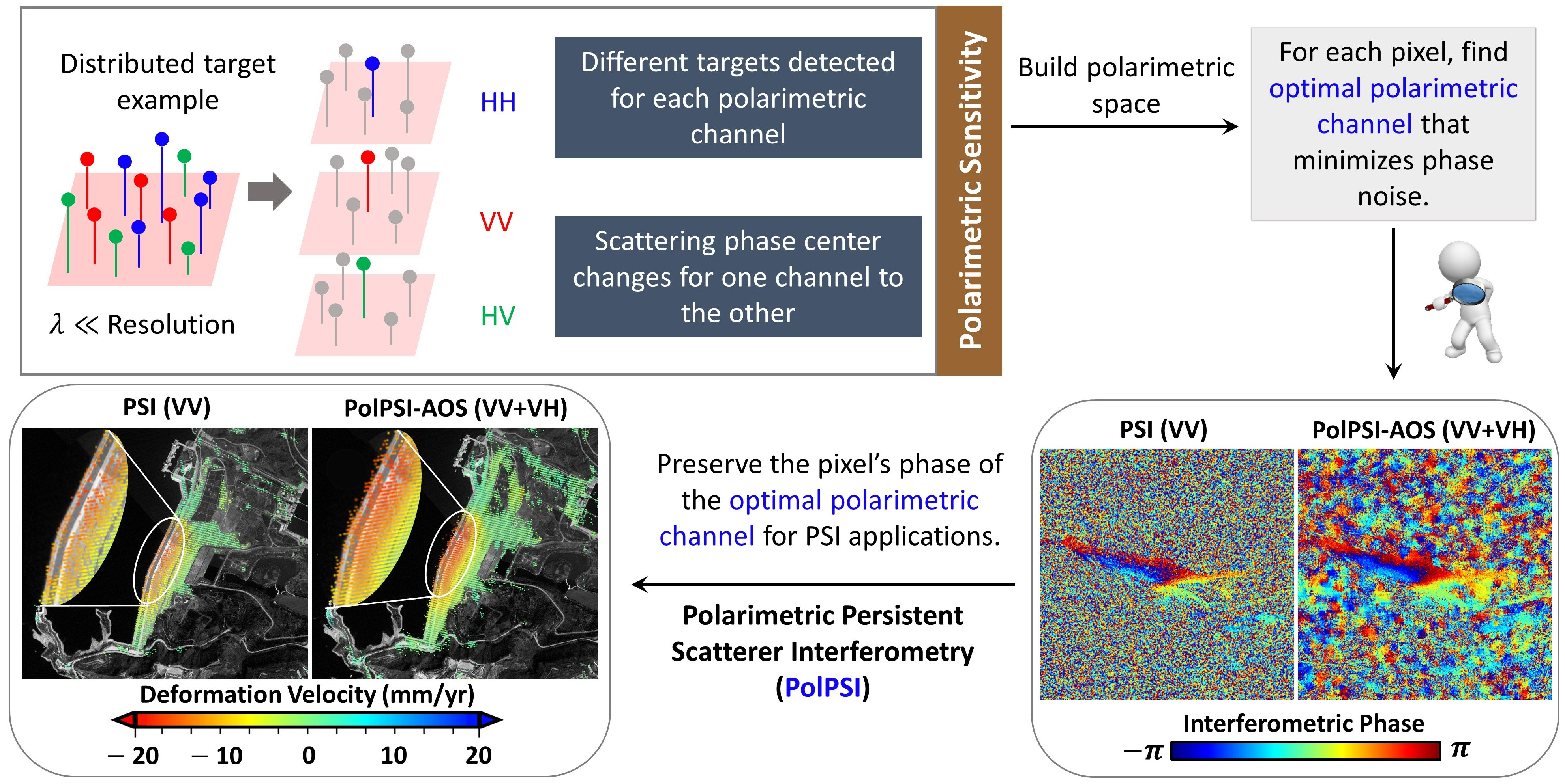
2.1. Polarimetric SAR Interferometry (PolInSAR)

The scattering matrix for one VV-VH Sentinel-1 PolSAR image can be expressed as
S = 0 S v h S v h S v v
where S v v and S v h are elements that correspond to the vertical and cross-polar channel, respectively. Under the Pauli basis, the scattering vector of (1) can be expressed as
k = [ S v v , 2 S v h ] T .
A pair of PolSAR images of the same area that are acquired from two slightly different look angles are required for PolInSAR [29,45]. Based on these two PolSAR images, the PolInSAR vector can be defined as
K = [ k 1 , k 2 ] T
where k 1 and k 2 are respectively the primary and secondary PolSAR images’ scattering vectors that can be obtained through (2).
Two polarimetric channels could generate two different interferograms separately. To obtain a single interferogram by combining these two channels, PolInSAR introduces two corresponding normalized complex projection vectors ω 1 and ω 2 , which can be expressed as
ω 1 , 2 = cos ( α ) sin ( α ) e j ψ , 0 α π / 2 π ψ < π
where α and ψ determine the scattering mechanism and phase relation of the scatterer, respectively [27,45]. ω 1 and ω 2 are usually regarded as Scattering Mechanisms (SMs), and the two original scattering vectors k 1 and k 2 are then projected onto their corresponding SMs with,
μ i = ω i · k i , i = 1 , 2
where † refers to the conjugate transpose. The obtained μ 1 and μ 2 are two complex scattering coefficients, which are analogous to single-polarization SAR images. Then, based on μ 1 and μ 2 , one interferogram can be generated with one PolSAR image pair [27,45]. In PolPSI applications, to avoid introducing artificial changes along time in scatterers’ phase centers that might be misinterpreted as the scatterers’ displacement, ω 1 and ω 2 are forced to be identical along the stack of images. In other words, for a particular dataset, a single projection vector ω (SM) is employed for all interferograms [29,30,45]. This constraint is usually named as Equal Scattering Mechanism (ESM) [46].
To obtain the interferogram stack with the overall lowest decorrelation (i.e., with the best phase quality) for PolPSI applications, every pixel should be polarimetric optimized via determining its best scattering mechanism ω . According to the different phase quality metrics employed for this polarimetric optimization, the most commonly used PolPSI algorithms can be categorized into three main categories. They are Polarimetric Persistent Scatterer Interferometry algorithms with amplitude dispersion index (i.e., D A in this study) optimization (PolPSI-ADI), with coherence optimization (PolPSI-COH), and with the adaptive optimization strategy (PolPSI-AOS), as introduced in Section 1.

2.2. Polarimetric Persistent Scatterer Interferometry with Amplitude Dispersion Index Optimization (PolPSI-ADI)

Amplitude dispersion index (i.e., D A in this study) is the mostly used phase quality metric for PS candidates’ optimization, in polarimetric case, it can be expressed as
D A = σ A m A = 1 | ω k | ¯ 1 N i = 1 N | ω k i | | ω k | ¯ 2
with
| ω k | ¯ = 1 N i = 1 N | ω k i |
where σ A and m A are the standard deviation and mean of the polarimetric synthesized SAR images’ amplitudes, N is the number of images, and the overline indicates the empirical mean value [29,30]. The polarimetric optimization of one pixel is to find the scattering mechanism ω that minimizes its D A (expressed by (6)), which is done through searching for the best parameters ( α , ψ ) as (4) indicates.
After the polarimetric optimization, for deterministic scatterers, the PolSAR image pair synthesized interferogram can be obtained through
I = μ 1 · μ 2 *
where * is the complex conjugate [29,30,45].

2.3. Polarimetric Persistent Scatterer Interferometry with Coherence Optimization (PolPSI-COH)

Different from the deterministic scatterers’ cases, the PolInSAR coherency matrix T 4 is used to characterize DS (distributed scatterer) pixels’ scatter behaviour, and for dual-pol Sentinel-1 PolSAR image it can be expressed as
T 4 = T 11 Ω 12 Ω 12 T 22
where T 11 and T 22 are the PolSAR coherency matrices and Ω 12 is the PolInSAR coherency matrix, and they are defined as
T 11 = E { k 1 k 1 } T 22 = E { k 2 k 2 } Ω 12 = E { k 1 k 2 }
where E is the expectation operator, which is usually implemented with a spatial average [27,45].
The polarimetric interferometric coherence γ ( ω ) is usually employed as the phase quality metric for DS pixels’ optimization. One interferogram, γ ( ω ) can be expressed as [27,45]
γ ( ω ) = | ω Ω 12 ω | ω T 11 ω ω T 22 ω .
For PolPSI applications, a stack of interferograms need to be optimization and, thus, the polarimetric mean coherence | γ ( ω ) | ¯ is employed, which can be calculated by
| γ ( ω ) | ¯ = 1 N k = 1 N | γ k ( ω ) |
where N is the number of interferograms. Similarly with the case of PolPSI-ADI, the optimization of a pixel is to search for the optimum scattering mechanism ω that maximizes its | γ ( ω ) | ¯ (expressed by (11) and (12)).
After the polarimetric optimization, based on the obtained optimum scattering mechanism ω , the vector interferogram for the optimized pixel can be generated with
I = E { μ 1 · μ 2 * } = E { ( ω k 1 ) ( ω k 2 ) } = ω E { k 1 k 2 } ω = ω Ω 12 ω .

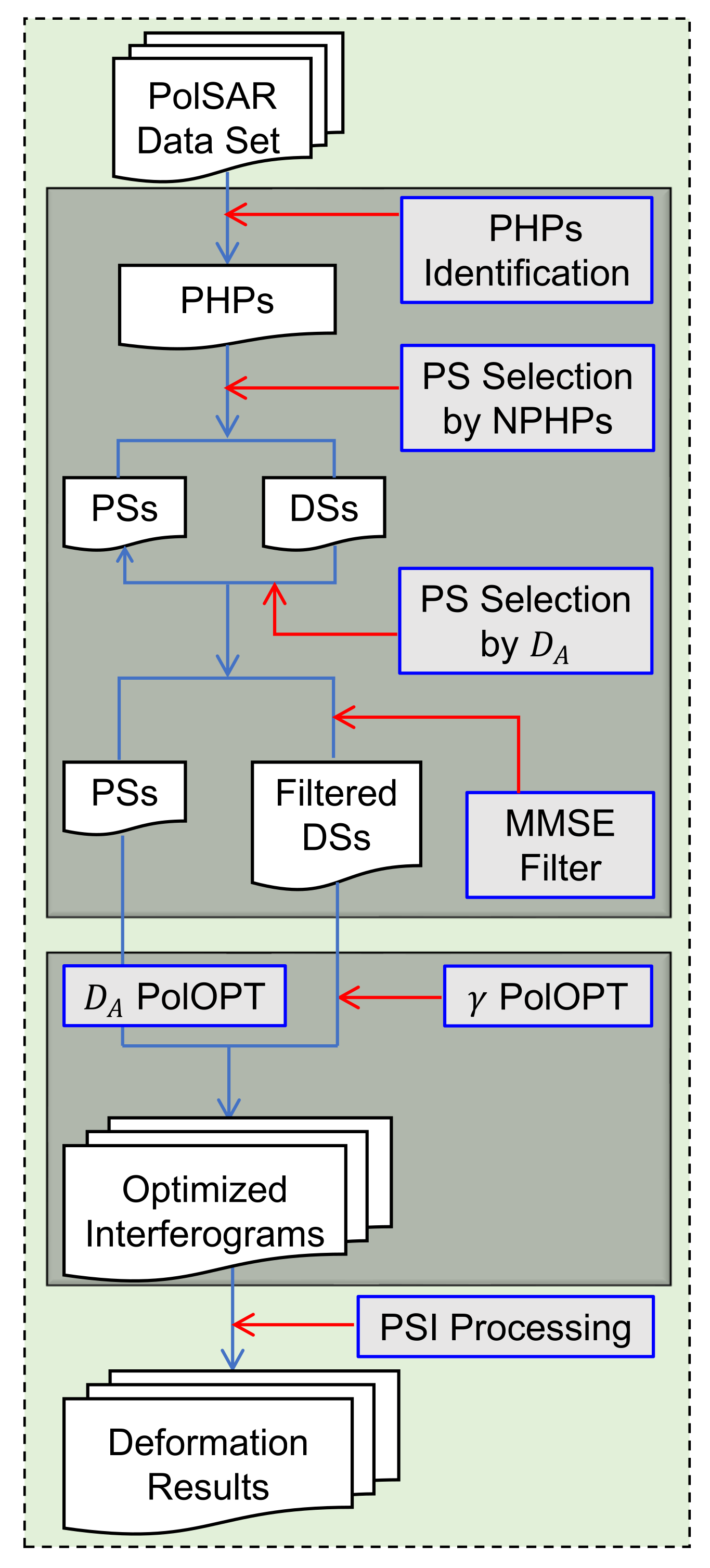
2.4. Polarimetric Persistent Scatterer Interferometry with the Adaptive Optimization Strategy (PolPSI-AOS)

The PolPSI-ADI and PolPSI-COH algorithms optimize all SAR pixels by one strategy, i.e., with D A or coherence optimization. However, as PS and DS pixels simultaneously exist in SAR images, more adaptive polarimetric optimization strategies are desired and have been proposed [31,37]. In this section, a PolPSI-AOS technique for the polarimetric optimization of Sentinel-1 interferograms is introduced. This PolPSI-AOS approach consists of two main procedures, i.e., the adaptive filtering of coherency matrix and polarimetric optimization. The flowchart of the introduced PolPSI-AOS is shown in Figure 1, and the details are described in the following two subsections.

2.4.1. Coherency Matrix Filtering

As Figure 1 shows, PolSAR pixels’ coherency matrix are adaptive filtered based on their polarimetric homogeneous pixels (PHPs). PHPs are those neighbouring pixels that with similar scattering mechanism. There are many techniques that can be used for each pixel’s PHPs identification, such as the PolSAR classification method in [37] and the likelihood ratio test approach in [31].
For Sentinel-1 data, considering its accuracy and efficiency, the fast statistically homogeneous pixels selection (FaSHP) technique [24] is modified to identify PHPs of each pixel. Firstly, by employing FaSHP, the homogeneous pixels (HPs) of each pixel of the VV and VH channel are separately identified (the window-size used is 15 × 15). Then, by combing pixels’ HPs of VV and VH channel, their PHPs are obtained. After that, by setting a threshold on the numbers of pixels’ PHPs, all the SAR pixels are categorized as PS and DS pixels, as Figure 1 shows. After testing a few threshold candidates over the test site, the threshold has been set to 20 for this study.
As Figure 1 shows, to avoid the misclassification of DS pixels, pixels’ best amplitude dispersion index D A B e s t are used to identify those PSs that have been misclassified as DSs, which is done by two steps. Firstly, D A B e s t values of all pixels are obtained by
D A B e s t = min { D A V V , D A V H }
where D A V V and D A V H are the ADI of VV and VH channel, which can be respectively calculated by the standard deviation and mean of the VV and VH channel SAR images’ amplitudes [2]. For those identified DSs whose D A B e s t values are smaller than 0.25 [2], they are recategorized as PSs.
As the SNR (signal-to-noise ratio) of PSs are usually high, to preserve images’ resolution, no filtering has been applied on them. To better preserve structures’ details, the minimum mean square error (MMSE) filter [27,47] is employed for the filtering of DSs’ coherency matrix (see Figure 1), which is given by
T filt = T mean + b ( T ori T mean )
where T filt and T ori are the filtered and original coherency matrices of the processing DS pixel, T mean is the mean of the recognized PHPs’ coherency matrices of this DS pixel. The filtering parameter b is used as a weighting factor to determine the degree of filtering, which is ranging from 0 to 1. The details of how to compute the weighting factor b can be found in [27,47]. It has to be noted that the introduced filter can be employed for both PolSAR and PolInSAR coherency matrices. In the PolPSI-AOS case, it is directly applied on the PolInSAR coherency matrix T 4 as (9) expressed.
After MMSE processing of T 4 through (15), the adaptive filtered interferograms corresponding to VV channel can be extracted from Ω 12 in the processed T 4 . Based on these MMSE filtered VV channel interferograms, the PSI processing can be applied for the ground deformation estimation. This method is referred as the MMSE method and it will be used for the comparison with PolPSI-AOS in Section 4.

2.4.2. Polarimetric Optimization

After adaptive filtering of T 4 , two different polarimetric optimization strategies are applied on PS and DS pixels, respectively. Specifically, PS pixels are optimized with D A (see (6)), which is similar with that in PolPSI-ADI, while DS pixels are optimized with | γ ( ω ) | ¯ (see (11) and (12)), which is based on the adaptively filtered T 4 rather than the spatial averaged ones in PolPSI-COH, as Figure 1 demonstrated.
For all the three kinds of PolPSI algorithms (i.e., PolPSI-ADI, PolPSI-COH, and PolPSI-AOS), the polarimetric optimization finds for each pixel the ω that minimizes its D A (for PS) or maximizes its | γ ( ω ) | ¯ (for DS). In this research, the Exhaustive Search Polarimetric Optimization (ESPO) method [30], which is an exhaustive search of the polarimetric space, has been used as it provides the best performance in interferometric phase optimization. The search step of the ESPO method is set as 3 for both D A and | γ ( ω ) | ¯ based optimizations.
After the polarimetric optimization, for PS or DS pixels, through (8) or (13), their optimized interferograms can be obtained, respectively. Then, based on these polarimetric optimized interferograms, the PSI processing can be carried out using the same algorithms as for the single-pol case, where StaMPS is employed in this study.

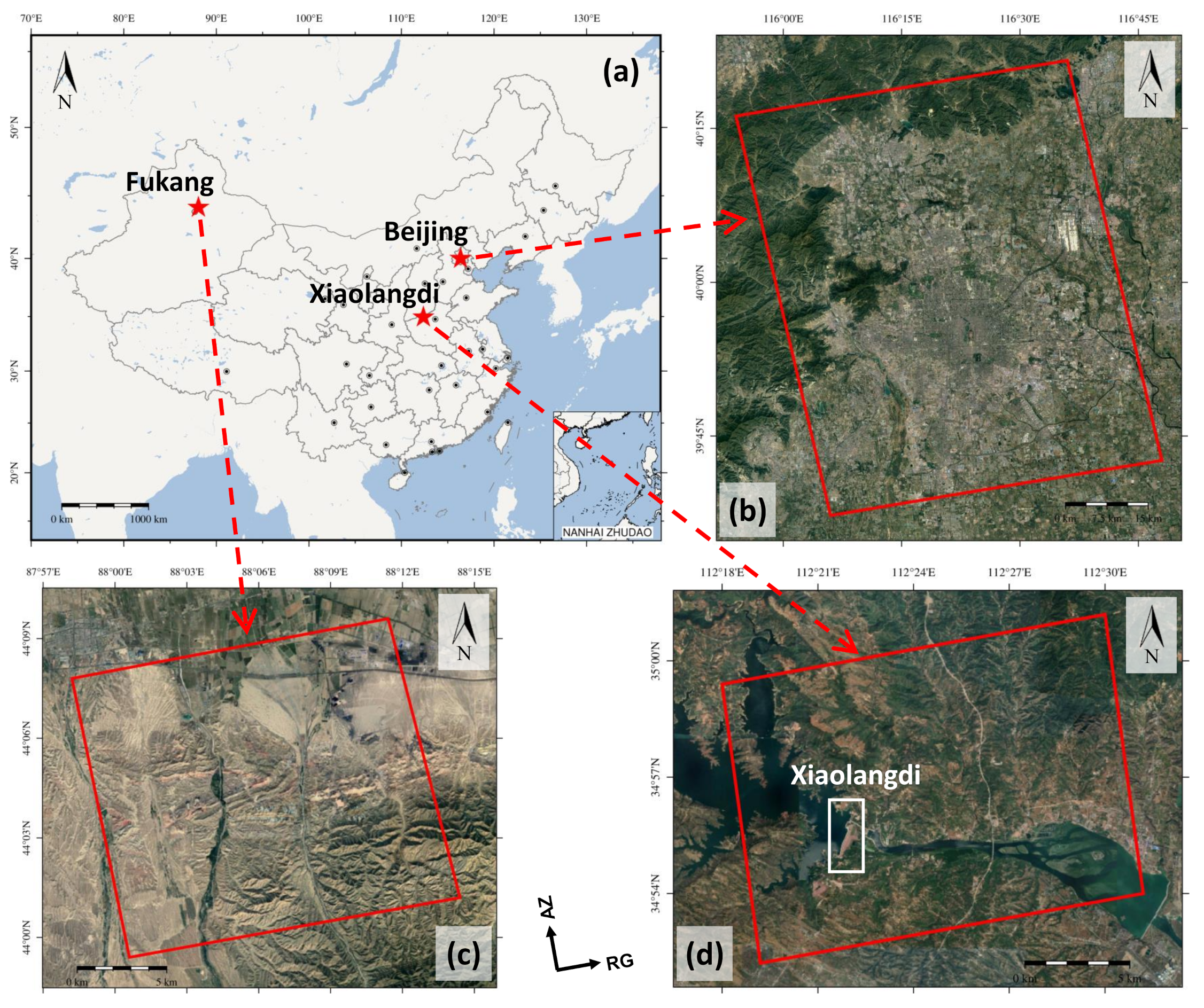
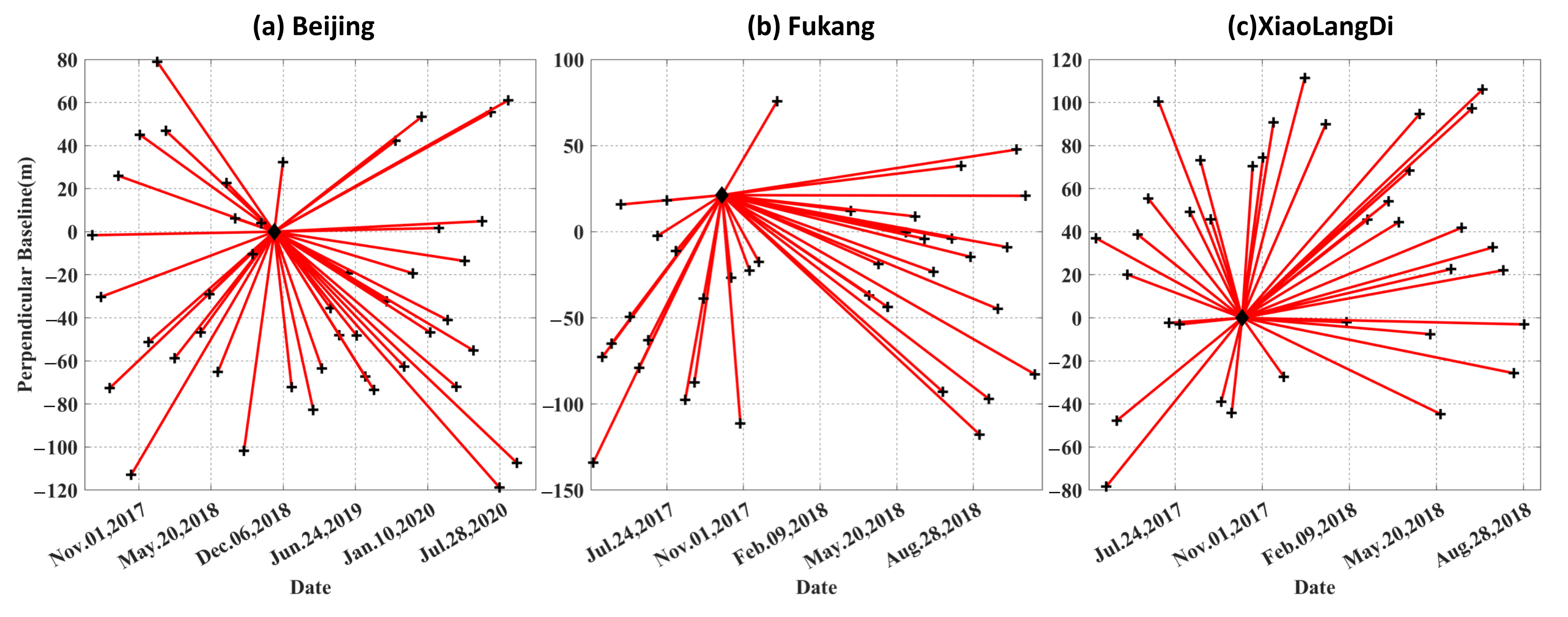
3. Data Sets and Test Sites

Dual-pol Sentinel-1 data sets over three test sites in China, which are with different land covers, are used to evaluate the performances of the three PolPSI approaches, respectively. The locations and corresponding optical images of the test sites are shown in Figure 2.
The first data set (for PolPSI-ADI evaluation) consists of 46 dual-pol Sentinel-1 images acquired from June 2017 to September 2020 over Beijing. Beijing is the capital city of China and has been suffering from ground deformation that is mainly caused by underground water extraction [48,49]. The processing has been applied over 5300 × 16 , 500 pixels in this study.
To assess the effectiveness of the PolPSI-COH technique, 40 dual-pol Sentinel-1 images (i.e., single complex), which were obtained from March 2017 to November 2018, over a bare land area of Fukang in Xinjing province has been employed. This test site has been affected by underground coal fire, where the coal fire related small ground deformation can be detected by PSI techniques. A section of the images with 1100 × 4000 pixels have been processed over this area.
To evaluate the performance of PolPSI-AOS, the area over the Yellow River XiaoLangDi dam of Henan province is selected as the third test site. Over this area, 38 dual-pol Sentinel-1 images acquired from April 2017 to August 2018 are employed for the deformation monitoring. XiaoLangDi dam is one of the largest dams in the world, and controls 92.3% of the total Yellow River Basin. The height of the dam is 154 m, and the length of the dam crest is about 1667 m. The maximum width of the dam bottom and the width of the dam crest are 864 m and 15 m, respectively.
For all the three data sets, the single reference method is used to obtain the interferograms, thus, 45, 39, and 37 interferograms have been generated (or synthesized by the PolPSI technique) for each case, respectively. The temporal and perpendicular baselines of the interferogram stacks over the three test sites are shown in Figure 3. Three Shuttle Radar Topography Mission (SRTM) digital elevation models (DEMs) are employed to simulate the tomography phases in interferograms for DInSAR (differential interferometric SAR) processing. The key parameters of the three data sets are listed in Table 1.

4. Results and Analysis

4.1. Results of the PolPSI-ADI
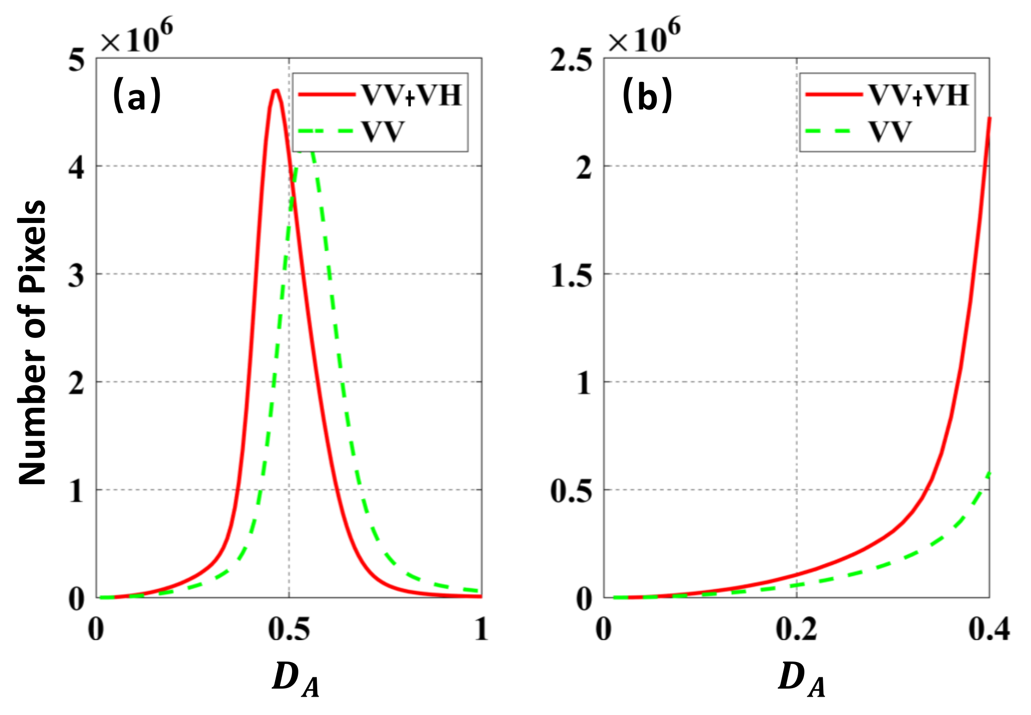
4.1.1. D A Optimization Results

The histograms of D A values derived by the VV channel and the PolPSI-ADI approach are shown in Figure 4. It can be observed from Figure 4 that, compared with the VV channel, there are more pixels with small D A values after polarimetric optimization through PolPSI-ADI. There is an offset between PolPSI-ADI (VV-VH) and VV related D A plots, which is due to the overall reduction of pixels’ D A values via polarization optimization of PolPSI-ADI. When D A is smaller than 0.4 it can be used for the approximation of pixels’ phase standard deviations [2]. Thus, it can be concluded from Figure 4b that after the polarimetric optimization the interferometric phase quality of pixels has been improved significantly.

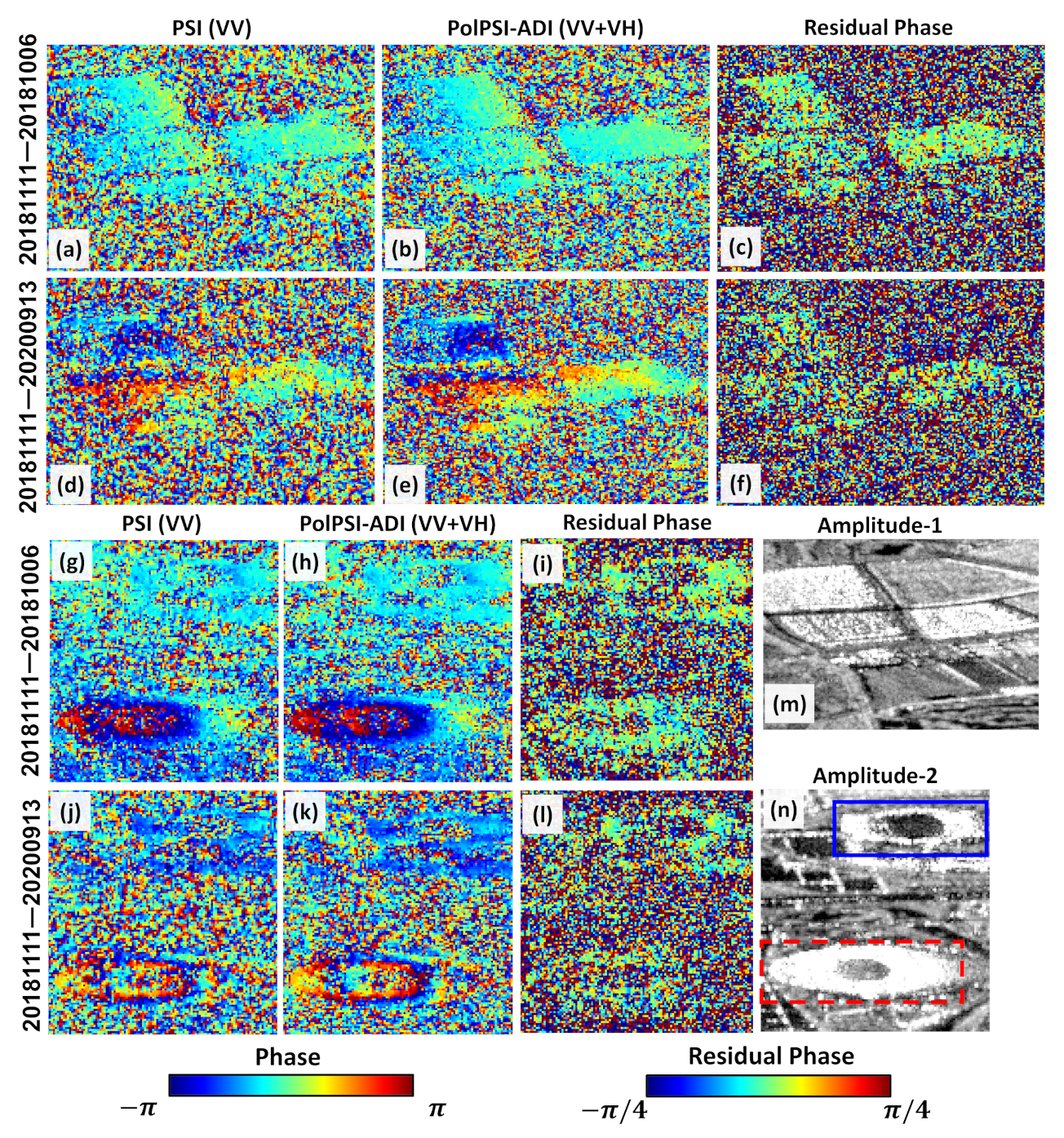
4.1.2. Performance on Interferograms’ Optimizations

The VV and PolPSI-ADI optimized interferograms (with VV and VH channels) over two subsections of Beijing are shown in Figure 5. These two subsections are chosen for the analysis because the different scattering mechanisms over these subareas (which makes interferograms noisy) and the noise of interferograms is supposed to be reduced by the optimization. The first subsection is over a group of buildings, whose amplitude image is as Figure 5m shows. Figure 5a,b is the interferogram pair (before and after optimization) with a shorter temporal baseline, and Figure 5d,e are the counterparts with a longer temporal baseline. Due to the orientation of buildings and mixture of different scattering mechanisms, the VV channel interferograms (see Figure 5a) are more noisy and the edges of man-made structures can be hardly seen. After the optimization via the PolPSI-ADI technique, the noise of interferograms have been reduced and the edges of the building groups are more clear (see Figure 5b). In addition, this area was suffering from subsidence and there are deformation fringes in the interferograms with the longer temporal baseline. However, in the VV channel interferogram (Figure 5d) the deformation fringes are masked by the noise and they are more clear after the polarimetric optimization (see Figure 5e). In addition, the corresponding two residual phase maps (i.e., PolPSI-ADI phase minus PSI phase) are plotted in Figure 5c,f. For effective phase optimization or filtering methods, the optimized pixels’ residual phase values are supposed to be noisy [50]. In the two residual phase maps (Figure 5c,f), noisy phases are observed on pixels with significant optimization effects, such as the edges of structures and along the deformation fringes. This indicates the good performance of the employed PolPSI-ADI method on interferometric phase optimization.
The second subsection is located around the China National Olympic Sports Center (see Figure 5n red rectangle) and the National Stadium (see Figure 5n blue rectangle). Affected by layover, mixing of various scattering mechanisms, and orientation of structures, the VV channel interferograms are blurred over the edge areas (see Figure 5g,j). After optimization, the phase noise of the interferogram is significantly reduced, and the corresponding phase contours (mainly due to DEM error) and edges of the two stadiums can be more clearly observed (see Figure 5h,k). Similar observations can be obtained from the corresponding residual phase maps (Figure 5i,l) as the first subsection, where pixels with phase quality improvement tend to with noisy residual phases (see the phase contour edge areas), proving the effectiveness of the phase optimization by PolPSI-ADI.

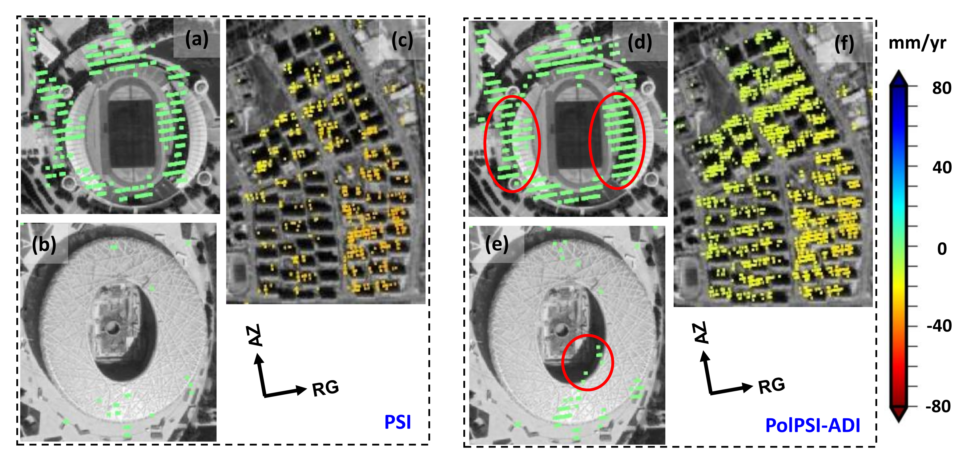
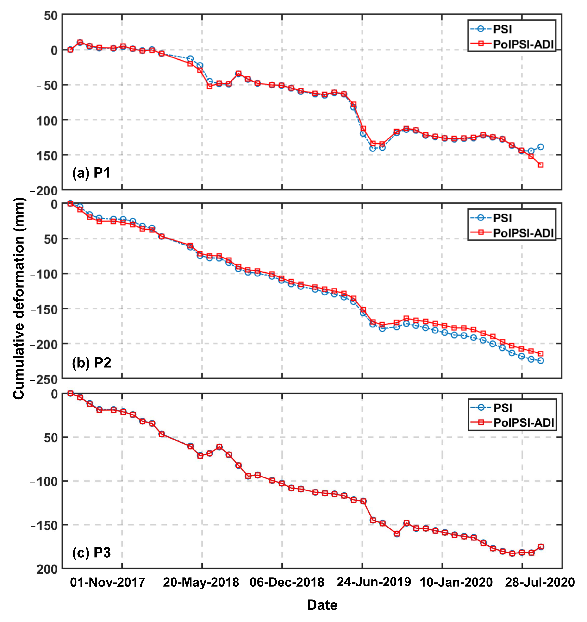
4.1.3. Ground Deformation Estimation

The VV and PolPSI-ADI optimized interferograms are employed for ground deformation estimation using the Stanford Method for Persistent Scatterers (StaMPS) [5,44]. To make a fair comparison, the same PSI processing parameters have been set for the two interferogram stacks, and the derived two ground deformation results are shown in Figure 6.
As Figure 6 shows, the obtained ground deformation patterns by the PSI and PolPSI-ADI algorithms are consistent with each other. The maximum and minimum deformation velocities obtained by PSI are respectively −76 mm/yr and 20 mm/yr, while the counterparts for PolPSI-ADI are −74 mm/yr and 20 mm/yr, respectively. The retrieved ground deformation magnitudes for the two approaches are also in good agreement with each other. There are three large subsidence bowls over the Beijing test site. The deformation areas are surrounding the center of Beijing city which is with no significant deformation during the observation period. As PolPSI-ADI has optimized the interferograms, it can obtain more PS pixels for ground deformation monitoring. The PS pixel density improvement achieved by PolPSI technique over Beijing test site is around 50% with respect to that of PSI. The obtained ground deformation details over the two subareas that are highlighted with white rectangles A and B in Figure 6a are shown in Figure 6c–f. The pixel density improvement achieved by PolPSI-ADI can be more clearly observed by comparing Figure 6c,e with Figure 6d,f. For instance, along the highway passing through subarea B (see the red dashed line in Figure 6e,f), PolPSI-ADI has obtained more qualified PS pixels for ground deformation monitoring than PSI.
To further illustrate this PS density improvement, the ground deformation over the three subsections (limited in Figure 6c,e with white rectangles C, D, and E), i.e., China National Olympic Sports Center (Figure 7a,d), the National Stadium (Figure 7b,e), and a group of departments (Figure 7c,f), are depicted in Figure 7. More details of deformation over the structures can be observed from the PolPSI-ADI obtained results. Moreover, as the red circles in Figure 7d,e indicate, the increased PS pixels tend to appear at the left side of the buildings, where layover usually occurs. This is because that for the VV channel interferograms, as layover happens over these areas, different scattering mechanisms tend to be mixed together, leading to decorrelations, thus, few qualified pixels can be employed for ground deformation monitoring. On the other hand, through the polarimetric optimization, the PolPSI-ADI technique can find the dominant scattering mechanisms of some pixels, thus, more qualified pixels can be used for PSI applications with respect to VV channel.
The numbers of pixels with different ground deformation velocity ranges retrieved by PSI and PolPSI-ADI have been given in Table 2. It can be found from Table 2 that, for all the listed deformation velocity ranges, there are pixel density improvements achieved by PolPSI-ADI with respect to PSI. This indicates the PolPSI-ADI technique is able to improve the ground deformation monitoring ability of PSI independent of the deformation magnitude over Beijing test site. Moreover, for relatively large subsidence range (−20 to −40 mm/yr), (−40 to −60 mm/yr), and (−60 to −80 mm/yr), the pixel density improvement is 61.95%, 32.10%, and 44.84%, respectively. This means that more areas with relative large ground deformation can be detected by using PolPSI-ADI than PSI. Specifically, the size of this extra detected significant subsidence area is around 838.61 hm 2 as Table 2 indicates.
The deformation time-series of three pixels P1, P2, and P3 (see the three white circle in Figure 6a), over three deformation centers are shown in Figure 8. No obvious difference has been observed for the PSI and PolPSI-ADI obtained results. Except some variations that may be caused by the rebound of the groundwater [48,49], the three pixels had nearly linear subsidence trends during the observing period. Specifically, the maximum cumulative subsidence for the three pixels is respectively around 150 mm, 220 mm, and 180 mm, which indicates that there are some subareas surrounding the Beijing central district that are still suffering from significant subsidence.

4.2. Results of the PolPSI-COH

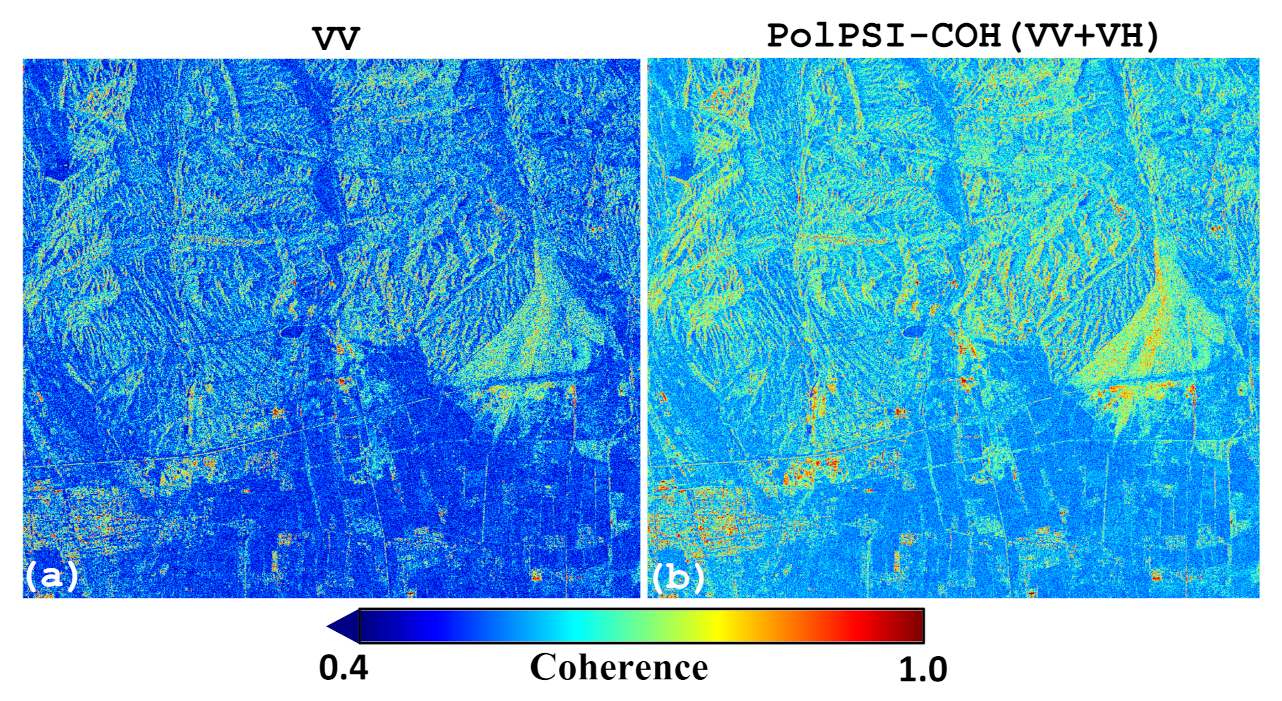
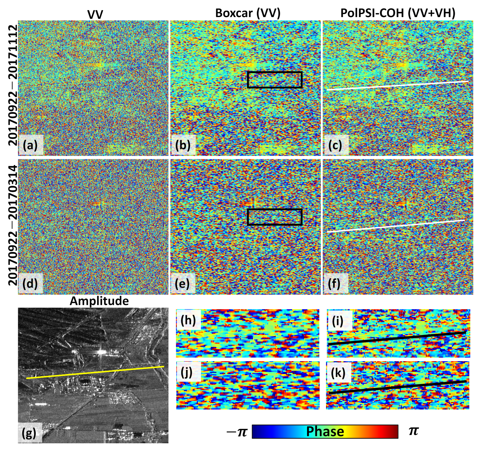
4.2.1. Coherence and Interferograms’ Optimization Results

The window size of 5 × 5 is used for the polarimetric optimization with coherence over the Fukang area. The temporal average coherence of VV channel interferograms (estimated with 5 × 5 boxcar approach) and the optimized one is shown in Figure 9a,b, respectively. It can be observed from the figure that after the polarimetric optimization, the coherence has been improved significantly. This indicates that the PolPSI-COH technique can improve the phase quality of interferograms.
To compare the polarimetric optimization effect on the interferograms, interferograms over a subsection of VV channel, the boxcar, and the PolPSI-COH approach are shown in Figure 10. Both the boxcar (see Figure 10b,e) and PolPSI-COH (see Figure 10c,f) method can improve the interferometric phase quality as the noise has been reduced in the processed interferograms with respect to VV channel ones (see Figure 10a,d). However, PolPSI-COH can better preserve edges of structures than the boxcar approach. For instance, there is a left to right road over the subsection (see the lines in Figure 10c,f,g), after processing by boxcar it can be hardly observed. On the other hand, this road can be distinguished from the background noisy phases in the PolPSI-COH obtained results (see Figure 10c,f,i,k). This is because after boxcar processing the neighbouring pixels are averaged, and details are lost. However, the polarimetric optimization can extract the dominant scattering mechanisms from the mixed ones within the averaged pixels, thus, more details can be retrieved than from the boxcar approach.

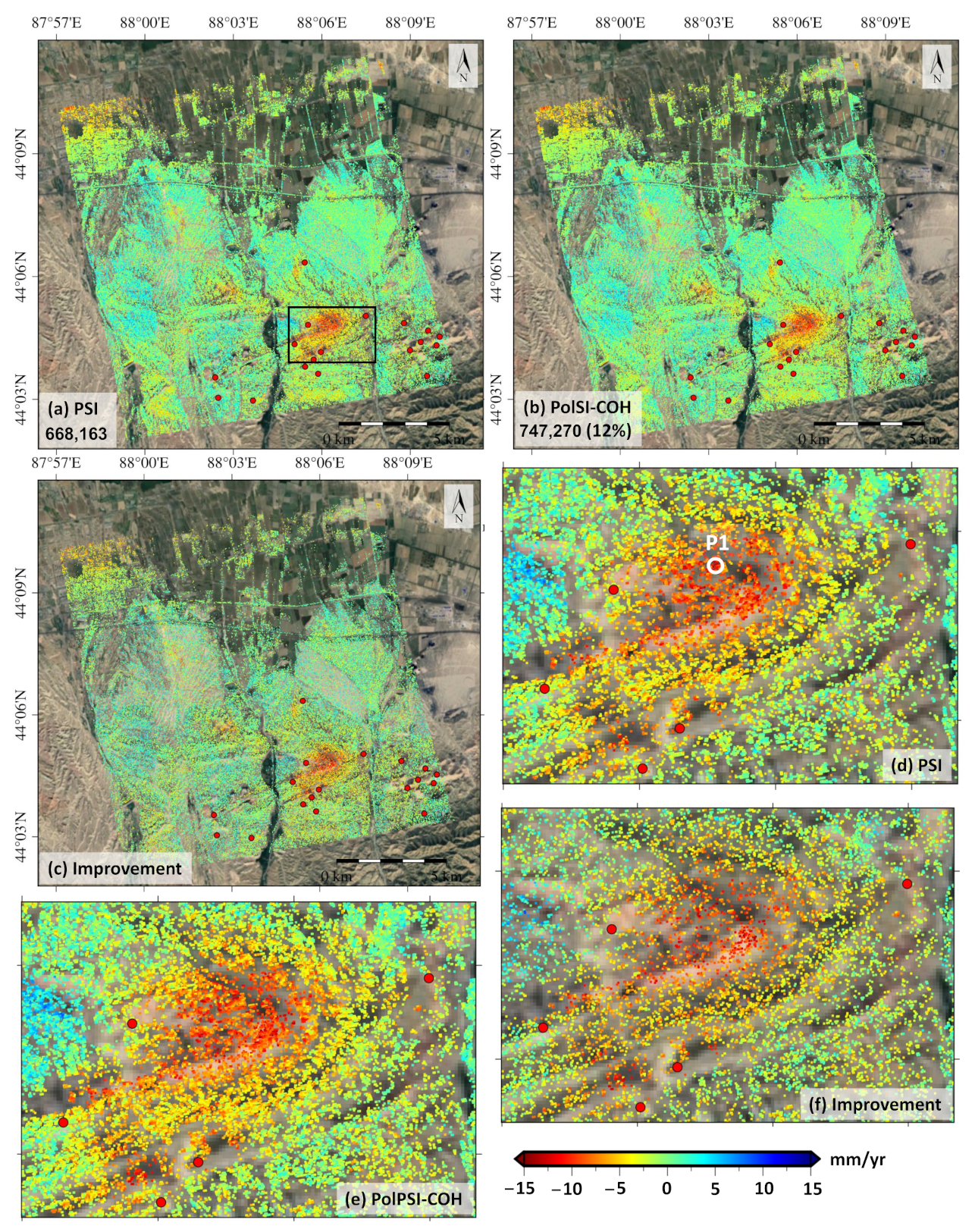
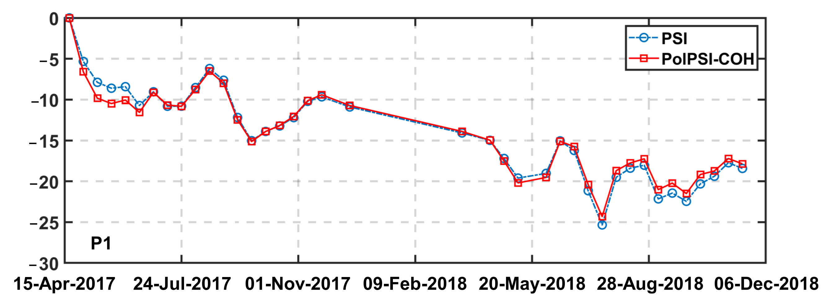
4.2.2. Ground Deformation Estimation

The Boxcar and PolPSI-COH method processed interferograms are used for ground deformation retrieved over the Fukang area. To make a fair comparison, for both PSI processing the StaMPS processing parameters are set as the same values. The two approaches that obtained results are shown in Figure 11.
The two retrieved ground deformation pattens are very similar (see Figure 11a,b), with the maximum and minimum deformation velocities as 9 mm/yr and −17 mm/yr for both method results. The most significant deformation areas are located over the coal fire areas, as the black rectangle in Figure 11a indicates. In this subsection, the field survey coal fire points (red filled dots) are distributed around the edge of the subsidence bowl. This is because that the geological surveyor cannot go deep into the coal fire area for safety considerations. It can be observed from Figure 11 that there are some coal fire points that have no deformation. This could be caused by the corresponding coal fires being deeper underground or at their earlier stages, thus, they could not cause significant deformation on the ground during the observation. On the other hand, there are some subsidence areas where there are no coal fire points. This is due to these subsidence being caused by human activities (e.g., mining) rather than underground coal fires.
More pixels can be obtained by PolPSI-COH for ground deformation monitoring than PSI, and this improvement on pixels’ density is 12% over the Fukang area. Figure 11c demonstrates this improvement on pixel density achieved by PolPSI-COH with respect to PSI over the whole area. It can be observed from Figure 11c that this improvement is more significant in areas with relatively high coherence, which indicates the reliability of the added deformation measurement pixels. To further demonstrate the pixel density improvement, the retrieved ground deformation results by the PSI and PolPSI-COH methods over the Laobata coal fire area is shown in Figure 11d,e. More deformation details can be observed from the Pol-COH derived result, which benefited from the extra pixels (see Figure 11f) obtained by PolPSI-COH with respect to that of PSI. These more detailed ground deformation monitoring results can be more useful to study the coal fire related ground displacement phenomena and the related coal fire extinction projects.
The numbers of pixels with different ground deformation velocity ranges obtained by PSI and PolPSI-COH over Fukang test site are given in Table 3. PolPSI-COH is able to achieve higher pixel density with respect to that of PSI for pixels with all the three detected velocity ranges. Moreover, among the three deformation velocity categories, this improvement is most significant for the large subsidence range (i.e., −10 to −15 mm/yr). This indicates that the PolPSI-COH technique has better performance than PSI in large deformation monitoring over the Fukang area, which can be an advantage for the detection of coal fire areas. If areas with the subsidence rate greater than −10 mm/yr are classified as suspected coal fire areas, as Table 3 shows, around 1.96 hm 2 extra coal fire areas (23.70% improvement) can be detected by PolPSI-COH comparing PSI.
The deformation time-series of a pixel within the Laobata coal fire area (see the white circle P1 in Figure 11d) is shown in Figure 12. As the figure shows, the selected pixel was suffering from nonlinear deformation, which is with an overall subsidence trend, and the maximum cumulative subsidence is around 25 mm. Due to the shortage of more coal fire related information, the cause of this nonlinear deformation trend could not be analyzed in this study.

4.3. Results of the PolPSI-AOS

To test the performance of PolPSI-AOS, the VV channel results and the MMSE method processed results are employed for the comparison. It should be noted that the MMSE approach is actually a DS-InSAR method. It takes use of the information contained in the dual-pol SAR data for the VV channel interferograms’ adaptive filtering. Then, the filtered VV channel interferograms and the optimized interferograms (VV+VH) are used for the PSI processing for the MMSE and PolPSI-AOS technique, respectively. To make fair comparisons, the StaMPS PSI processing parameters are the same for the three methods (i.e., PSI, MMSE, and PolPSI-AOS).

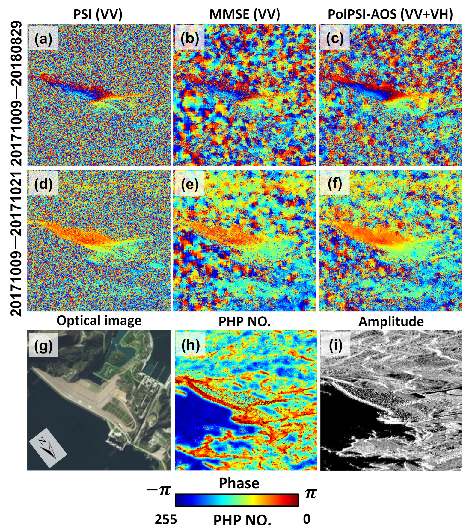
4.3.1. Performance on Interferograms’ Optimizations

The VV channel, MMSE, and PolPSI-AOS obtained interferograms of two temporal baselines over the XiaoLangDi dam are depicted in Figure 13a–f. The number of the identified PHPs for each pixel over the subsection is shown in Figure 13h. By comparing with the corresponding optical (Figure 13g) and amplitude images (Figure 13i), it can be found that large numbers of PHPs appeared at the homogeneous areas like the sea and mountain areas, whereas small values are located at the heterogeneous areas like the edges of the dam. This demonstrates the reliability of the PHPs’ identification result.
The MMSE method can reduce the interferograms’ phase noise and preserve details of structures compared with the VV channel interferograms. This is due to its adaptive filtering strategy, where PS pixels are with no processing and DS pixels are adaptive averaged together with their PHPs. The PolPSI-AOS approach firstly adapts filter interferograms the same as the MMSE method, and after that the filtered interferograms are further polarimetric optimized by using the dual-pol data. Thus, compared with the MMSE results, PolPSI-AOS processed interferograms are with better phase quality. For instance, there are less noisy pixels over the dam in PolPSI-AOS results (see Figure 13 c,f) than that of MMSE results (see Figure 13b,e).

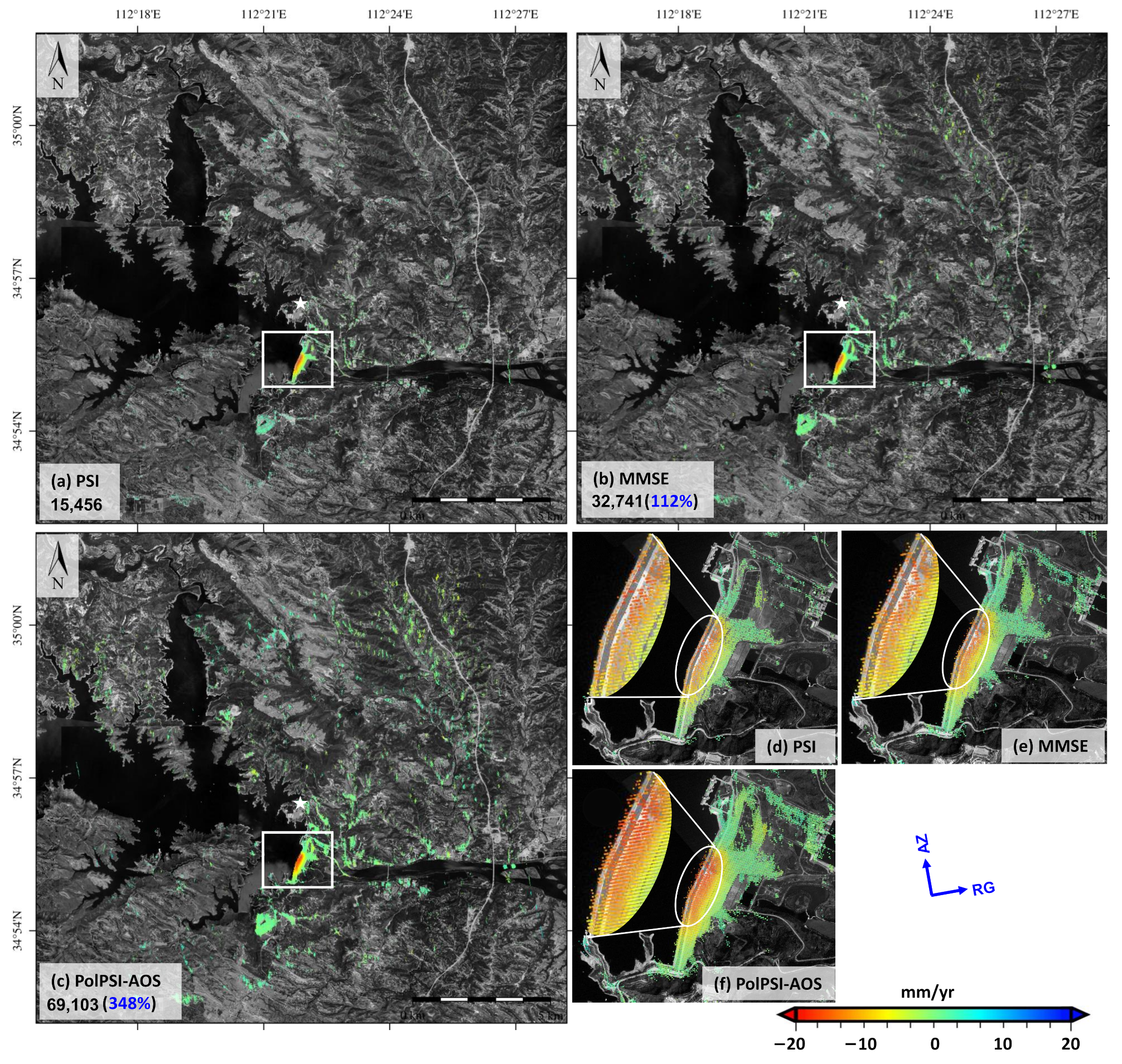
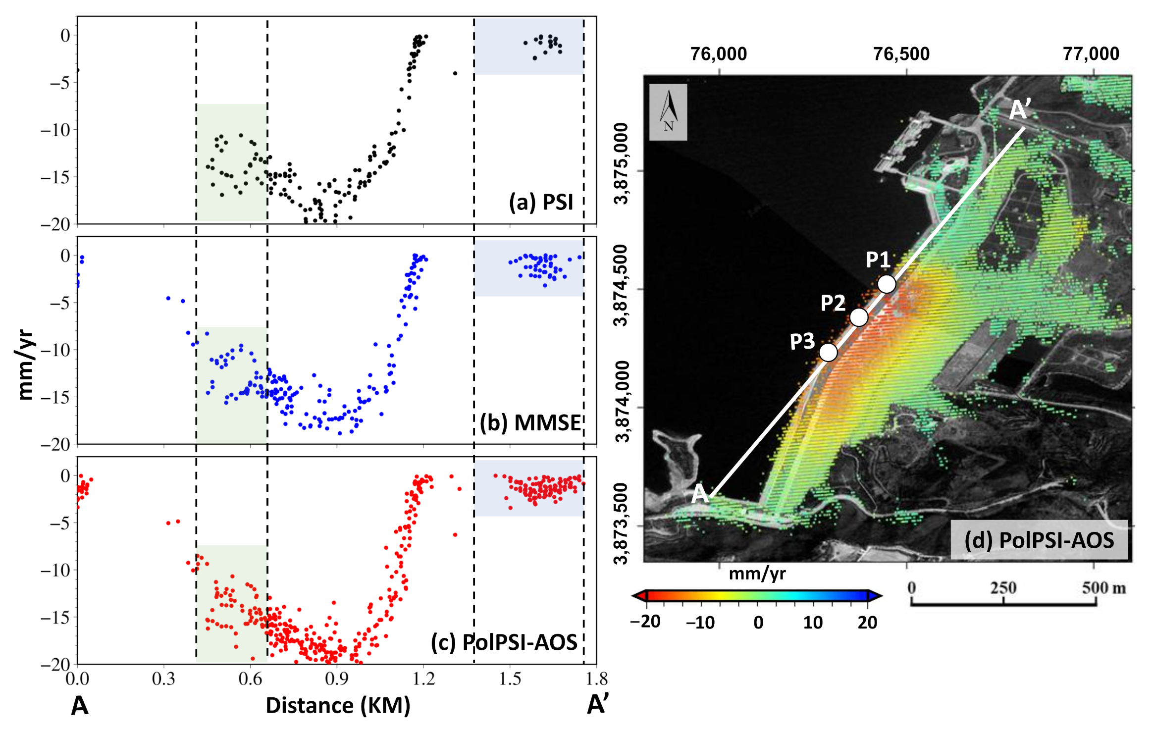
4.3.2. Ground Deformation Estimation

The three approaches (i.e., PSI, MMSE, and PolPSI-AOS) that retrieved ground deformation velocity over the XiaoLangDi dam area are shown in Figure 14. The detected deformation patterns and the retrieved deformation magnitudes by the three techniques are very similar, where significant deformation is observed over the dam. Specifically, the minimum and maximum deformation velocities retrieved by PSI, MMSE, and PolPSI-AOS are (−20 mm/yr, 8 mm/yr), (−19 mm/yr, 13 mm/yr), and (−20 mm/yr, 11 mm/yr), respectively. Mainly affected by the vegetations (temporal decorrelations), very sparse pixels have been selected over mountainous areas, where the PolPSI-AOS has the best performance. On the other hand, all the three methods are able to obtain denser pixels around the dam area. In total, 15,456, 32,741, and 69,103 final pixels have been obtained by the PSI, MMSE, and PolPSI-AOS, respectively. Both MMSE and PolPSI-AOS are able to obtain more pixels than PSI, and their corresponding improvement with respect to PSI is 112% and 348%, respectively.
The acquired ground deformation close-up over the dam of the three methods are shown in Figure 14d,e,f. The main body of the dam shows an obvious law of large deformation in the middle and stable at both ends, which is in line with the general law of dam deformation. As more pixels have been obtained by PolPSI-AOS, more details of the dam deformation can be found in its result.
The PSI and PolPSI-AOS obtained ground deformation monitoring pixels are categorized into three ranges based on their deformation velocities, the numbers of pixels of all the categories are listed in Table 4. Similar with the Beijing and Fukang test sites cases, pixel density improvements have been achieved by PolPSI-AOS for all the deformation velocity ranges with respect to PSI. As a result, more pixels (additional areas as Table 4 last column shows) with significant deformation over the dam can be detected by using PolPSI-AOS rather than PSI.
To further demonstrate the above points, the selected pixels by PSI, MMSE, and PolPSI-AOS along with a profile (see the white line from A to A’ in Figure 15d) passing through the dam front are depicted in Figure 15a–c, respectively. As the green and blue filled rectangles highlight, the PolPSI-AOS performs best in pixel density, which means more details of the dam’s deformation can be captured by employing it than the other two techniques.
To analysis the relationship between the dam deformation and water level of the reservoir basin, deformation time-series of three pixels (i.e., P1, P2, and P3) along the profile in Figure 15d have been depicted together with the corresponding water level in Figure 16. It can be observed from Figure 16 that the three methods obtained time-series are very similar in general. In addition, the time-series deformation is negatively correlated with the water level for all the three points. As the reservoir basin water level periodically changes, the dam is supposed to with periodic deformation trend. Specifically, when the water level increases the dam move away from the satellite (i.e., the cumulative deformation decreases) and vice versa. Moreover, the local maximum values of water level are always corresponds to the local minimum values of the cumulative deformation and vice versa (see the brown and blue filled rectangles highlighted sections in Figure 16). This indicates that the deformation of the dam is mainly caused by the change of the reservoir basin water level, and it can also prove the effectiveness of the employed three deformation monitoring methods.

5. Discussion

The computation time and different characteristics of the three types of PolPSI techniques is discussed in this section. The results have demonstrated that the PolPSI techniques perform better than the corresponding PSI techniques in ground deformation monitoring over the three test areas. However, more computational cost has to be paid for the PolPSI techniques as they optimize interferograms through searching for the optimum scattering mechanism for each pixel. Pixels’ polarimetric optimization time for the three employed PolPSI techniques have been listed in Table 5.
The implementation is in Matlab R2016b, and the three processings have been carried out on a workstation equipped with an 8 core Intel (R) Xeon (R) Gold 5222 processor and 256 GB of RAM. It has to be noted that only one CPU has been used for each processing. In other words, no parallel processing strategy has been employed. The searching step of the optimum parameters (i.e., α and ψ ) in the ESPO method [30] is set as 3 for all the three PolPSI techniques.
It can be found from Table 5 that the PolPSI-AOS is with the highest computation burden for per million pixels’ optimization. This is because it filtered all the pixels by the MMSE filter before optimizations, thus, it takes around 11.3 h to optimize per million pixels. On the other hand, the PolPSI-ADI approach is much faster than the other two where only around 1.1 h is required for per million pixels’ polarimetric optimization. This is due to the calculation of D A (see (6)), which is much easier than that of | γ ( ω ) | ¯ (see (11) and (12)). Nevertheless, for the Beijing areas’ polarimetric optimization with D A , it takes around 100 h.
It can be observed from Table 5 that the long computation time may limit the use of PolPSI techniques for large areas’ ground deformation monitoring, especially for the PolPSI-AOS method. In general, we can address this drawback of PolPSI via two approaches. On the one hand, more powerful workstations or even servers can be used to accelerate pixels’ polarimetric optimization speed. Or, by the other way, parallel computation strategies can be employed. On the other hand, more efficient phase polarimetric optimization methods (e.g., CMD method [36]) instead of ESPO [28] can be used to reduce the computation burden. However, it worth to note that it is always a trade-off between the optimization effectiveness and efficiency.
Different PolPSI techniques should be used for the ground deformation monitoring over areas with different land covers. Specifically, for city areas, where there are abundant PS pixels, PolPSI-ADI is the first choice as it is fast and it can preserve SAR image resolutions. Thus, more details of deformation could be retrieved. However, for rural areas, where DS pixels are the majority, the PolPSI-COH or PolPSI-AOS approaches should be employed. As Table 5 indicates, the improvement achieved by PolPSI-COH is insignificant over the Fukang area. This is mainly due to the multi-look processing applied on the medium resolution Sentinel-1 SAR images, where more scattering mechanisms have been averaged within one resolution cell, resulting the failure of separating the dominant one for PSI applications. Therefore, the PolPSI-AOS method is suggested for the ground deformation monitoring in rural areas. It is able to adaptively process PS and DS pixels. Thus, details can be preserved for PS pixels, and DS pixels can be adaptively filtered without mixing many different scattering mechanisms, thus, they could be better optimized than using PolPSI-COH.

6. Conclusions

The three most commonly used PolPSI techniques with Sentinel-1 dual-pol (i.e., VV and VH) SAR images have been introduced and their effectiveness and suitability have been evaluated over three test sites within China in this study. The results obtained have allowed us to obtain the following main conclusions:
(1)
All the three types of PolPSI techniques are able to improve interferograms’ phase qualities through the polarimetric optimization with VV and VH Sentinel-1 images. After the polarimetric optimizations, edges of structures become more clear and phase noises are reduced.
(2)
The improvement in density of final deformation monitoring pixels with respect to conventional PSI techniques is 50 % , 12 % , and 348 % for PolPSI-ADI, PolPSI-COH, and PolPSI-AOS, respectively. The PolPSI-AOS algorithm is with the best performance among the three, which also has the longest computation time.
(3)
PolPSI-ADI is the most efficient (fast) algorithm, and it is the first choice when applying to the areas with abundant PS pixels. PolPSI-COH is not suggested to be applied on Sentinel-1 PolSAR images, because it has small improvement and relatively long computation time with respect to conventional PSI method as the results indicate. PolPSI-AOS is suggested to be applied for areas where DS pixels have to be employed to retrieve ground deformation with Sentinel-1 PolSAR images.
From this study, it can be concluded that it is worth processing the two channels (i.e., VV and VH) of the Sentinel-1 data by applying the PolPSI techniques, since interferograms’ quality can be improved and more detailed and reliable deformation maps can be obtained than just using VV channel data. However, the better results achieved by PolPSI techniques are at the cost of much higher computation burdens than conventional PSI methods. This problem can be partially solved by taking parallel processing strategies or choosing existing more efficient polarimetric optimization methods like the CMD. On the other hand, to solve the bottleneck of PolPSI algorithms, more polarimetric optimization methods with shorter processing time and satisfactory optimization performance should be developed, which is also our future research focus.

Author Contributions

Conceptualization, F.Z. and Y.W.; methodology, F.Z., H.F. (Han Feng) and L.Z.; validation, F.Z., T.W., S.Y. and D.X.; results analysis, H.F. (Han Feng), S.Y. and D.X.; writing—review and editing, F.Z. and T.W.; visualization, L.Z. and T.W.; supervision, S.Y., H.F. (Hongdong Fan) and Y.W.; project administration, Y.W. All authors have read and agreed to the published version of the manuscript.

Funding

This work has been supported in part by the National Natural Science Foundation of China (Grant 42004011, 41874044), in part by the China Postdoctoral Science Foundation (Grant No. 2020M671646), in part by the First-class research projects of Yellow River Engineering Consulting Co.,Ltd. (Grant No. 2021KY055), and in part by the Priority Academic Program Development (PAPD) of Jiangsu Higher Education Institutions (Science and Technology of Surveying and Mapping).

Institutional Review Board Statement

Not applicable.

Informed Consent Statement

Not applicable.

Data Availability Statement

The Sentinel-1A data used in this study are provided by the European Space Agency (ESA), https://scihub.copernicus.eu/dhus/#/home (accessed on 1 December 2021); POD Precise Orbit Ephemerides used in this study are provided by the ESA, https://scihub.copernicus.eu/gnss/#/home (accessed on 1 December 2021); and the SRTM DEM is freely downloaded from the website https://earthexplorer.usgs.gov/ (accessed on 1 December 2021).

Acknowledgments

The Sentinel-1 data are provided by the European Space Agency. Some figures were prepared using the public domain GMT software (Wessel and Smith, 1998). Optical images provided by GoogleEarth.

Conflicts of Interest

The authors declare no conflict of interest.

References

  1. Ferretti, A.; Prati, C.; Rocca, F. Nonlinear subsidence rate estimation using permanent scatterers in differential SAR interferometry. IEEE Trans. Geosci. Remote Sens. 2000, 38, 2202–2212. [Google Scholar] [CrossRef] [Green Version]
  2. Ferretti, A.; Prati, C.; Rocca, F. Permanent scatterers in SAR interferometry. IEEE Trans. Geosci. Remote Sens. 2001, 39, 8–20. [Google Scholar] [CrossRef]
  3. Berardino, P.; Fornaro, G.; Lanari, R.; Sansosti, E. A new algorithm for surface deformation monitoring based on small baseline differential SAR interferograms. IEEE Trans. Geosci. Remote Sens. 2002, 40, 2375–2383. [Google Scholar] [CrossRef] [Green Version]
  4. Mora, O.; Mallorqui, J.J.; Broquetas, A. Linear and nonlinear terrain deformation maps from a reduced set of interferometric SAR images. IEEE Trans. Geosci. Remote Sens. 2003, 41, 2243–2253. [Google Scholar] [CrossRef]
  5. Hooper, A.; Zebker, H.; Segall, P.; Kampes, B. A new method for measuring deformation on volcanoes and other natural terrains using InSAR persistent scatterers. Geophys. Res. Lett. 2004, 31, L23611. [Google Scholar] [CrossRef]
  6. Blanco-Sanchez, P.; Mallorquí, J.J.; Duque, S.; Monells, D. The coherent pixels technique (CPT): An advanced DInSAR technique for nonlinear deformation monitoring. Pure Appl. Geophys. 2008, 165, 1167–1193. [Google Scholar] [CrossRef]
  7. Iglesias, R.; Mallorqui, J.J.; Monells, D.; López-Martínez, C.; Fabregas, X.; Aguasca, A.; Gili, J.A.; Corominas, J. PSI deformation map retrieval by means of temporal sublook coherence on reduced sets of SAR images. Remote Sens. 2015, 7, 530–563. [Google Scholar] [CrossRef] [Green Version]
  8. Zhao, F.; Mallorqui, J.J. A Temporal Phase Coherence Estimation Algorithm and Its Application on DInSAR Pixel Selection. IEEE Trans. Geosci. Remote Sens. 2019, 57, 8350–8361. [Google Scholar] [CrossRef] [Green Version]
  9. Ferretti, A.; Savio, G.; Barzaghi, R.; Borghi, A.; Musazzi, S.; Novali, F.; Prati, C.; Rocca, F. Submillimeter accuracy of InSAR time series: Experimental validation. IEEE Trans. Geosci. Remote Sens. 2007, 45, 1142–1153. [Google Scholar] [CrossRef]
  10. Casu, F.; Manzo, M.; Lanari, R. A quantitative assessment of the SBAS algorithm performance for surface deformation retrieval from DInSAR data. Remote Sens. Environ. 2006, 102, 195–210. [Google Scholar] [CrossRef]
  11. Zhao, F.; Wang, Y.; Yan, S.; Lin, L. Reconstructing the vertical component of ground deformation from ascending ALOS and descending ENVISAT datasets—A case study in the Cangzhou area of China. Can. J. Remote Sens. 2016, 42, 147–160. [Google Scholar] [CrossRef]
  12. Cigna, F.; Tapete, D. Present-day land subsidence rates, surface faulting hazard and risk in Mexico City with 2014–2020 Sentinel-1 IW InSAR. Remote Sens. Environ. 2021, 253, 112161. [Google Scholar] [CrossRef]
  13. Fan, H.; Lu, L.; Yao, Y. Method combining probability integration model and a small baseline subset for time series monitoring of mining subsidence. Remote Sens. 2018, 10, 1444. [Google Scholar] [CrossRef] [Green Version]
  14. Du, S.; Mallorqui, J.J.; Fan, H.; Zheng, M. Improving PSI Processing of Mining Induced Large Deformations with External Models. Remote Sens. 2020, 12, 3145. [Google Scholar] [CrossRef]
  15. Du, Y.; Yan, S.; Yang, H.; Jiang, J.; Zhao, F. Investigation of deformation patterns by DS-InSAR in a coal resource-exhausted region with Spaceborne SAR imagery. J. Asian Earth Sci. X 2021, 5, 100049. [Google Scholar] [CrossRef]
  16. Liu, F.; Elliott, J.; Craig, T.; Hooper, A.; Wright, T. Improving the Resolving Power of InSAR for Earthquakes Using Time Series: A Case Study in Iran. Geophys. Res. Lett. 2021, 48, e2021GL093043. [Google Scholar] [CrossRef]
  17. Fernández, J.; Escayo, J.; Hu, Z.; Camacho, A.G.; Samsonov, S.V.; Prieto, J.F.; Tiampo, K.F.; Palano, M.; Mallorquí, J.J.; Ancochea, E. Detection of volcanic unrest onset in La Palma, Canary Islands, evolution and implications. Sci. Rep. 2021, 11, 2540. [Google Scholar] [CrossRef]
  18. Zhao, F.; Mallorqui, J.J.; Iglesias, R.; Gili, J.; Corominas, J. Landslide Monitoring Using Multi-Temporal SAR Interferometry with Advanced Persistent Scatterers Identification Methods and Super High-Spatial Resolution TerraSAR-X Images. Remote Sens. 2018, 10, 921. [Google Scholar] [CrossRef] [Green Version]
  19. Liu, J.; Wang, Y.; Yan, S.; Zhao, F.; Li, Y.; Dang, L.; Liu, X.; Shao, Y.; Peng, B. Underground Coal Fire Detection and Monitoring Based on Landsat-8 and Sentinel-1 Data Sets in Miquan Fire Area, XinJiang. Remote Sens. 2021, 13, 1141. [Google Scholar] [CrossRef]
  20. Ferretti, A.; Fumagalli, A.; Novali, F.; Prati, C.; Rocca, F.; Rucci, A. A new algorithm for processing interferometric data-stacks: SqueeSAR. IEEE Trans. Geosci. Remote Sens. 2011, 49, 3460–3470. [Google Scholar] [CrossRef]
  21. Fornaro, G.; Verde, S.; Reale, D.; Pauciullo, A. CAESAR: An approach based on covariance matrix decomposition to improve multibaseline–multitemporal interferometric SAR processing. IEEE Trans. Geosci. Remote Sens. 2015, 53, 2050–2065. [Google Scholar] [CrossRef]
  22. Cao, N.; Lee, H.; Jung, H.C. A phase-decomposition-based PSInSAR processing method. IEEE Trans. Geosci. Remote Sens. 2016, 54, 1074–1090. [Google Scholar] [CrossRef]
  23. Wang, Y.; Zhu, X.; Bamler, R. Retrieval of Phase History Parameters from Distributed Scatterers in Urban Areas Using Very High Resolution SAR Data. ISPRS-J. Photogramm. Remote Sens. 2012, 73, 89–99. [Google Scholar] [CrossRef] [Green Version]
  24. Jiang, M.; Ding, X.; Hanssen, R.F.; Malhotra, R.; Chang, L. Fast Statistically Homogeneous Pixel Selection for Covariance Matrix Estimation for Multitemporal InSAR. IEEE Trans. Geosci. Remote Sens. 2015, 53, 1213–1224. [Google Scholar] [CrossRef]
  25. Pipia, L.; Fabregas, X.; Aguasca, A.; Lopez-Martinez, C.; Duque, S.; Mallorqui, J.J.; Marturia, J. Polarimetric differential SAR interferometry: First results with ground-based measurements. IEEE Geosci. Remote Sens. Lett. 2009, 6, 167–171. [Google Scholar] [CrossRef]
  26. Navarro-Sanchez, V.D.; Lopez-Sanchez, J.M.; Vicente-Guijalba, F. A contribution of polarimetry to satellite differential SAR interferometry: Increasing the number of pixel candidates. IEEE Geosci. Remote Sens. Lett. 2010, 7, 276–280. [Google Scholar] [CrossRef]
  27. Lee, J.S.; Pottier, E. Polarimetric Radar Imaging: From Basics to Applications; CRC Press: Boca Raton, FL, USA, 2009. [Google Scholar]
  28. Navarro-Sanchez, V.D.; Lopez-Sanchez, J.M. Improvement of persistent-scatterer interferometry performance by means of a polarimetric optimization. IEEE Geosci. Remote Sens. Lett. 2012, 9, 609–613. [Google Scholar] [CrossRef]
  29. Iglesias, R.; Monells, D.; Fabregas, X.; Mallorqui, J.J.; Aguasca, A.; Lopez-Martinez, C. Phase quality optimization in polarimetric differential SAR interferometry. IEEE Trans. Geosci. Remote Sens. 2014, 52, 2875–2888. [Google Scholar] [CrossRef]
  30. Navarro-Sanchez, V.D.; Lopez-Sanchez, J.M.; Ferro-Famil, L. Polarimetric approaches for persistent scatterers interferometry. IEEE Trans. Geosci. Remote Sens. 2014, 52, 1667–1676. [Google Scholar] [CrossRef] [Green Version]
  31. Navarro-Sanchez, V.D.; Lopez-Sanchez, J.M. Spatial adaptive speckle filtering driven by temporal polarimetric statistics and its application to PSI. IEEE Trans. Geosci. Remote Sens. 2014, 52, 4548–4557. [Google Scholar] [CrossRef] [Green Version]
  32. Iglesias, R.; Monells, D.; López-Martínez, C.; Mallorqui, J.J.; Fabregas, X.; Aguasca, A. Polarimetric optimization of temporal sublook coherence for DInSAR applications. IEEE Geosci. Remote Sens. Lett. 2015, 12, 87–91. [Google Scholar] [CrossRef] [Green Version]
  33. Esmaeili, M.; Motagh, M. Improved persistent scatterer analysis using amplitude dispersion index optimization of dual polarimetry data. ISPRS-J. Photogramm. Remote Sens. 2016, 117, 108–114. [Google Scholar] [CrossRef]
  34. Mullissa, A.G.; Perissin, D.; Tolpekin, V.A.; Stein, A. Polarimetry-based distributed scatterer processing method for PSI applications. IEEE Trans. Geosci. Remote Sens. 2018, 56, 3371–3382. [Google Scholar] [CrossRef]
  35. Sadeghi, Z.; Zoej, M.J.V.; Hooper, A.; Lopez-Sanchez, J.M. A New Polarimetric Persistent Scatterer Interferometry Method Using Temporal Coherence Optimization. IEEE Trans. Geosci. Remote Sens. 2018, 56, 6547–6555. [Google Scholar] [CrossRef]
  36. Zhao, F.; Mallorqui, J.J. Coherency Matrix Decomposition-Based Polarimetric Persistent Scatterer Interferometry. IEEE Trans. Geosci. Remote Sens. 2019, 57, 7819–7831. [Google Scholar] [CrossRef] [Green Version]
  37. Zhao, F.; Mallorqui, J.J. SMF-POLOPT: An Adaptive Multitemporal Pol(DIn)SAR Filtering and Phase Optimization Algorithm for PSI Applications. IEEE Trans. Geosci. Remote Sens. 2019, 57, 7135–7147. [Google Scholar] [CrossRef]
  38. Wang, G.; Xu, B.; Li, Z.; Fu, H.; Gao, H.; Wan, J.; Wang, C. A Phase Optimization Method for DS-InSAR Based on SKP Decomposition From Quad-Polarized Data. IEEE Geosci. Remote Sens. Lett. 2021, 19. [Google Scholar] [CrossRef]
  39. Shen, P.; Wang, C.; Lu, L.; Luo, X.; Hu, J.; Fu, H.; Zhu, J. A Novel Polarimetric PSI Method Using Trace Moment-Based Statistical Properties and Total Power Interferogram Construction. IEEE Trans. Geosci. Remote Sens. 2021, 60. [Google Scholar] [CrossRef]
  40. Zhao, F.; Mallorqui, J.J.; Lopez-Sanchez, J.M. Impact of SAR Image Resolution on Polarimetric Persistent Scatterer Interferometry With Amplitude Dispersion Optimization. IEEE Trans. Geosci. Remote Sens. 2021, 60. [Google Scholar] [CrossRef]
  41. Shamshiri, R.; Nahavandchi, H.; Motagh, M. Persistent scatterer analysis using dual-polarization sentinel-1 data: Contribution from VH channel. IEEE J. Sel. Top. Appl. Earth Observ. Remote Sens. 2018, 11, 3105–3112. [Google Scholar] [CrossRef]
  42. Azadnejad, S.; Maghsoudi, Y.; Perissin, D. Evaluation of polarimetric capabilities of dual polarized Sentinel-1 and TerraSAR-X data to improve the PSInSAR algorithm using amplitude dispersion index optimization. Int. J. Appl. Earth Obs. Geoinf. 2020, 84, 101950. [Google Scholar] [CrossRef]
  43. Luo, X.; Wang, C.; Shen, P. Polarimetric Stationarity Omnibus Test (PSOT) for Selecting Persistent Scatterer Candidates with Quad-Polarimetric SAR Datasets. Sensors 2020, 20, 1555. [Google Scholar] [CrossRef] [Green Version]
  44. Hooper, A.; Segall, P.; Zebker, H. Persistent scatterer interferometric synthetic aperture radar for crustal deformation analysis, with application to Volcán Alcedo, Galápagos. J. Geophys. Res.-Solid Earth 2007, 112, B07407. [Google Scholar] [CrossRef] [Green Version]
  45. Cloude, S.R.; Papathanassiou, K.P. Polarimetric SAR interferometry. IEEE Trans. Geosci. Remote Sens. 1998, 36, 1551–1565. [Google Scholar] [CrossRef]
  46. Neumann, M.; Ferro-Famil, L.; Reigber, A. Multibaseline Polarimetric SAR Interferometry Coherence Optimization. IEEE Geosci. Remote Sens. Lett. 2008, 5, 93–97. [Google Scholar] [CrossRef]
  47. Lee, J.S.; Grunes, M.R.; De Grandi, G. Polarimetric SAR speckle filtering and its implication for classification. IEEE Trans. Geosci. Remote Sens. 1999, 37, 2363–2373. [Google Scholar] [CrossRef]
  48. Chen, B.; Gong, H.; Chen, Y.; Li, X.; Zhou, C.; Lei, K.; Zhu, L.; Duan, L.; Zhao, X. Land subsidence and its relation with groundwater aquifers in Beijing Plain of China. Sci. Total Environ. 2020, 735, 139111. [Google Scholar] [CrossRef]
  49. Lei, K.; Ma, F.; Chen, B.; Luo, Y.; Cui, W.; Zhou, Y.; Liu, H.; Sha, T. Three-Dimensional Surface Deformation Characteristics Based on Time Series InSAR and GPS Technologies in Beijing, China. Remote Sens. 2021, 13, 3964. [Google Scholar] [CrossRef]
  50. Sica, F.; Cozzolino, D.; Zhu, X.X.; Verdoliva, L.; Poggi, G. InSAR-BM3D: A nonlocal filter for SAR interferometric phase restoration. IEEE Trans. Geosci. Remote Sens. 2018, 56, 3456–3467. [Google Scholar] [CrossRef] [Green Version]
Figure 1. Flowchart of the Polarimetric Persistent Scatterer Interferometry with the Adaptive Optimization Strategy (PolPSI-AOS). The abbreviation PHPs, NPHPs, PSs, DSs, MMSE filter, and PolOPT represents the polarimetric homogeneous pixels, the number of polarimetric homogeneous pixels, persistent scatterers, distributed scatterers, the minimum mean square error filter, and the polarimetric optimization, respectively.
Remotesensing 14 00309 g001
Figure 2. (a) Locations of the three test sites. (bd) show the SAR images’ coverage (indicated by the red rectangle) and the GoogleEarth optical image over the Beijing, Fukang, and XiaoLangDi test site, respectively.
Remotesensing 14 00309 g002
Figure 3. The temporal and perpendicular baseline of the generated interferogram stack over the (a) Beijing, (b) Fukang, and (c) XiaoLangDi test site, respectively. The filled diamonds and the crosses represent reference (primary) and secondary SAR images forming the interferograms, respectively.
Remotesensing 14 00309 g003
Figure 4. (a) Amplitude dispersion index ( D A ) histograms derived by the VV channel and PolPSI-ADI approach (VV+VH) over Beijing test site. (b) is the detailed zoom of (a) for D A values from 0 to 0.4.
Remotesensing 14 00309 g004
Figure 5. Interferograms of VV channel (a,d,g,j) and the corresponding optimized ones via PolPSI-ADI approach (b,e,h,k) of two subsections over Beijing test site. (c,f,i,l) are the corresponding residual phase maps (i.e., PolPSI-ADI phase minus PSI phase). (af) are over the first sub-area, while (gl) are over the other one, and (m,n) are the corresponding average amplitude images of these two subsections. The number on the left of each row indicates the interferograms and residual phase maps related temporal baselines, all the subfigures are in SAR coordinate.
Remotesensing 14 00309 g005
Figure 6. Ground deformation velocity (in the line-of-sight direction) estimated by the (a) PSI and (b) PolPSI-ADI algorithms, respectively. The numbers in (a,b) represent respectively the final numbers of PS pixels obtained by the two approaches, and the improvement percentage in the bracket in (b) is calculated by taking the PSI method as a reference. (c,e) are the PSI derived results over the two subareas limited by the rectangle A and B in (a). (d,f) are the counterparts of (c,e) derived by the PolPSI-ADI algorithm.
Remotesensing 14 00309 g006
Figure 7. (ac) are the PSI derived ground deformation (in the line-of-sight direction) over the three subareas that are highlighted in Figure 6c,e with white rectangles C, D, and E, respectively. (df) are the counterparts of (ac) derived by the PolPSI-ADI algorithm.
Remotesensing 14 00309 g007
Figure 8. (ac) shows the ground deformation time-series retrieved by PSI and PolPSI-ADI of the three selected pixels P1, P2, and P3 over Beijing test sites, respectively. The locations of P1, P2, and P3 are highlighted by the three white circles in Figure 6a.
Remotesensing 14 00309 g008
Figure 9. (a,b) shows the temporal average coherence of VV channel and the PolPSI-COH approach, respectively.
Remotesensing 14 00309 g009
Figure 10. Interferograms of VV channel (a,d), Boxcar (b,e,h,j), and PolPSI-COH (c,f,i,k) over the a subsection of Fukang area, respectively. The number on the left of the first and second row indicates the corresponding interferograms’ temporal baseline. (g) is the corresponding SAR amplitude image, (h,j) shows the close-up area (limited by the black rectangle in (b,e)) in (b,e), respectively. The PolPSI-COH counterparts over the same close-up area are shown in (i,k). All the sub-figures are in SAR coordinate.
Remotesensing 14 00309 g010
Figure 11. (a,b) shows the deformation velocity (in the line-of-sight direction) derived by the PSI (VV) and PSI-COH (VV+VH) approach, respectively. The number represents the final number of selected pixels for each approach, and the improvement percentage in the brackets in (b) is with respect to those derived by the PSI approach. (c) is the additional pixels (i.e., the pixel density improvement) achieved by PolPSI-COH with respect to that of PSI. (d,e) shows the detailed ground deformation obtained by PSI and PolPSI-COH over the Laobata coal fire area (black rectangle in (a) highlighted), respectively. (f) is the additional pixels (i.e., the pixel density improvement) achieved by PolPSI-COH with respect to that of PSI over the Laobata coal fire area. The red dots indicate the locations of filed survey detected coal fire points, and the white circle in (d) highlights the location of the selected pixels for deformation time-series analysis in Figure 12.
Remotesensing 14 00309 g011
Figure 12. The deformation time-series of a selected pixel P1 within the Laobata coal fire area. The location of P1 is highlighted by the white circle in Figure 11d.
Remotesensing 14 00309 g012
Figure 13. Interferograms of VV channel (a,d), MMSE (b,e), and PolPSI-AOS (c,f) over the XiaoLangDi dam, respectively. The number on the left of the first and second row indicates the corresponding interferograms’ temporal baseline. (g) is the optical image over the dam, which is rotated for better visualization. (h,i) shows the number of identified PHPs of each pixel and the SAR amplitude image over this subarea, respectively. Except the optical image, which is in geographic coordinate, the other sub-figures are in SAR coordinate.
Remotesensing 14 00309 g013
Figure 14. (ac) shows the deformation velocity (in the line-of-sight direction) over XiaoLangDi area derived by PSI (VV), MMSE (VV), and PolPSI-AOS (VV+VH) approach, respectively. The number represents the final number of selected pixels for each approach, and the improvement percentage in the brackets in (b,c) is with respect to those derived by the PSI approach. (df) are a detailed zoom of the white rectangle indicated area (i.e., the dam) in (ac).
Remotesensing 14 00309 g014
Figure 15. The selected pixels along with a profile (from A to A’) over the XiaoLangDi obtained by the (a) PSI, (b) MMSE, and (c) PolPSI-AOS, respectively. The location of the profile is shown in (d) by the white line over the PolPSI-AOS retrieved displacements. The three filled dots in (d) indicate locations of the pixels selected for time-series deformation analysis in Figure 16. It is worth to note that (d) is in UTM (Universal Transverse Mercator) coordinate.
Remotesensing 14 00309 g015
Figure 16. The three methods obtained time series deformations of the three selected pixels (i.e., P1, P2, and P3), which are along with the profile over the dam front in Figure 15d. The reservoir basin water level of the same observing duration is also depicted for the analysis of the dam deformation phenomena.
Remotesensing 14 00309 g016
Table 1. Key parameters of the employed Sentinel-1 data sets.
Acquisition ModeIW
PolarizationVV + VH
Resolution5 × 20 m
Wavelength5.55 cm
OrbitAscending
Test SitesBeijingFukangXiaoLangDi
NO. of SAR images464038
Reference SAR images201811112017092220171009
NO. of intferograms453937
NO. of pixels 5300 × 16 , 500 1100 × 4000 1100 × 4000
Table 2. Statistical analysis of the PSI and PolPSI-ADI retrieved ground deformation results over Beijing.
D. V.PSI P. N.PolPSI-ADI P. N.P. N. Impro.Add. Area
20 to 10 (mm/yr)65,376103,63338,257 (58.52%)382.57 hm 2
10 to 0 (mm/yr)646,977950,855303,878 (46.97%)3038.78 hm 2
0 to −10 (mm/yr)915,3081,371,704456,396 (49.86%)4563.96 hm 2
−10 to −20 (mm/yr)214,169327,669113,500 (53.00%)1135.00 hm 2
−20 to −40 (mm/yr)124,957202,36677,409 (61.95%)774.09 hm 2
−40 to −60 (mm/yr)15,99021,1225132 (32.10%)51.32 hm 2
−60 to −80 (mm/yr)294442641320 (44.84%)13.20 hm 2
“D. V.”, “PSI P. N.”, “PolPSI-ADI P. N.”, “P. N. Impro.”, and “Add. Area” in the table header represents the ground deformation velocity, PSI obtained pixels’ number, PolPSI-ADI obtained pixels’ number, PolPSI-ADI achieved pixels’ number improvement with respect to that of PSI, and the additional area monitored by PolPSI-ADI with respect to that of PSI, respectively.
Table 3. Statistical analysis of PSI and PolPSI-COH obtained ground deformation results over Fukang area.
D. V.PSI P. N.PolPSI-COH P. N.P. N. Impro.Add. Area
10 to 0 (mm/yr)344,163385,99941,836 (12.16%)418.36 hm 2
0 to −10 (mm/yr)323,173360,24837,075 (11.47%)370.75 hm 2
−10 to −15 (mm/yr)8271023196 (23.70%)1.96 hm 2
“D. V.”, “PSI P. N.”, “PolPSI-COH P. N.”, “P. N. Impro.”, and “Add. Area” in the table header represents the ground deformation velocity, PSI obtained pixels’ number, PolPSI-COH obtained pixels’ number, PolPSI-COH achieved pixels’ number improvement with respect to that of PSI, and the additional area monitored by PolPSI-COH with respect to that of PSI, respectively.
Table 4. Statistical analysis of PSI and PolPSI-AOS obtained ground deformation results over XiaoLangDi area.
D. V.PSI P. N.PolPSI-AOS P. N.P. N. Impro.Add. Area
10 to 0 (mm/yr)10,12441,95631,832 (314.42%)318.32 hm 2
0 to −10 (mm/yr)459325,49120,898 (455.00%)208.98 hm 2
−10 to −20 (mm/yr)7391656917 (124.09%)9.17 hm 2
“D. V.”, “PSI P. N.”, “PolPSI-AOS P. N.”, “P. N. Impro.”, and “Add. Area” in the table header represents the ground deformation velocity, PSI obtained pixels’ number, PolPSI-AOS obtained pixels’ number, PolPSI-AOS achieved pixels’ number improvement with respect to that of PSI, and the additional area monitored by PolPSI-AOS with respect to that of PSI, respectively.
Table 5. Polarimetric optimization computation time of PolPSI techniques.
MethodTime (M. T.)ImprovementTest Site
PolPSI-ADI100 h (1.1 h)50%Beijing (5300 × 16,500)
PolPSI-COH46 h (10.5 h)12%Fukang (1100 × 4000)
PolPSI-AOS45 h (11.3 h)348%XiaoLangDi (1000 × 4000)
“M. T.” and “Improvement” in the second and third column represents the computation time for one million pixels, and the improvement of qualified pixel density obtained by the PolPSI method with respect to that of PSI, respectively.
Publisher’s Note: MDPI stays neutral with regard to jurisdictional claims in published maps and institutional affiliations.

