Superpixel-Based Attention Graph Neural Network for Semantic Segmentation in Aerial Images

Abstract

Semantic segmentation is one of the significant tasks in understanding aerial images with high spatial resolution. Recently, Graph Neural Network (GNN) and attention mechanism have achieved excellent performance in semantic segmentation tasks in general images and been applied to aerial images. In this paper, we propose a novel Superpixel-based Attention Graph Neural Network (SAGNN) for semantic segmentation of high spatial resolution aerial images. A K-Nearest Neighbor (KNN) graph is constructed from our network for each image, where each node corresponds to a superpixel in the image and is associated with a hidden representation vector. On this basis, the initialization of the hidden representation vector is the appearance feature extracted by a unary Convolutional Neural Network (CNN) from the image. Moreover, relying on the attention mechanism and recursive functions, each node can update its hidden representation according to the current state and the incoming information from its neighbors. The final representation of each node is used to predict the semantic class of each superpixel. The attention mechanism enables graph nodes to differentially aggregate neighbor information, which can extract higher-quality features. Furthermore, the superpixels not only save computational resources, but also maintain object boundary to achieve more accurate predictions. The accuracy of our model on the Potsdam and Vaihingen public datasets exceeds all benchmark approaches, reaching 90.23% and 89.32%, respectively.

1. Introduction

With the rapid development in aerial photography technology in recent years, significant improvement has been achieved in spatial resolution of aerial images. High Spatial Resolution (HSR) aerial images contain a wide variety of objects, including vehicles, roads, farmland, buildings, and so on [1]. As such, the research in aerial imagery is of significant value to land monitoring and management [2]. As a basic task of geographic information interpretation, semantic segmentation based on HSR aerial images can be applied in practical events such as urban planning [3], road extraction [4], and land cover classification [5].

Early image segmentation algorithms (watershed [6], N-Cut [7], Grab cut [8], etc.) mainly segment an image by extracting its low-level features, and the segmentation results did not contain semantic information. With the development in deep learning, a series of semantic segmentation methods based on Convolutional Neural Networks (CNNs) represented by Fully Convolutional Neural Network (FCN) have been proposed in succession. Image segmentation has since entered a new stage of semantic segmentation [9]. Deep Convolutional Neural Networks (DCNNs) show great abilities in feature extraction and object representation [10,11,12]. However, convolutional filters can only capture limited local context, while accurate inference of semantic information requires a global perspective of the image and spatial relations between objects. Different from CNNs, Graph Neural Networks (GNNs) can process non-Euclidean structural data, effectively extract spatial features from topologies, and use global context information for inference learning [13,14]. Based on this, subsequent studies attempted to apply GNNs to semantic segmentation tasks [15,16].

However, semantic segmentation on aerial images is a challenging task for three reasons:

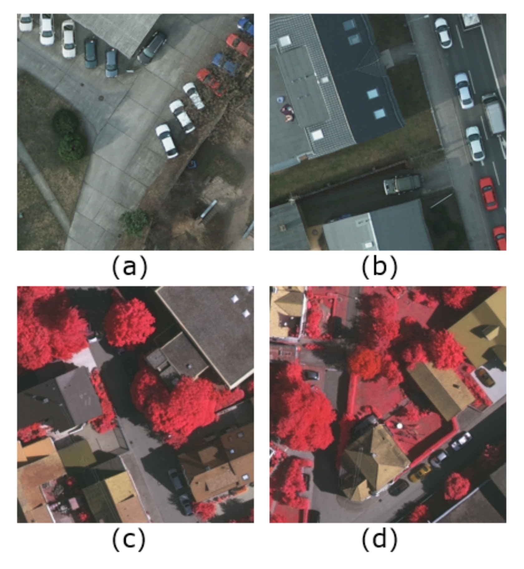
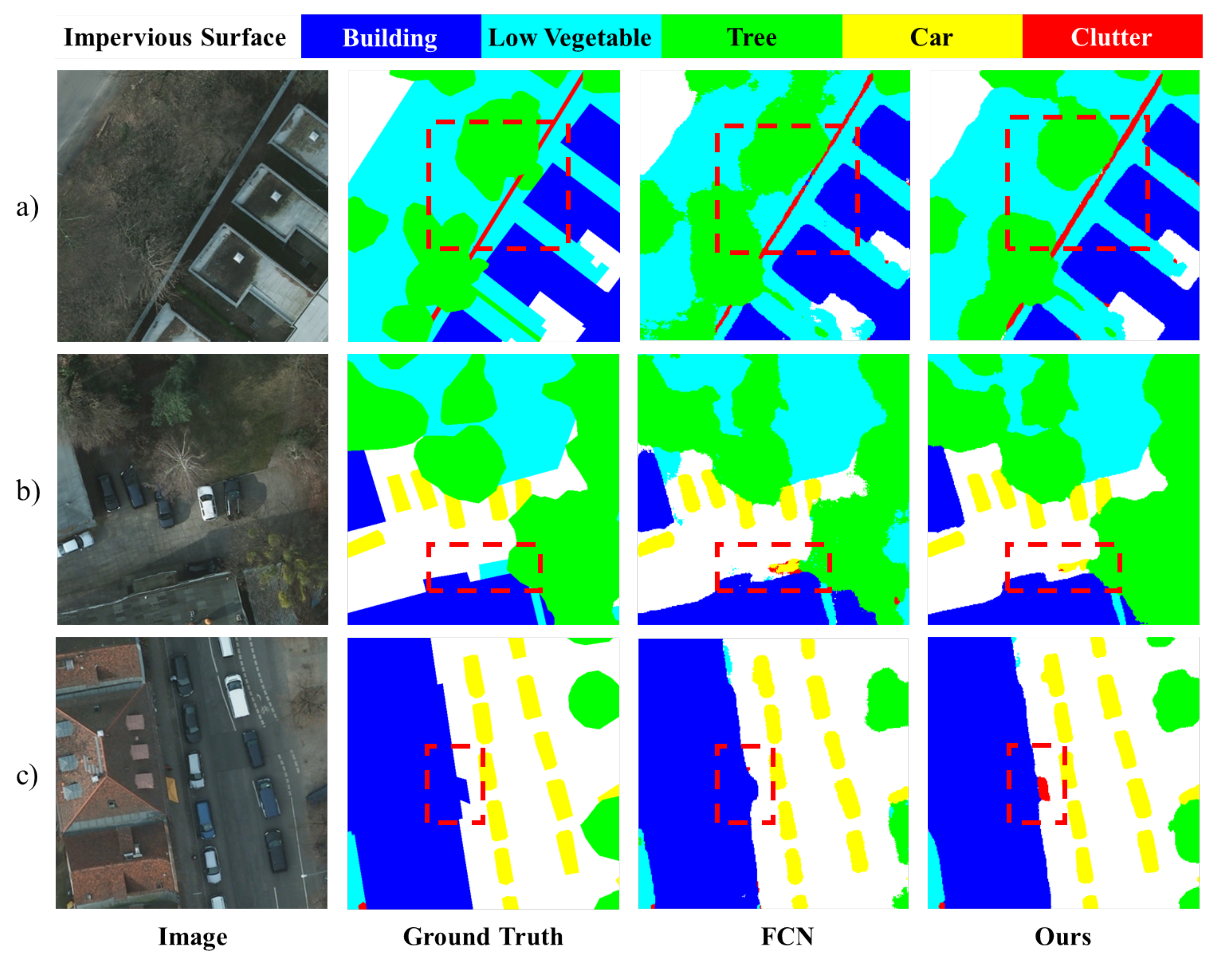
• In the case of images with high resolution, the scale of the foreground object varies greatly (the car in Figure 1a and the building in (b) are both foreground objects, but the scale difference is great).
• The edge of some foreground object is irregular (the tree edge is irregular in Figure 1c,d).
• The background is highly complex and contains a wide variety of features.

Existing semantic segmentation methods are difficult to deal with the complex context information of aerial images. To address the above challenges, a semantic segmentation method is proposed for aerial images based on superpixel-GNN with attention mechanism. First, the aerial image is segmented into superpixels. A graph consisting of all these superpixels as its nodes is then built. Finally, edges are constructed by finding neighbors in the spatial connection between these nodes (superpixels). For each node, the image feature vector (i.e., the output of semantic segmentation CNN) is taken as the initial representation and updated iteratively using recursive functions. The key idea of this dynamic programming approach is that the state of each node is determined by its historical state and the information sent from its neighbors. The aggregation of neighbor information can be differentiated by adding the attention mechanism into the aggregation process. The final state of each node is used to classify each node. Back-Propagation Through Time (BPTT) algorithm is used to calculate the gradient of GNN. In summary, the main contributions of this paper are outlined as follows.

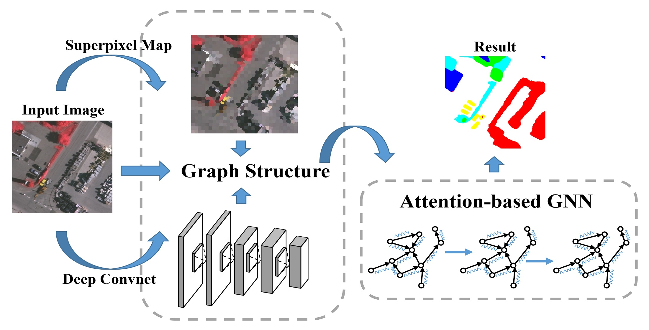
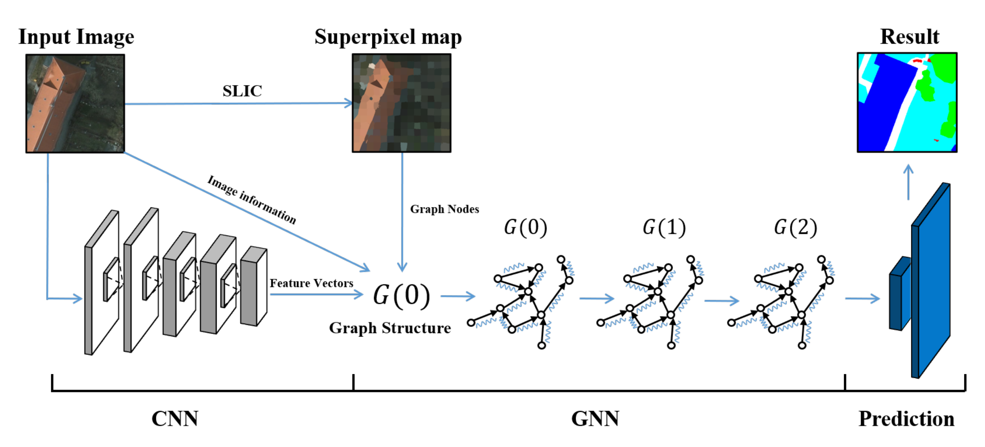
• A GNN-based framework has been proposed for semantic segmentation of aerial images. To get a satisfactory segmentation boundary, superpixels are used as graph nodes for classification, and GNN can learn its representation directly from superpixel graphs. To solve the problem of irregular object edges in aerial images, superpixels are used as graph nodes to construct the graph structure, and GNN can directly learn its representation from the superpixel graph. To overcome the limitations of GNN in extracting features, CNN is used as a feature extractor to provide good feature vectors for the subsequent learning of GNN. Our method takes the complementary advantages of two neural networks (image features extracted by CNN and spatial relations provided by GNN) based on superpixels to achieve satisfactory segmentation results.
• The GNN model in our framework of semantic segmentation of aerial images is an improved version that has introduced the attention mechanism into each node. When the information of neighbor nodes is fused, nodes are aggregated differently depending on their similarity to neighbors, so that the GNN’s expression ability is enhanced. For the challenge of large variation in aerial image scales, we increase the receptive field by increasing the number of neighbors of the graph node when constructing the graph and adding an attention mechanism when merging neighbors’ information. These designs can effectively reduce information fluctuations caused by scale changes, and thus deal with the problem of scale changes. Experimental results show that it has advanced performance on the challenging public datasets of Vaihingen and Potsdam.

The rest of this article is organized as follows. Section 2 covers the latest progress in semantic segmentation of aerial images in two aspects: semantic segmentation and graph neural network. Section 3 describes our proposed SAGNN architecture in detail. Section 4 presents the experiment and result analysis. Finally, the conclusion and future work prospects are given in Section 5.

2. Related Work

2.1. Semantic Segmentation

In recent years, deep learning has become a mainstream method for semantic segmentation. Long et al. first proposed a Full Convolutional Network (FCN) incorporating the upsample convolution layer into Convolutional Neural Network (CNN) to achieve image segmentation of arbitrary size [9]. The FCN model has laid a solid foundation for the following semantic segmentation model. The following works [17,18,19,20] aim to implement multiscale feature fusion by expanding the receptive field. For example, DeepLabv1 increases the receptive field through atrous convolution and solves the problem of repeated maximum pooling and subsampling in DCNNs that cause resolution degradation [17]. Next, DeepLabv2 [18] and DeepLabv3 [19] use Atrous Spatial Pyramid Pool (ASPP), which is composed of parallel convolutions with distinct expansion rates, to capture the image’s context information in multiple proportions. Pyramid Scene Parsing Network (PSPNet) [20] proposed a Pyramid Pooling Module (PPM) to aggregate the contextual information from different regions, thereby improving the ability to obtain global information. Other works [21,22] use an encoder–decoder architecture to optimize object edge details. Semantic segmentation is also a very challenging task to aerial images. However, in addition to the large-scale changes in most image semantic segmentation datasets [23,24], aerial images also have many challenging problems due to their unique characteristics, such as wide gaps between features within the same class, small foreground object, imbalance between background and foreground, etc. [25]. Michele Volpia and Devis Tuia combined the output and features (bottom-up) and conditions of the multi-task CNN coded with the empty field model (top-bottom) to optimize the label space [26]. In addition to increasing the diversity of data, the work in [27] also introduces a Channel Attention Mechanism (CAM), which allows the model to better weigh semantic information and spatial location information, and to achieve more accurate segmentation. Hybrid Multiple Attention Network (HMANet), in order to comprehensively capture the feature correlation among space, channel, and category, three attention modules have been proposed, namely, Class Augmented Attention (CAA), Class Channel Attention (CCA), and Region Shuffle Attention (RSA) [28]. The latest research has proposed the PointFlow Module (PFM). In order to bridge the semantic gap and address the imbalance between foreground and background at the same time, Li et al. designed the PointFlow Network (PFNet) by adding PointFlow Module(PFM) to Feature Pyramid Networks (FPNs) [29].

2.2. Graph Neural Network

There are two main research directions of graph neural networks: One direction is to extend the convolution operation from traditional data (such as images) to graphic data. Graph Convolutional Neural Network (GCNN)-based algorithms are mainly divided into two categories: spectral-based and spatial-based. The spectral-based method defines graph convolution as a filter, so the graph convolution operation is considered to remove noise from the graph signal [30]. On the other hand, the spatial-based method interprets graph convolution as an aggregation of feature information from the neighborhood and coarsens the graph into a high-level substructure through the interleaving arrangement of the graph convolution layer and the graph pooling layer [31]. The other direction is to apply the Recurrent Neural Network (RNN) to each node of the graph [32,33,34,35], thus generating the “graph neural network”. This GNN is based on recursive operators and can be extended to various graph types [32]. Some subsequent works integrated the attention mechanism [13,36,37], autoencoder [14,38], generative network [39,40], and other structures into the GNNs. With the vigorous development of GNN models, their applications have become more and more extensive in various fields, such as social networks [41], recommendation systems [42], life sciences [43], and so on. For unstructured data such as images, superpixels can transform images into graph structures, thus solving image-related tasks using graph neural networks [44,45,46]. Note that the application of GNNs in the field of computer vision, where semantic segmentation is an important task, has attracted more and more attention. Surprisingly, the GNN exhibits extraordinary performance in semantic segmentation tasks. In the semantic segmentation of 3D point cloud images, the work [47] proposes an end-to-end 3DGNN, from which a K-nearest neighbor graph is constructed in 2D pixels according to the depth image, so that the purpose of learning its representation directly from the 3D point cloud can be achieved. The work in [48] proposed the EdgeConv layer to improve the segmentation accuracy by acquiring local features. The result of KNN will differ, depending on the K nearest points re-found, each time the EdgeConv feature is updated according to the distance to the new feature, and the local map constructed each time will be subject to dynamic update. Different from the structure of the KNN structure map, the work [49] proposed the similar concept of superpoint to superpixel to represent simple objects. The superpoint map connected by superpoints performs well in large-scale point cloud semantic segmentation. Similarly, the work [15] of semantic analysis of two-dimensional images also constructs graph structures through superpixels and uses the novel graph Long Short-Term Memory (LSTM) to capture the semantic relationship between superpixels based on local context interactions. The subsequent work [16] proposed a structurally evolved LSTM, which randomly merges graph nodes with high similarity through stacked LSTM layers.

3. Methodology

In this section, the proposed superpixel-based graph semantic segmentation model is presented in details. An overview of the proposed model is introduced followed the description of the superpixel-based graph construction method. Finally, the superpixel-based GNN with attention mechanism is presented.

3.1. Overview of the Graph Structure

The graph structure is shown in Figure 2. The input RGB image is first subjected to superpixel segmentation processing, which can be done off-line. Meanwhile, a stack of convolution layers is used to determine the feature vectors for each RGB image, which are the initial hidden representations of the graph nodes. The graph is built on the superpixel nodes and their spatial connections. More details can be found in Section 3.2. As a result, both semantic information and geometrical information are accessible in this GNN, which consists of three layers. Then a Multi-Layer Perceptron (MLP) with a softmax layer is shared by all graph nodes.

3.2. Graph Construction

Based on the Simple Linear Iterative Clustering (SLIC) superpixel method put forward by Achanta et al. [50], the superpixel-based graph semantic segmentation model is proposed hereof. First, the SLIC approach is used to a generate a superpixel graph. We construct a directed graph based on the superpixel nodes. Each superpixel is regarded as a graph node and each graph node is connected to its K nearest neighbors via directed edges. The graph can be denoted by $G=(V,E,H)$ where V, E, and H represent the sets of nodes, edges, and hidden states, respectively. It can be easily found that the graph is directed and asymmetric. Second, a CNN is used to figure out the feature map which can exploit semantic information. Finally, the feature vectors of the superpixels are determined according to the feature maps and put into the corresponding hidden states of graph nodes.

3.2.1. Nodes Determination

The SLIC method is employed to derive the superpixel graph, in which each superpixel is regarded as a graph node. It is a local clustering method of pixels defined in the 5D space including the $(l,a,b)$ values of the CIELab (Commission International Eclairage Lab) color space and the $(u,v)$ pixel coordinates. In this method, the number of superpixels (nodes) can be specified according to the task and computing power. For smaller granularity segmentation and higher computing power, more superpixels (nodes) can be designed, and vice versa.

3.2.2. Node Features and Labels

Each graph node includes RGB, superpixel center coordinate, and feature information, respectively. As a result, a graph node feature contains following elements: R, G, B, x, y, $label$, and S. Among them, R, G, and B are the average RGB values of all pixels in each superpixel; (x, y) represents the x- and y-coordinates of the center of the superpixel; and S is the feature vector extracted from the convolution feature maps. In subsequent experiments, the improved VGG-16 network, namely, Deeplab-Largefov [17], is used as our unary CNN to extract appearance features from aerial images. The fc7 feature maps are used to upsample the size of the original image, and the size of the output feature maps is H × W × C, where H, W, and C are original height, width, and channel size (1024), respectively. Therefore, the dimension of S is 1024.

In this way, the feature or initial hidden representation of each node $h_i$ can be written as follows:

$$h_i=(R_i,G_i,B_i,x_i,y_i,label,S_i)$$

(1)

$label$ of graph node is the same as the label of corresponding superpixel node. The label of a superpixel node is obtained by voting by the pixels it contains, and the label with the most votes represents the label of this superpixel node.

3.2.3. Edges Determination

Each graph node is connected to its K nearest neighbors which are found in terms of Euclidean distance. When constructing the edge, we add the direction (from the nearest neighbor to the center), and the directional edge can more clearly convey the direction of the information. However, the connection of edges for two graph nodes is not necessarily symmetrical. It means that the edge from node i to node j can not imply the existence of the edge from node j to node i. Algorithm 1 describes the graph construction.

Algorithm 1. Graph Construction.

Input: RGB image

Output: Graph $G=(V,E,H)$

1: compute superpixel map by SLIC method using RGB image

2: each superpixel node is regarded as a graph node

3: graph node → V

4: compute feature map by CNN

5: for each graph node do

6:  compute $R,G,B$

7:  obtain $x,y$ from superpixel center coordinates

8:  compute S

9: $(R,G,B,x,y,S)\to h$, $h\in H$

10: obtain node label in feature map

11: end for

12: for every two nodes i and j do

13: compute Euclidean distance $d_{ij}$ between node i and j

14: end for

15: for every node i do

16: find its K nearest neighbors

17: node i establishes a edge with those K nearest neighbors

18: end for

3.3. Superpixel-Based Attention Graph Neural Network

It can be seen from the above that each graph node has K neighbors, which may have unequal impacts on that node. More attention should be paid to the neighbors which are closer to or have the same label as that node. In other words, these edges should have greater weight [13,37]. As such, we propose the Superpixel-based Attention Graph Neural Network (SAGNN). The overview of SAGNN is shown in Figure 2 and more details can be seen below.

For each node, the propagation process is written as

$$m_i^t=\frac{1}{K}\sum _{j\in N_i}{\mathcal{F}}_1\left({\alpha }_{ij}^t{h}_j^t\right)$$

(2)

$$h_i^{t+1}={\mathcal{F}}_2(h_i^t,m_i^t)$$

(3)

where $N_i$ is the set of K-nearest neighbors of node i;$t\in 0,1,2$ corresponds to graph $G^{\left(0\right)}$, $G^{\left(1\right)}$, and $G^{\left(2\right)}$, respectively; $h_j^t$ is the current hidden state of node j; ${\mathcal{F}}_1$ is a Multi-Layer Perceptron (MLP); $m_i^t$ is a vector, which indicates the aggregation of messages that node i receives from its neighbors $N_i$; ${\alpha }_{ij}^t$ is the attention parameter between node i and node j; and ${\mathcal{F}}_2$ is Vanilla RNN. At each time step, each node collects information from its neighbors by (2), and then fuses its hidden states and neighbors’ information by (3). After that, one can get the next new hidden state $h_i^{t+1}$ of node i which is to be used at the next layer $G^{(t+1)}$. As for attention parameter ${\alpha }_{ij}^t$, it can be obtained by the following equation:

$${\alpha }_{ij}^t=\frac{e^{cos(h_i^t,h_j^t)}}{{\sum }_{j\in N_i}{e}^{cos(h_i^t,h_j^t)}}$$

(4)

${\alpha }_{ij}^t$ is used to represent the correlation between node i and node j, which is measured in terms of the cosine of the angle between their hidden states. ${\alpha }_{ij}^t$ also represents the similarity between two nodes. The higher the similarity between them, the more likely they have the same label. Therefore, higher weight and more attention should be given to the neighbors of nodes with higher similarity.

Finally, the probability over labels can be obtained as follows:

$$p_i={\mathcal{F}}_3\left(h_i^2\right)$$

(5)

where $h_i^2$ is the hidden state of node i in graph $G^{\left(2\right)}$; ${\mathcal{F}}_3$ is a Multi-Layer Perceptron (MLP) with a softmax layer shared by all nodes. Network parameters are adjusted by the Back-Propagation Through Time (BPTT) algorithm.

4. Experimental Results

4.1. Datasets

The proposed method is evaluated using two public benchmarks provided by the International Society for Photogrammetry and Remote Sensing (ISPRS), namely, the Potsdam dataset and the Vaihingen dataset [51]. Both of these datasets consist of the high-resolution True Ortho Photo (TOP), Digital Surface Model (DSM), and ground truth labels.

4.1.1. Potsdam

The Potsdam dataset contains 38 high-resolution images (size 6000 × 6000 pixels), with a Ground Sampling Distance (GSD) of 5 cm. The dataset contains 6 classes: (1) impervious surfaces, (2) building, (3) low vegetation, (4) tree, (5) car, and (6) clutter. The dataset provides four channels of NIR (Near-Infrared)-R-G-B information, DSM, and standardized DSM. Note that DSM is left unused in our experiments. 17 images are used for training and 14 images for testing our model. Each image is cut into 600 × 600 size. The validation set contains 7 images randomly selected from the training set.

4.1.2. Vaihingen

The Vaihingen dataset consists of 33 high-resolution images (average size 2494 × 2064 pixels) with a Ground Sampling Distance (GSD) of 9 cm. The classes of the dataset are the same as those of the Potsdam dataset. The dataset provides NIR-R-G channels and DSM. Sixteen images are used for training and 17 images for testing our model. Each image is cut into 512 × 512 size.

4.2. Evaluation Metrics

On these datasets, our method is evaluated in terms of three commonly used metrics: average F1 score, average accuracy, and Intersection over Union (IoU) [52]. Among them, the F1 score of the foreground object classes is calculated by (6):

$${\mathrm{F}}_1=(1\times {\beta }^2)·\frac{\mathrm{precision}·\mathrm{recall}}{{\beta }^2·+\mathrm{recall}}$$

(6)

where $\beta$ represents the equivalent factor between recall and precision and is usually set to 1. Overall Accuracy (OA) and Intersection over Union (IoU) are defined by Formulas (7) and (8), respectively:

$$\mathrm{OA}=\frac{\mathrm{TN}+\mathrm{TP}}{\mathrm{N}}$$

(7)

$$\mathrm{IoU}=\frac{\mathrm{TP}}{\mathrm{TP}+\mathrm{FN}+\mathrm{FP}}$$

(8)

where: N is the total number of pixels; TN, TP, FN, and FP represent the number of true negatives, true positives, false negatives, and false positives, respectively.

4.3. Implementation Details

In the experiment, the SLIC algorithm [50] is used to generate 2000 superpixels for each image. See Section 4.4 for details about the number of superpixels. Subsequently, the average value of the feature vectors corresponding to all pixels contained in each superpixel is calculated as the average feature vector of the superpixel. Finally, the K nearest neighbors (K = 8 in this experiment) of each superpixel are determined according to the center of the superpixel and the graph structure is constructed. The GNN part is composed of three layers of the same graph structure. The MLP structure of each node is a single layer used to aggregate neighbor information, and the attention parameter $\alpha$ is calculated from forward propagation. In the training phase, the unary CNN is initialized from the pre-trained VGG network in [17]. The network optimization method is Stochastic Gradient Descent (SGD) with momentum, and the norm of the gradient is clipped in order for it not to exceed 10. The initial learning rates of the unary CNN and GNN are 0.001 and 0.01, respectively, the batch size is 5 images, the momentum is 0.9, and the weight attenuation is 0.0001. The MSRA method [53] is used to initialize RNN update functions of our GNN. All the experiments were conducted on the Pytorch framework with NVIDIA GeForce RTX 2080Ti GPU.

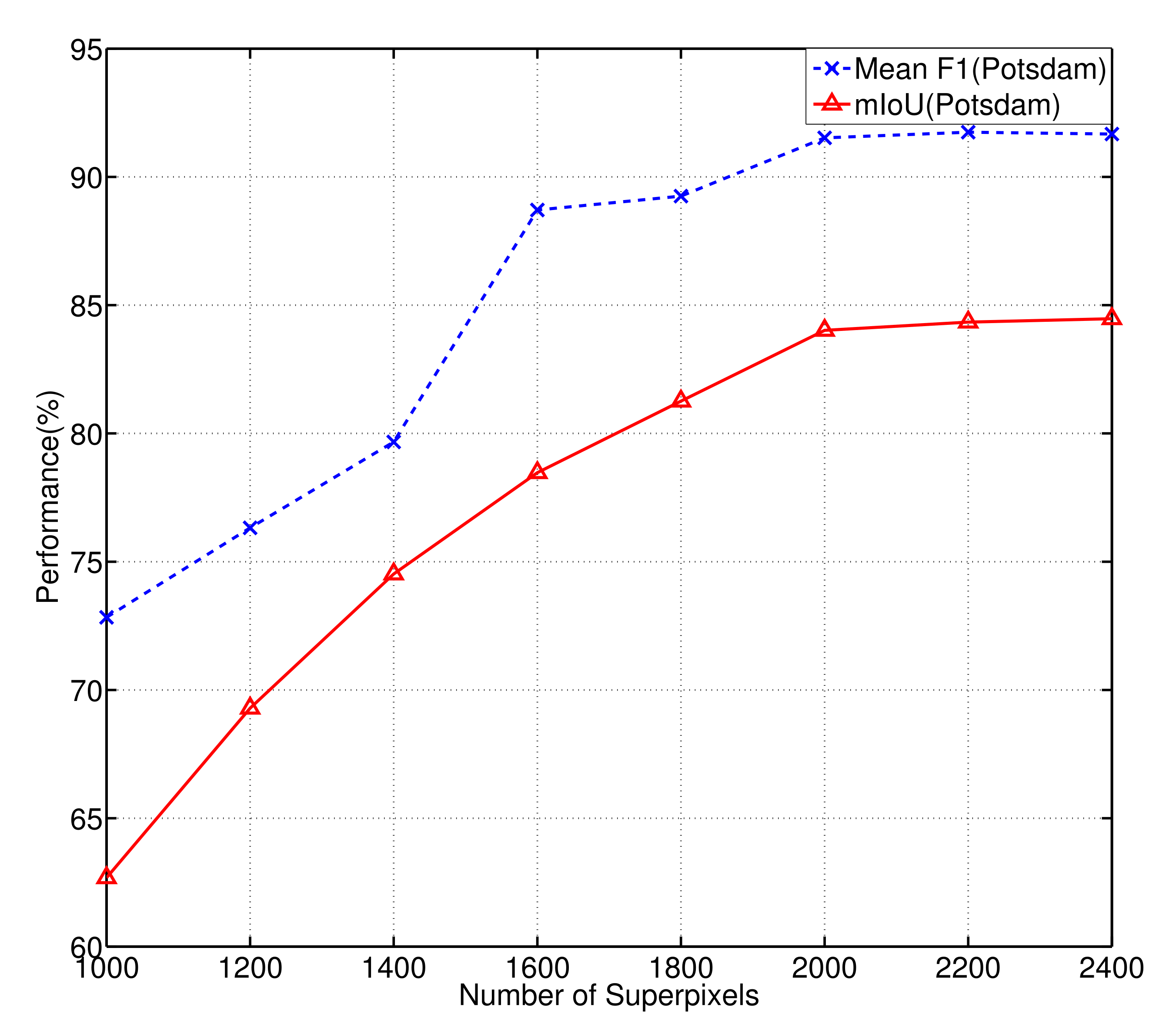
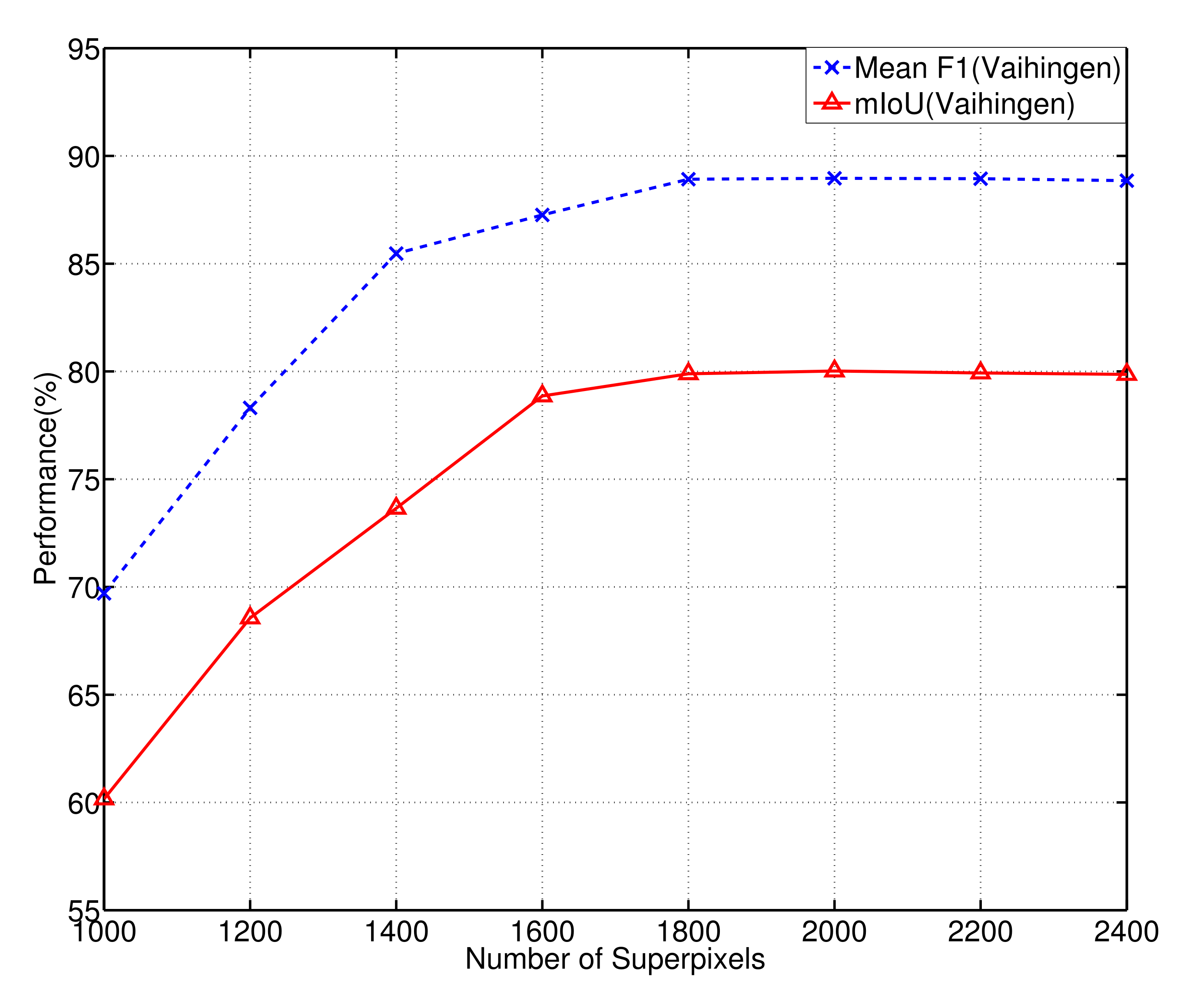
4.4. Superpixel Number

Superpixels can group pixels in advance according to their appearance similarity and spatial correlation, effectively reducing the number of elements for subsequent manipulation and helping preserve the edge information of objects. When the semantic labels of superpixels are defined, most of the internal semantic information of superpixels is consistent and can be directly used as labels. If pixels within a superpixel have different ground truth labels, the voting mechanism is adopted to take the label with the largest proportion as the label of the superpixel. However, superpixels may introduce quantization errors in this case. Therefore, the performance of constructing GNNs is evaluated using different superpixel numbers. Figure 3 and Figure 4 show the experimental results of the Potsdam and Vaihingen datasets at different superpixel numbers, respectively. We can see that, the number of superpixels is preferably greater than 2000 for the Potsdam dataset, and it is better to be greater than 1800 for the Vaihingen dataset. Because the image resolution of the Vaihingen dataset is lower than that of the Potsdam dataset, the Vaihingen dataset needs a lower number of superpixels to achieve maximum accuracy compared to the Potsdam dataset. Comprehensive comparison between the results of the two datasets indicates the network model tends to perform well when more than 2000 superpixels are used. Therefore, in order to balance computational efficiency and prediction accuracy, we used an average of 2000 superpixels for each image throughout the experiment.

4.5. Comparison with Existing Works

Our model was compared with four existing methods, including the benchmark algorithm FCN [9], Spatial propagation CNN (SCNN) [54], RotEqNet [55], and DeepLabV3+ [19]. The experimental results of Potsdam and Vaihingen test sets are shown in

Table 1. Experimental results on Potsdam test set, Bold means best results.

Mehtod	Imp. surf.	Building	Low veg.	Tree	Car	Mean F1	OA (%)	MIoU (%)
FCN [9]	86.81	92.32	82.69	79.25	92.18	86.65	84.67	77.13
SCNN [54]	89.66	92.75	84.23	85.67	93.86	89.23	85.96	81.83
RotEqNet [55]	90.32	93.80	86.94	84.53	94.10	89.94	87.25	82.04
DeeplabV3+ [19]	92.05	94.83	87.79	86.10	95.94	91.34	89.88	83.82
SAGNN (ours)	92.59	95.96	87.86	87.78	96.18	92.01	90.23	84.64

and

Table 2. Experimental results on Vaihingen test set, Bold means best results.

Mehtod	Imp. surf.	Building	Low veg.	Tree	Car	Mean F1	OA (%)	MIoU (%)
FCN [9]	87.26	90.15	75.38	86.14	70.51	81.89	84.57	71.03
SCNN [54]	88.51	91.26	77.65	87.04	79.80	84.85	86.52	74.91
RotEqNet [55]	89.75	93.63	78.60	82.92	77.36	85.25	87.68	76.30
DeeplabV3+ [19]	91.64	94.21	83.11	87.58	86.19	88.55	88.94	79.85
SAGNN (ours)	92.01	95.13	83.09	88.36	87.25	89.16	89.32	80.11

, respectively. In order to directly reflect the segmentation effect, the F1 score is selected as the evaluation metric for each foreground class in Table 1. As shown in Table 1, our SAGNN method not only outperforms other algorithms in F1 scores for each class, but also performs best in mean F1 score, OA and MIoU. Similarly, the numerical results of our method on the Vaihingen test set are also excellent (as shown in Table 2). In addition to the F1 score of Low Vegetables, our SAGNN achieves the best in the other 7 aspects. Our method performs most prominently in Building (in Table 1) and Car (in Table 2), which are 1.13 and 1.06 higher than the sub-optimal algorithm deeplabV3+, respectively. Regardless of whether the segmentation object is large-scale (building) or small-scale (car), our model always achieves good segmentation results, a solid proof that our network is robust to scale changes.

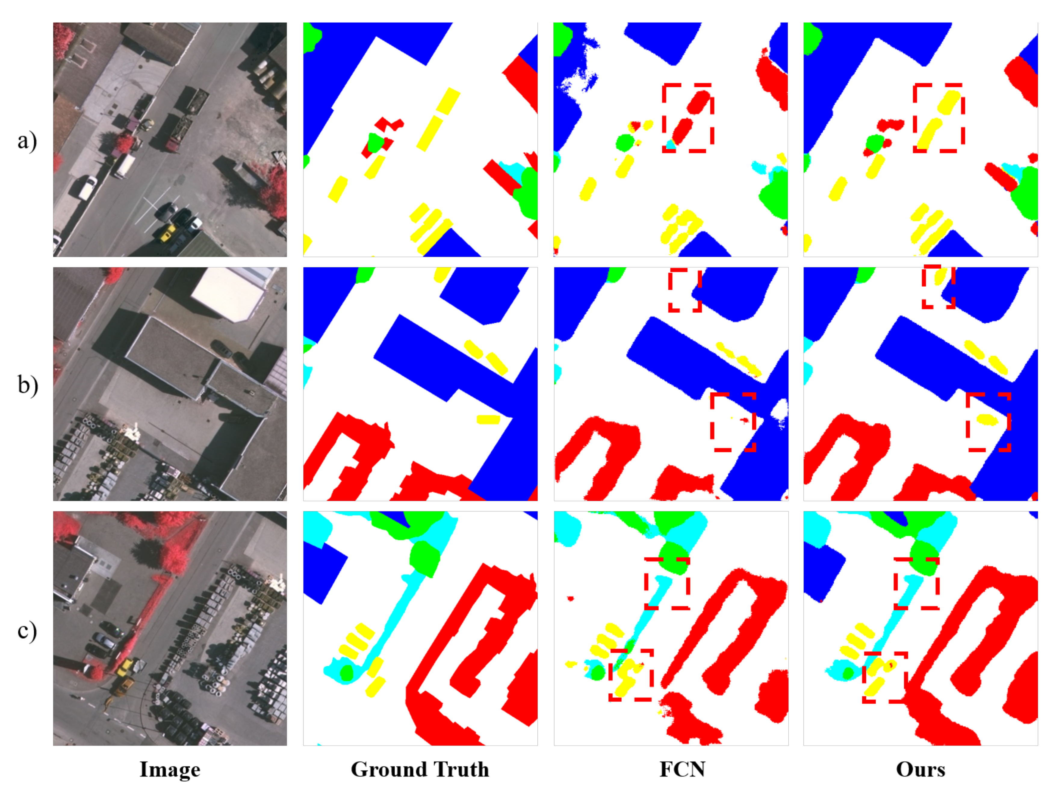
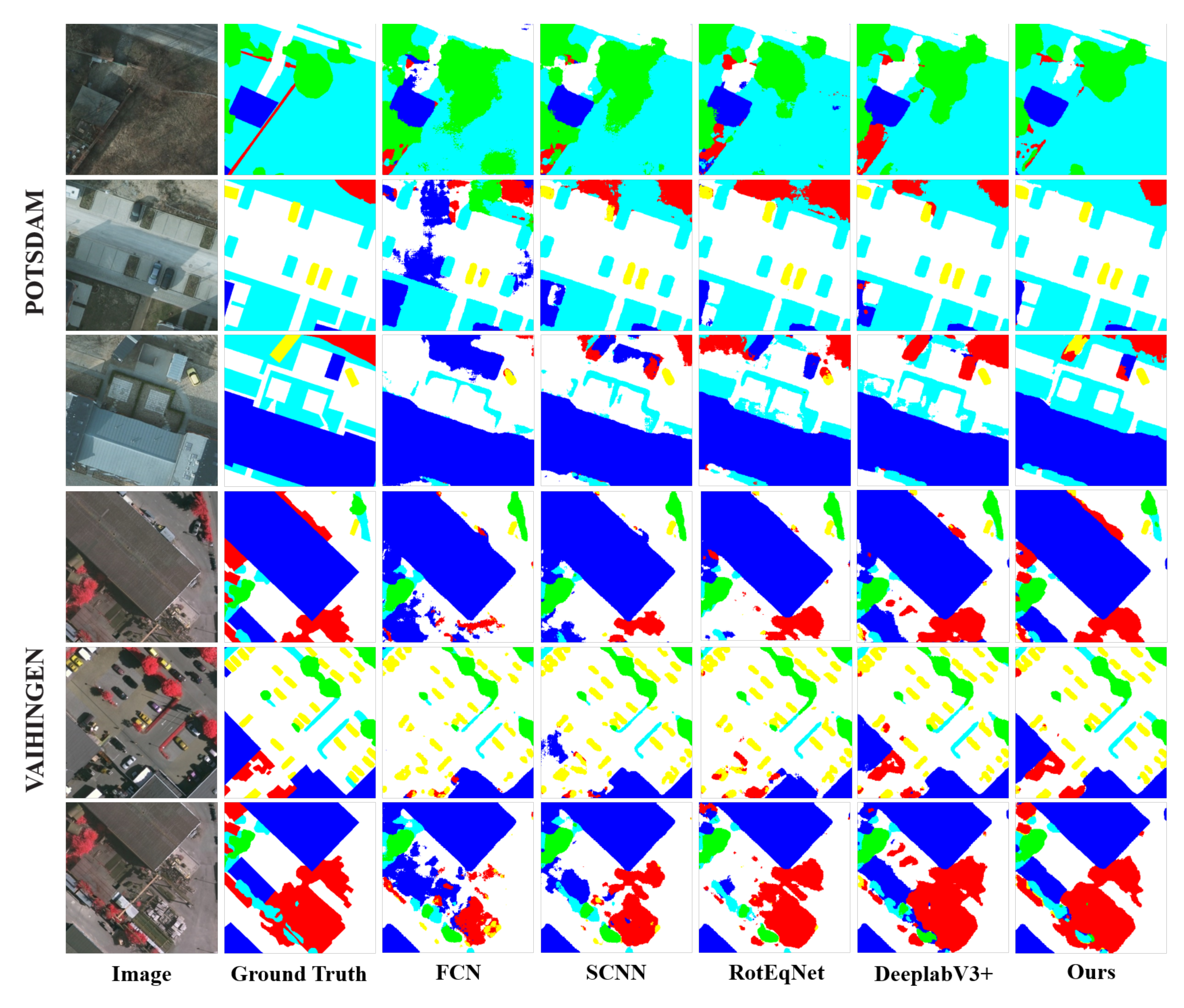
4.6. Qualitative Comparison

The results of qualitative comparison between the Potsdam and Vaihingen test sets for SAGNN and baseline network are provided in Figure 5 and Figure 6, respectively. In particular, the red dotted boxes are used to mark areas that are inaccurately labeled in Figure 5. As the datasets of semantic segmentation are manually annotated, there are label errors, adding more challenges to the inherently difficult semantic segmentation task. From Figure 5, our method is evidently largely superior to the baseline network FCN based algorithm. And the red box in Figure 5a indicates that our model can segment the wall that is not covered by the branches. Similar situations are the black car in Figure 5b, the sunshade in Figure 5c, and the road and the white car in Figure 6c. Even if the Ground Truth is wrong, our model can still give correct predictions. Similarly, SAGNN’s performance is far better than the benchmark on the Vaihingen test set. For example, in the red boxes of Figure 6a,b, the edge is accurately segmented, and the objects are correctly classified, by SAGNN method. In conclusion, SAGNN can predict more accurate segmentation maps; it not only obtains more refined boundary information, but also effectively filters out error noises (incorrectly labeled pixels), a proof of the outstanding performance of GNN and the effectiveness of the model based on superpixels and attention mechanism. Figure 7 shows several examples of the segmentation results of five segmentation algorithms. The upper three rows are the results of the Potsdam test set, and the lower three rows are the results of the Vaihingen test set. The segmentation results of our method are significantly better than those of the other four methods, especially for objects with regular edges (such as Building and Car). However, the segmentation effect is not so accurate for objects with irregular edges, such as the tree in the first image and the low vegetable in the last image.

5. Discussions

5.1. Ablation Study

In SAGNN, three important modules are used on the GNN body: superpixel module, attention module, and (CNN) feature extraction module, among which the superpixel module is used to reduce the resolution of the image and retain the boundary information of the object, the attention module is used to focus on similar neighbor information when clustering neighbors, and the CNN feature extraction module is used to extract feature vectors from the original image. Above is a brief discussion about the contributions of the three modules, with which we conducted ablation studies under different settings.

Table 3. Ablation study on Potsdam test set.

Mehtod	Superpixel	Attention	CNN	OA (%)	MIoU (%)
	✓			84.01	76.95
		✓		82.43	75.16
			✓	84.57	77.02
SAGNN	✓	✓		86.32	81.95
	✓		✓	89.54	83.97
		✓	✓	87.68	82.19
	✓	✓	✓	90.23	84.64

and

Table 4. Ablation study on Vaihingen test set.

Mehtod	Superpixel	Attention	CNN	OA (%)	MIoU (%)
	✓			83.82	70.78
		✓		82.21	70.29
			✓	84.13	71.98
SAGNN	✓	✓		86.45	74.88
	✓		✓	88.17	78.70
		✓	✓	87.39	76.16
	✓	✓	✓	89.32	80.11

show the ablation experiment results on Potsdam and Vaihingen datasets, respectively.

As shown in Table 3, when these three modules are used alone, both overall accuracy and average IoU are below baseline levels. Especially, when the attention module is used alone, the overall model performance is the worst, with OA only 82.72% and MIoU only 75.16%. However, this result does not mean that the attention module is unimportant. The main functions of the attention mechanism are to strengthen effective information and weaken redundant information. For the graph neural network model, the influence of the attention module on the semantic segmentation is indirect, and its greater significance is to increase the ability of the neural network to extract effective information. However, improving the edge accuracy of the image (super-pixel module) and improving feature quality (CNN module) have direct and effective effects on semantic segmentation results, so the model performance will be better when the attention module is used with these two modules. In the experiment where the two modules are used at the same time, it can be seen that the OA of “Superpixel + Attention” combination reaches 86.45%, which is 4.02% higher than if the “Attention” module is used alone, and 2.44% higher than if the “Superpixel” module is used alone; also significant is the improvement brought about with simultaneous use of “Superpixel + Attention” combination in MIoU. Similarly, the OA and MIoU of “Attention + CNN” combination have also achieved better results of 87.68% and 82.19%, respectively. These prove that the attention module has a strong dependence, while the simultaneous use of the other two modules can greatly improve the performance of our model. In the dual-module experiment, the OA and MIoU of “Superpixel + CNN” combination are the best, achieving more than one percentage point higher in each metric than either “Superpixel + Attention” or “Attention + CNN” combination. These results show that good segmentation results require not only superpixel preprocessing but also high-quality features being extracted by CNN. Finally, when the three modules are applied at the same time, OA and mIOU reach the best of all experiments. The same situation can be verified in Table 4. In summary, our method proves effective in optimizing the model from different angles, which brings great benefits to target segmentation.

We also conduct ablation experiments on our method in terms of parameters, inference time on GPU, and computational cost (FLOPs).

Table 5. Ablation study of Parameters (PRM), Inference Time (IT) on GPU, and computational cost (FLOPs).

Mehtod	Superpixel	Attention	CNN	PRM (M)	IT (ms)	FLOPs (Giga)
	✓			7.03	12.96	8.65
		✓		9.20	15.19	16.78
			✓	10.56	16.28	17.80
SAGNN	✓	✓		7.86	14.10	10.24
	✓		✓	8.02	14.24	13.78
		✓	✓	11.21	16.76	18.13
	✓	✓	✓	8.96	15.07	14.51

details the quantitative results of ablation experiments on the Potsdam test set. It can be seen from Table 5 that the addition of the superpixel module can save inference time and computational cost very effectively.

5.2. Extensive Analysis

We list five aerial images semantic segmentation datasets in

Table 6. Comparison of 5 aerial image semantic segmentation datasets.

Method	Dataset	Original Size	No.	Class	Patch Size
Multi-task learning [26]	Zeebrugges	10K × 10K	7	8	500 × 500
DMSMR [56]	EvLab-SS	4500 × 4500	60	11	321 × 321
CNN–MRS [57]	Zurich Summer	1100 × 1100	20	8	128 × 128
SAGNN	Potsdam	6000 × 6000	38	6	600 × 600
SAGNN	Vaihingen	2494 × 2064	33	6	512 × 512

. Among them, the single sheet with the highest resolution is the Zeebrugges dataset, with a spatial resolution of 5 cm. In order to improve computational efficiency, the method [26] reduced the spatial resolution to 10 cm. The largest number of images is The EvLab-SS dataset, which contains 35 satellite images and 25 aerial images. Dual Multi-Scale Manifold Ranking (DMSMR) Network [56] cut the images into 640 × 480 pixels patches and then compresses them into 321 × 321 pixels for training. The Zurich Summer dataset is a relatively small dataset compared to the other four datasets. CNN-Multiresolution Segmentation (MRS) [57] designed three patch sizes (32 × 32, 64 × 64, 128 × 128) for training. P dataset and V dataset are commonly used aerial image semantic segmentation datasets. In order to ensure that the image information is relatively complete, we did not reduce the resolution of the pictures, and cut them into patches of 600 × 600 pixels and 512 × 512 pixels for training. It can be seen from the patch size that our method (including other methods) deals with relatively small-sized patches. For the semantic segmentation model, the learning and processing of large-size images is a challenge, and the substantial increase in image resolution will cause exponential growth in parameters. Our graph structure is constructed with superpixels, so it is advantageous to deal with large-size images. As the image size reaches the city-scale, our model can upgrade the graph neural network to a dynamic evolution network to save computing resources and merge graph nodes in the learning process.

6. Conclusions

In this work, a superpixel-based attention graph neural network was proposed for semantic segmentation of aerial images. GNN was built on superpixel nodes and features extracted from the image, with an attention mechanism introduced into the propagation process. Our SAGNN used both the appearance information of aerial images and the geometrical relationship between superpixels. It was able to capture long-term dependencies in images more effectively and maintain the integrity of semantic information. The comprehensive evaluation of two public datasets for semantic segmentation of aerial images well demonstrated that our SAGNN had superior performance. The evaluation metrics on both datasets attained the best results. Although the edges of objects of aerial images are irregular, our model was able segment them accurately. Our model achieved the highest F1 scores regardless of object scale, which showed that our model was robust to aerial images with large scale changes. Although our model performed well in the semantic segmentation task of aerial images, there are still unresolved problems, such as how to process larger size aerial images. As such, a direction of our future work will be to explore how to achieve semantic segmentation of large-size aerial images using a dynamic evolution graph neural network.

References

1. Maggiori, E.; Tarabalka, Y.; Charpiat, G.; Alliez, P. High-resolution aerial image labeling with convolutional neural networks. IEEE Trans. Geosci. Remote Sens. 2017, 55, 7092–7103. [Google Scholar] [CrossRef] [Green Version]
2. Ratajczak, R.; Crispim-Junior, C.F.; Faure, É.; Fervers, B.; Tougne, L. Automatic land cover reconstruction from historical aerial images: An evaluation of features extraction and classification algorithms. IEEE Trans. Image Process. 2019, 28, 3357–3371. [Google Scholar] [CrossRef] [PubMed]
3. Zhang, Q.; Seto, K.C. Mapping urbanization dynamics at regional and global scales using multi-temporal DMSP/OLS nighttime light data. Remote Sens. Environ. 2011, 115, 2320–2329. [Google Scholar] [CrossRef]
4. Zhang, X.; Ma, W.; Li, C.; Wu, J.; Tang, X.; Jiao, L. Fully convolutional network-based ensemble method for road extraction from aerial images. IEEE Geosci. Remote Sens. Lett. 2019, 17, 1777–1781. [Google Scholar] [CrossRef]
5. Rau, J.Y.; Jhan, J.P.; Hsu, Y.C. Analysis of oblique aerial images for land cover and point cloud classification in an urban environment. IEEE Trans. Geosci. Remote Sens. 2014, 53, 1304–1319. [Google Scholar] [CrossRef]
6. Levner, I.; Zhang, H. Classification-driven watershed segmentation. IEEE Trans. Image Process. 2007, 16, 1437–1445. [Google Scholar] [CrossRef] [PubMed]
7. Gedeon, T.; Parker, A.E.; Campion, C.; Aldworth, Z. Annealing and the normalized N-cut. Pattern Recognit. 2008, 41, 592–606. [Google Scholar] [CrossRef] [Green Version]
8. Rother, C.; Kolmogorov, V.; Blake, A. “GrabCut” interactive foreground extraction using iterated graph cuts. ACM Trans. Graph. (TOG) 2004, 23, 309–314. [Google Scholar] [CrossRef]
9. Long, J.; Shelhamer, E.; Darrell, T. Fully convolutional networks for semantic segmentation. In Proceedings of the IEEE Conference on Computer Vision and Pattern Recognition, Boston, MA, USA, 7–12 June 2015; pp. 3431–3440. [Google Scholar]
10. Xiao, T.; Liu, Y.; Zhou, B.; Jiang, Y.; Sun, J. Unified perceptual parsing for scene understanding. In Proceedings of the European Conference on Computer Vision (ECCV), Munich, Germany, 8–14 September 2018; pp. 418–434. [Google Scholar]
11. Zhang, Z.; Zhang, X.; Peng, C.; Xue, X.; Sun, J. Exfuse: Enhancing feature fusion for semantic segmentation. In Proceedings of the European Conference on Computer Vision (ECCV), Munich, Germany, 8–14 September 2018; pp. 269–284. [Google Scholar]
12. Huang, Z.; Wang, X.; Huang, L.; Huang, C.; Wei, Y.; Liu, W. Ccnet: Criss-cross attention for semantic segmentation. In Proceedings of the IEEE/CVF International Conference on Computer Vision, Seoul, Korea, 27–28 October 2019; pp. 603–612. [Google Scholar]
13. Veličković, P.; Cucurull, G.; Casanova, A.; Romero, A.; Lio, P.; Bengio, Y. Graph attention networks. arXiv 2017, arXiv:1710.10903. [Google Scholar]
14. Yu, W.; Zheng, C.; Cheng, W.; Aggarwal, C.C.; Song, D.; Zong, B.; Chen, H.; Wang, W. Learning deep network representations with adversarially regularized autoencoders. In Proceedings of the 24th ACM SIGKDD International Conference on Knowledge Discovery & Data Mining, London, UK, 19–23 August 2018; pp. 2663–2671. [Google Scholar]
15. Liang, X.; Shen, X.; Feng, J.; Lin, L.; Yan, S. Semantic object parsing with graph lstm. In Proceedings of the European Conference on Computer Vision, Amsterdam, The Netherlands, 11–14 October 2016; Springer: Berlin/Heidelberg, Germany, 2016; pp. 125–143. [Google Scholar]
16. Liang, X.; Lin, L.; Shen, X.; Feng, J.; Yan, S.; Xing, E.P. Interpretable structure-evolving lstm. In Proceedings of the IEEE Conference on Computer Vision and Pattern Recognition, Honolulu, HI, USA, 21–26 July 2017; pp. 1010–1019. [Google Scholar]
17. Chen, L.C.; Papandreou, G.; Kokkinos, I.; Murphy, K.; Yuille, A.L. Semantic image segmentation with deep convolutional nets and fully connected crfs. arXiv 2014, arXiv:1412.7062. [Google Scholar]
18. Chen, L.C.; Papandreou, G.; Kokkinos, I.; Murphy, K.; Yuille, A.L. Deeplab: Semantic image segmentation with deep convolutional nets, atrous convolution, and fully connected crfs. IEEE Trans. Pattern Anal. Mach. Intell. 2017, 40, 834–848. [Google Scholar] [CrossRef]
19. Chen, L.C.; Papandreou, G.; Schroff, F.; Adam, H. Rethinking atrous convolution for semantic image segmentation. arXiv 2017, arXiv:1706.05587. [Google Scholar]
20. Zhao, H.; Shi, J.; Qi, X.; Wang, X.; Jia, J. Pyramid scene parsing network. In Proceedings of the IEEE Conference on Computer Vision and Pattern Recognition, Honolulu, HI, USA, 21–26 July 2017; pp. 2881–2890. [Google Scholar]
21. Ronneberger, O.; Fischer, P.; Brox, T. U-net: Convolutional networks for biomedical image segmentation. In Proceedings of the International Conference on Medical Image Computing and Computer-Assisted Intervention, Munich, Germany, 5–9 October 2015; Springer: Berlin/Heidelberg, Germany, 2015; pp. 234–241. [Google Scholar]
22. Badrinarayanan, V.; Kendall, A.; Cipolla, R. Segnet: A deep convolutional encoder-decoder architecture for image segmentation. IEEE Trans. Pattern Anal. Mach. Intell. 2017, 39, 2481–2495. [Google Scholar] [CrossRef]
23. Caesar, H.; Uijlings, J.; Ferrari, V. Coco-stuff: Thing and stuff classes in context. In Proceedings of the IEEE Conference on Computer Vision and Pattern Recognition, Salt Lake City, UT, USA, 18–22 June 2018; pp. 1209–1218. [Google Scholar]
24. Cordts, M.; Omran, M.; Ramos, S.; Rehfeld, T.; Enzweiler, M.; Benenson, R.; Franke, U.; Roth, S.; Schiele, B. The cityscapes dataset for semantic urban scene understanding. In Proceedings of the IEEE Conference on Computer Vision and Pattern Recognition, Las Vegas, NV, USA, 27–30 June 2016; pp. 3213–3223. [Google Scholar]
25. Waqas Zamir, S.; Arora, A.; Gupta, A.; Khan, S.; Sun, G.; Shahbaz Khan, F.; Zhu, F.; Shao, L.; Xia, G.S.; Bai, X. isaid: A large-scale dataset for instance segmentation in aerial images. In Proceedings of the IEEE/CVF Conference on Computer Vision and Pattern Recognition Workshops, Long Beach, CA, USA, 16–17 June 2019; pp. 28–37. [Google Scholar]
26. Volpi, M.; Tuia, D. Deep multi-task learning for a geographically-regularized semantic segmentation of aerial images. ISPRS J. Photogramm. Remote Sens. 2018, 144, 48–60. [Google Scholar] [CrossRef] [Green Version]
27. Luo, H.; Chen, C.; Fang, L.; Zhu, X.; Lu, L. High-Resolution Aerial Images Semantic Segmentation Using Deep Fully Convolutional Network With Channel Attention Mechanism. IEEE J. Sel. Top. Appl. Earth Obs. Remote Sens. 2019, 12, 3492–3507. [Google Scholar] [CrossRef]
28. Niu, R.; Sun, X.; Tian, Y.; Diao, W.; Chen, K.; Fu, K. Hybrid multiple attention network for semantic segmentation in aerial images. IEEE Trans. Geosci. Remote Sens. 2021, 60, 5603018. [Google Scholar] [CrossRef]
29. Li, X.; He, H.; Li, X.; Li, D.; Cheng, G.; Shi, J.; Weng, L.; Tong, Y.; Lin, Z. PointFlow: Flowing semantics through points for aerial image segmentation. In Proceedings of the IEEE/CVF Conference on Computer Vision and Pattern Recognition, Nashville, TN, USA, 19–25 June 2021; pp. 4217–4226. [Google Scholar]
30. Defferrard, M.; Bresson, X.; Vandergheynst, P. Convolutional neural networks on graphs with fast localized spectral filtering. Adv. Neural Inf. Process. Syst. 2016, 29, 3844–3852. [Google Scholar]
31. Dai, H.; Kozareva, Z.; Dai, B.; Smola, A.; Song, L. Learning steady-states of iterative algorithms over graphs. In Proceedings of the International Conference on Machine Learning, PMLR, Stockholm, Sweden, 10–15 July 2018; pp. 1106–1114. [Google Scholar]
32. Gori, M.; Monfardini, G.; Scarselli, F. A new model for learning in graph domains. In Proceedings of the 2005 IEEE International Joint Conference on Neural Networks, Montreal, QC, Canada, 31 July–4 August 2005; Volume 2, pp. 729–734. [Google Scholar]
33. Li, Y.; Tarlow, D.; Brockschmidt, M.; Zemel, R. Gated graph sequence neural networks. arXiv 2015, arXiv:1511.05493. [Google Scholar]
34. Scarselli, F.; Gori, M.; Tsoi, A.C.; Hagenbuchner, M.; Monfardini, G. The graph neural network model. IEEE Trans. Neural Netw. 2008, 20, 61–80. [Google Scholar] [CrossRef] [Green Version]
35. Tai, K.S.; Socher, R.; Manning, C.D. Improved semantic representations from tree-structured long short-term memory networks. arXiv 2015, arXiv:1503.00075. [Google Scholar]
36. Lee, J.B.; Rossi, R.; Kong, X. Graph classification using structural attention. In Proceedings of the 24th ACM SIGKDD International Conference on Knowledge Discovery & Data Mining, London, UK, 19–23 August 2018; pp. 1666–1674. [Google Scholar]
37. Thekumparampil, K.K.; Wang, C.; Oh, S.; Li, L.J. Attention-based graph neural network for semi-supervised learning. arXiv 2018, arXiv:1803.03735. [Google Scholar]
38. Tu, K.; Cui, P.; Wang, X.; Yu, P.S.; Zhu, W. Deep recursive network embedding with regular equivalence. In Proceedings of the 24th ACM SIGKDD International Conference on Knowledge Discovery & Data Mining, London, UK, 19–23 August 2018; pp. 2357–2366. [Google Scholar]
39. Bojchevski, A.; Shchur, O.; Zügner, D.; Günnemann, S. Netgan: Generating graphs via random walks. In Proceedings of the International Conference on Machine Learning, PMLR, Stockholm, Sweden, 10–15 July 2018; pp. 610–619. [Google Scholar]
40. You, J.; Ying, R.; Ren, X.; Hamilton, W.; Leskovec, J. Graphrnn: Generating realistic graphs with deep auto-regressive models. In Proceedings of the International Conference on Machine Learning, PMLR, Stockholm, Sweden, 10–15 July 2018; pp. 5708–5717. [Google Scholar]
41. Min, S.; Gao, Z.; Peng, J.; Wang, L.; Qin, K.; Fang, B. STGSN—A Spatial–Temporal Graph Neural Network framework for time-evolving social networks. Knowl. Based Syst. 2021, 214, 106746. [Google Scholar] [CrossRef]
42. Tao, Y.; Wang, C.; Yao, L.; Li, W.; Yu, Y. Item trend learning for sequential recommendation system using gated graph neural network. Neural Comput. Appl. 2021, 1–16. [Google Scholar] [CrossRef]
43. Zhao, C.; Liu, S.; Huang, F.; Liu, S.; Zhang, W. CSGNN: Contrastive self-supervised graph neural network for molecular interaction prediction. In Proceedings of the Thirtieth International Joint Conference on Artificial Intelligence, Online, 19–27 August 2021; pp. 3756–3763. [Google Scholar]
44. Youn, C.H.; Linh, V.L. Dynamic graph neural network for super-pixel image classification. In Proceedings of the 2021 International Conference on Information and Communication Technology Convergence (ICTC), Jeju Island, Korea, 20–22 October 2021; pp. 1095–1099. [Google Scholar]
45. Avelar, P.H.; Tavares, A.R.; da Silveira, T.L.; Jung, C.R.; Lamb, L.C. Superpixel image classification with graph attention networks. In Proceedings of the 2020 33rd SIBGRAPI Conference on Graphics, Patterns and Images (SIBGRAPI), Porto de Galinhas, Brazil, 7–10 November 2020; pp. 203–209. [Google Scholar]
46. Long, J.; Yan, Z.; Chen, H. A Graph Neural Network for Superpixel Image Classification. J. Phys. Conf. Ser. 2021, 1871, 012071. [Google Scholar] [CrossRef]
47. Qi, X.; Liao, R.; Jia, J.; Fidler, S.; Urtasun, R. 3d graph neural networks for rgbd semantic segmentation. In Proceedings of the IEEE International Conference on Computer Vision, Venice, Italy, 22–29 October 2017; pp. 5199–5208. [Google Scholar]
48. Wang, Y.; Sun, Y.; Liu, Z.; Sarma, S.E.; Bronstein, M.M.; Solomon, J.M. Dynamic graph cnn for learning on point clouds. ACM Trans. Graph. (TOG) 2019, 38, 1–12. [Google Scholar] [CrossRef] [Green Version]
49. Landrieu, L.; Simonovsky, M. Large-scale point cloud semantic segmentation with superpoint graphs. In Proceedings of the IEEE Conference on Computer Vision and Pattern Recognition, Salt Lake City, UT, USA, 18–23 June 2018; pp. 4558–4567. [Google Scholar]
50. Achanta, R.; Shaji, A.; Smith, K.; Lucchi, A.; Fua, P.; Süsstrunk, S. SLIC superpixels compared to state-of-the-art superpixel methods. IEEE Trans. Pattern Anal. Mach. Intell. 2012, 34, 2274–2282. [Google Scholar] [CrossRef] [Green Version]
51. Rottensteiner, F.; Sohn, G.; Gerke, M.; Wegner, J.D. ISPRS Semantic Labeling Contest; ISPRS: Leopoldshöhe, Germany, 2014. [Google Scholar]
52. Garcia-Garcia, A.; Orts-Escolano, S.; Oprea, S.; Villena-Martinez, V.; Garcia-Rodriguez, J. A review on deep learning techniques applied to semantic segmentation. arXiv 2017, arXiv:1704.06857. [Google Scholar]
53. He, K.; Zhang, X.; Ren, S.; Sun, J. Delving deep into rectifiers: Surpassing human-level performance on imagenet classification. In Proceedings of the IEEE International Conference on Computer Vision, Santiago, Chile, 7–13 December 2015; pp. 1026–1034. [Google Scholar]
54. Pan, X.; Shi, J.; Luo, P.; Wang, X.; Tang, X. Spatial as deep: Spatial cnn for traffic scene understanding. In Proceedings of the Thirty-Second AAAI Conference on Artificial Intelligence, New Orleans, LA, USA, 2–7 February 2018. [Google Scholar]
55. Marcos, D.; Volpi, M.; Kellenberger, B.; Tuia, D. Land cover mapping at very high resolution with rotation equivariant CNNs: Towards small yet accurate models. ISPRS J. Photogramm. Remote Sens. 2018, 145, 96–107. [Google Scholar] [CrossRef] [Green Version]
56. Zhang, M.; Hu, X.; Zhao, L.; Lv, Y.; Luo, M.; Pang, S. Learning dual multi-scale manifold ranking for semantic segmentation of high-resolution images. Remote Sens. 2017, 9, 500. [Google Scholar] [CrossRef] [Green Version]
57. Atik, S.O.; Ipbuker, C. Integrating Convolutional Neural Network and Multiresolution Segmentation for Land Cover and Land Use Mapping Using Satellite Imagery. Appl. Sci. 2021, 11, 5551. [Google Scholar] [CrossRef]
Figure 1. Illustration of image from two public aerial image semantic segmentation datasets: (a,b) are from the Potsdam dataset and (c,d) are from the Vaihingen dataset.
Remotesensing 14 00305 g001
Figure 2. The left half of Figure 2 is an illustration of the diagram construction. The superpixels obtained by SLIC segmentation of aerial images are used as graph nodes, feature vectors extracted by convolutional neural networks and picture information (RGB, label, and coordinate information) are used as the hidden state of nodes, and k-nearest neighbors graph is constructed according to the spatial relations between superpixels. The blue curve in the graph neural network represents the addition of attention in information aggregation, which can aggregate neighbor information differently. Finally, we get the segmentation result of aerial image through prediction module.
Remotesensing 14 00305 g002
Figure 3. Performance comparisons of different superpixel numbers when evaluating on Potsdam dataset.
Remotesensing 14 00305 g003
Figure 4. Performance comparisons of different superpixel numbers when evaluating on Vaihingen dataset.
Remotesensing 14 00305 g004
Figure 5. Qualitative comparisons between our method and baseline on Potsdam test set.
Remotesensing 14 00305 g005
Figure 6. Qualitative comparisons between our method and baseline on Vaihingen test set.
Remotesensing 14 00305 g006
Figure 7. Examples of segmentation results on Potsdam and Vaihingen test sets.
Remotesensing 14 00305 g007