Article

Performance and Sensitivity of Individual Tree Segmentation Methods for UAV-LiDAR in Multiple Forest Types

1
Research Center of Forestry Remote Sensing & Information Engineering, Central South University of Forestry and Technology, Changsha 410004, China
2
Key Laboratory of Forestry Remote Sensing Based Big Data & Ecological Security for Hunan Province, Changsha 410004, China
3
Key Laboratory of State Forestry Administration on Forest Resources Management and Monitoring in Southern Area, Changsha 410004, China
4
Department of Forest Inventory and Monitoring, Central South Inventory and Planning Institute of National Forestry and Grassland Administration, Changsha 410004, China
5
Research Institute of Forest Resource Information Techniques, Chinese Academy of Forestry, Beijing 100091, China
6
Shanghai Huace Navigation Technology Ltd., Shanghai 201702, China
*
Author to whom correspondence should be addressed.
Remote Sens. 2022, 14(2), 298; https://doi.org/10.3390/rs14020298
Submission received: 25 November 2021 / Revised: 6 January 2022 / Accepted: 7 January 2022 / Published: 10 January 2022
(This article belongs to the Collection Feature Paper Special Issue on Forest Remote Sensing)

Abstract

:
Using unmanned aerial vehicles (UAV) as platforms for light detection and ranging (LiDAR) sensors offers the efficient operation and advantages of active remote sensing; hence, UAV-LiDAR plays an important role in forest resource investigations. However, high-precision individual tree segmentation, in which the most appropriate individual tree segmentation method and the optimal algorithm parameter settings must be determined, remains highly challenging when applied to multiple forest types. This article compared the applicability of methods based on a canopy height model (CHM) and a normalized point cloud (NPC) obtained from UAV-LiDAR point cloud data. The watershed algorithm, local maximum method, point cloud-based cluster segmentation, and layer stacking were used to segment individual trees and extract the tree height parameters from nine plots of three forest types. The individual tree segmentation results were evaluated based on experimental field data, and the sensitivity of the parameter settings in the segmentation methods was analyzed. Among all plots, the overall accuracy F of individual tree segmentation was between 0.621 and 1, the average RMSE of tree height extraction was 1.175 m, and the RMSE% was 12.54%. The results indicated that compared with the CHM-based methods, the NPC-based methods exhibited better performance in individual tree segmentation; additionally, the type and complexity of a forest influence the accuracy of individual tree segmentation, and point cloud-based cluster segmentation is the preferred scheme for individual tree segmentation, while layer stacking should be used as a supplement in multilayer forests and extremely complex heterogeneous forests. This research provides important guidance for the use of UAV-LiDAR to accurately obtain forest structure parameters and perform forest resource investigations. In addition, the methods compared in this paper can be employed to extract vegetation indices, such as the canopy height, leaf area index, and vegetation coverage.

1. Introduction

Forests, representing the main type of terrestrial ecosystem, play an irreplaceable role in maintaining the global climate system, slowing the rise of greenhouse gas concentrations, and achieving carbon neutrality [1,2,3]. Individual trees are the basic units of forests. Hence, accurately obtaining information regarding the attributes of individual trees (tree species, tree height, diameter at breast height (DBH), crown width, etc.) is important for understanding the current state of and changes in forest resources and the ecological benefits of forests, as well as achieving the effective protection and sustainable management of forests [4,5,6].
Traditional forest resource investigation methods explore individual trees in a sample plot with simple and convenient instruments through scientific sampling [7,8]. While this kind of survey method is highly precise and is broadly implemented by forestry departments worldwide, it is also time-consuming, laborious, and destructive to the surveyed vegetation to a certain extent. Moreover, the survey results may not accurately reflect the current state of forest resources across a large area [9]. Alternatively, the reflectance in each band of an optical remote sensing image can indicate the chlorophyll content and growth status of a stand, and these features are closely related to forest parameters [10]. However, in practical applications, image-based methods are limited by many factors, such as the complexity of forest types, cloud cover, imaging time required, spatial resolution of the imagery, and data saturation [11,12,13]. Radar images overcome the issue of cloud coverage in optical remote sensing to some extent, but in stands with a high canopy density and a complex hierarchy, the differences in responses among different bands can be unclear [14,15].
Light detection and ranging (LiDAR) is an active remote sensing technology used to obtain three-dimensional information of a target structure by transmitting and receiving laser pulses; this approach achieves very high canopy penetration and boasts both a high range resolution and an excellent anti-interference ability [16,17,18]. According to the different platforms used, LiDAR methods can be divided into spaceborne LiDAR scanning, airborne LiDAR scanning, unmanned aerial vehicle (UAV) LiDAR scanning, and terrestrial LiDAR scanning (TLS) [17,19]. Among them, UAV-LiDAR uses a top-down approach to scan a target, which offers convenient and rapid data acquisition and is relatively unaffected by the weather; additionally, this approach yields high-quality point cloud data and can be effectively used to characterize the forest canopy structure [20,21,22]. An individual tree segmentation algorithm can accurately detect the tree distribution and the structural parameters of each tree from UAV-LiDAR point cloud data, thereby supporting forest management endeavors. Therefore, the UAV-LiDAR technique is widely used in the field of forest resource investigation.
Individual tree segmentation using UAV-LiDAR can be divided into two categories according to the model applied [23,24,25,26,27]. The first approach uses raster data and includes canopy height models (CHMs) and vegetation point cloud density models [23,24]. These models are generated based on the interpolation of point cloud data, and a local maximum algorithm (LM) is used to identify the positions of individual trees; then, the canopy area around each maximum is depicted by a marker-controlled watershed algorithm (WA), edge detection, morphological reconstruction or an area growth algorithm [25,26,27]. Wang et al. used a CHM and a WA to segment individual Picea glauca trees and a few Abies fabri trees in northeastern Canada, and the results showed that 75.6% of the pixels were the same. Hu et al. proposed an LM based on adaptive average displacement [22]; their method was shown to identify nearly 30% more suppressed trees. Ma et al. proposed a vegetation point cloud density model and combined it with an improved WA to extract the tree height and crown area in northern China; the overall extraction accuracy exceeded 85% [23]. These studies demonstrated that tree segmentation using raster data is most suitable for conifers with obvious vertices above the trunk, whereas broad-leaved trees with asymmetric crown shapes, overlapping trees, and low parts of the canopy are often over-segmented or neglected [28]. Additionally, the main factor influencing the segmentation accuracy is the resolution of the raster data.
The second approach uses normalized point cloud (NPC) data and the spatial relationships between point clouds and the real structural characteristics of forests, thus avoiding the error caused by the generation of a raster model from point cloud data [29,30,31,32]. The main related methods include K-means clustering, the voxel-based normalized cutting algorithm, point cloud-based cluster segmentation (PCS), and layer stacking (LS) [31,33,34]. Yao et al. used a distance discrimination clustering method based on point clouds to segment pine, birch, and Populus tomentosa trees in southern Finland and accurately identified 75% of the individual reference trees [32]. Lu et al. considered the distance between trees, especially at the tops of trees, and proposed a bottom-up regional growth method combined with threshold assessment to segment coniferous forests [25]; this approach was verified in the Shavers Creek watershed in the United States, reaching a detection rate of 84% and achieving an accuracy as high as 97% in correctly matching detected trees. However, considering the problem that deciduous trees are segmented directly based on NPCs, the segmentation effect was not ideal. Ayrey et al. proposed an LS algorithm [34] that correctly identified 90% more trees in heterogeneous stands. Therefore, the tree-segmentation accuracy of algorithms that are based directly on NPCs is strongly dependent on the point density, tree clustering arrangement, stand age, and tree density at the study site [35].
Many previous studies have shown that factors beyond the advanced nature and performance of segmentation algorithms influence the tree segmentation accuracy; these factors include the type of study area and the algorithm parameter settings [36,37]. Nevertheless, most studies on the segmentation of individual trees discussed only the effect of a certain segmentation method in a specific type of research area, whereas analyses and comparisons of the applicability of algorithms and sensitivity of parameter settings for multiple types of sample plots remain lacking [38,39]. In addition, most of these studied areas were located in sub-cold- and temperate-zone forests and the tree segmentation domains were mostly simple forests. Consequently, few studies on individual tree segmentation in subtropical complex forest areas have been reported. Therefore, we sought to address the following questions: Do certain data-based models and methods for individual tree segmentation have certain advantages or disadvantages in these areas? Are there correlations between the parameter settings in a segmentation method and the individual tree detection accuracy? In UAV-LiDAR individual tree detection, the key issues that influence the individual tree detection accuracy for multiple types of forests are the data model used for individual tree segmentation, the selection of the segmentation method, and the setting of parameters in the method.
To address the problem of how to select the individual tree segmentation algorithm and parameter settings, we ascertained the most suitable segmentation algorithm in multiple forest types to obtain the optimal tree detection and tree height extraction accuracies. In this research, according to the complexity of the sample plots in southern China, a total of 530 individual trees in nine plots were selected for analysis, and the categories ‘easy’, ‘medium’, and ‘difficult’ were selected. Based on UAV-LiDAR point cloud and data preprocessing methods, we generated CHM and NPC data. The WA, LM, PCS, and LS were used for individual tree detection and tree height extraction. The segmentation performance was evaluated by combining field survey results with tree position data, and the sensitivity of the parameter settings in the segmentation algorithm was analyzed. In this article, we discussed the applicability of and optimal parameter settings for various segmentation methods to provide a reference and solution for accurately applying the UAV-LiDAR technique in forest resource investigations involving diverse forest types. On the basis of this research, we further evaluated the shortcomings of the existing individual tree segmentation methods. Our findings further the development of new algorithms to improve tree segmentation accuracy, and this research promotes research in the acquisition of regional canopy heights and vegetation indices.

2. Materials and Methods
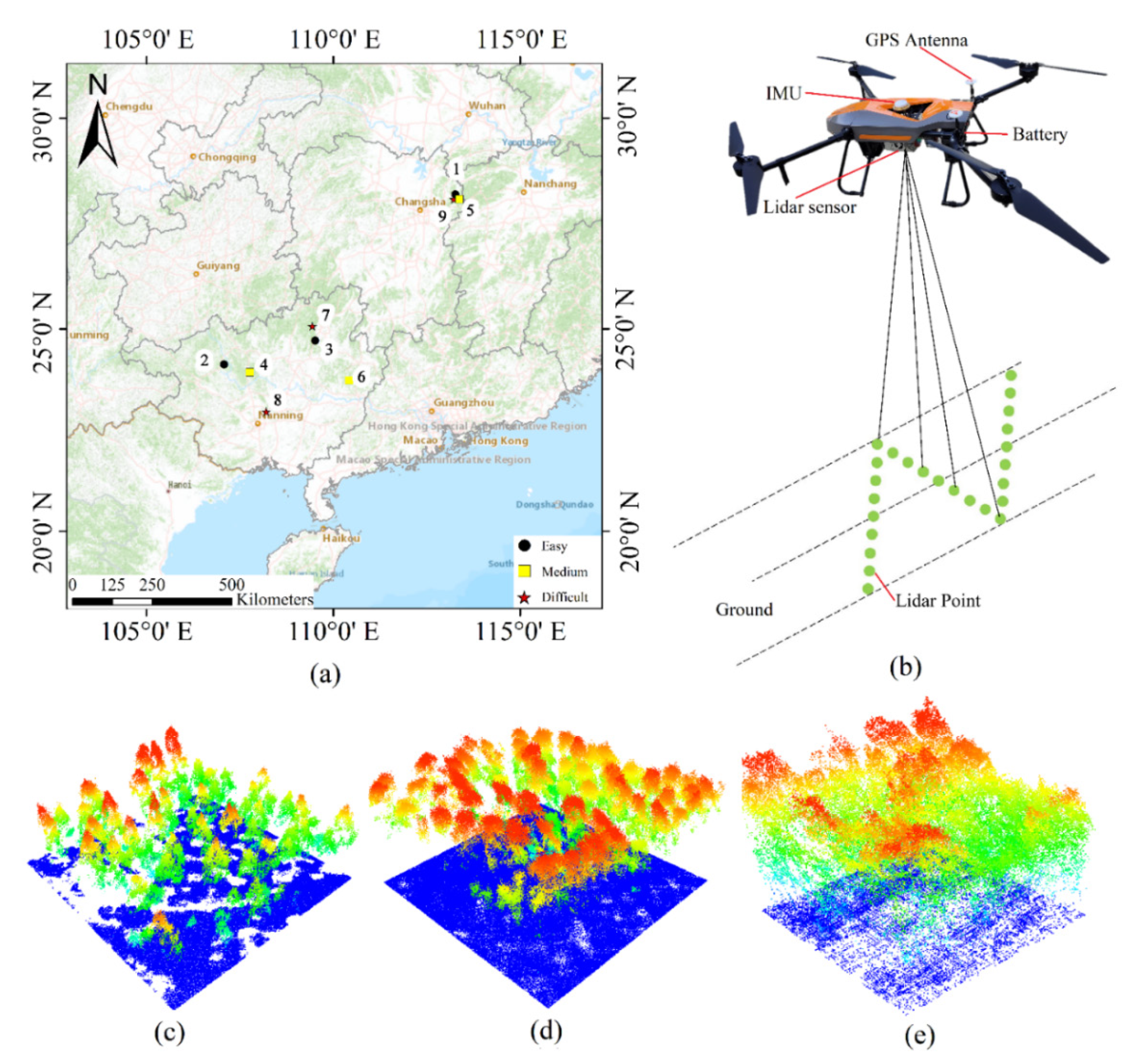
2.1. Study Area

Two study areas located in the subtropical monsoon climate zone in southern China were selected, as shown in Figure 1: (1) the Lutou Experimental Forest Farm of Central South University of Forestry Science and Technology in Yueyang, Hunan Province (113°51′~113°58′E and 28°31′~28°38′N), where the annual average temperature is 16.8 °C, the annual precipitation is approximately 1500 mm, the forest coverage rate is 94.2%, and the vegetation is mainly evergreen broad-leaved forest and coniferous forest, and (2) the Guangxi Zhuang Autonomous Region (104°28′~112°04′E and 20°54′~26°23′N), which has an annual average temperature of 20.7 °C and receives 1542.5 mm of rainfall on average each year. Under these favorable hydrothermal conditions, plants can grow year-round, and the growth of trees is 2~3 times the national average. Eucalyptus (Eucalyptus robusta Smith) and Chinese fir (Cunninghamia lanceolata) are the main species, followed by natural evergreen broad-leaved mixed forests that include Schima superba (Schima superba Gardn. et Champ.), Sweetgum (Liquidambar formosana Hance), Cyclobalanopsis glauca (Cyclobalanopsis glauca Thunb. Oerst.) and oriental oak (Quercus variabilis Bl.). The two study areas include five coniferous forest plots with Chinese fir and four broad-leaved forest plots with Eucalyptus, Schima superba, Sweetgum, etc. The first seven of these plots are artificial forests, and the last two are natural forests. All plots are mature forests, the average tree height is approximately 10 m, and the number of trees in each plot ranges from 14 to 108. The natural forest plots are coniferous and broad-leaved mixed forests, and there are some shrubs under the tree canopy. The forest types in the study areas are complex, making it very challenging to accurately segment individual trees.

2.2. Data Collection

2.2.1. Field Experiments

For validation purposes, nine square research plots of 25.82 m × 25.82 m (0.067 ha) were established. According to the number of trees, the complexity of tree arrangement, the mixing degree of tree species, and the complexity of the terrain, the forests were classified into three complexity categories, namely, ‘easy’, ‘medium’, and ‘difficult’, to represent different stand situations, which varied in terms of natural state, species and growth stages. These stands included both homogenous and heterogeneous forests. In the sample plots, each tree with a DBH greater than 5 cm was measured, and the structural parameters of each tree, such as its height, DBH, and crown size, were recorded; the results are shown in Table 1. The tree height was measured twice by a TruPulse 200 laser rangefinder, the average height was taken, and the measurement error was ignored. DBH was calculated by measuring the circumference of the trunk 1.3 m from the ground with a tape measure. A real-time kinematic (RTK) global positioning system (GPS) was used to locate and record the coordinates of each tree, and these data were used to evaluate the accuracy of the tree positions detected by the individual tree segmentation methods used in this study.

2.2.2. LiDAR Data

LiDAR point cloud data were obtained using the Shanghai Huace navigation BB-4 or DJI Matrix 600 UAV platform and a RIEGL VUX-1LR. The data were scanned in December 2020. Clear and cloudless weather was selected for data acquisition. Routes were planned and flight tests were performed in advance, and a vertical intersection route design was adopted. The UAV working mode and LiDAR sensor parameter settings were determined according to the fight altitude and elevation variations in the sample plot. Specifically, the flight altitude was 150 m, the flight belt interval was 70–100 m, the flight speed was 6 m/s, the emission frequency of the laser pulse was 300 kHz, the scanning angle was 140–180°, and the point cloud density was greater than 300 pts/m2. After acquisition, position and orientation system (POS) processing, aerial belt splicing, and data correction were performed to obtain the UAV-LiDAR point cloud data for the study area.

2.3. Data Models

The data models required by tree segmentation algorithms are generally NPC models and CHMs [23,24,25,26,27]. Therefore, it is necessary to preprocess the UAV-LiDAR point cloud data.

2.3.1. Data Preprocessing

Lidar 360 software was used for data preprocessing. First, a denoising method based on spatial distance was used to remove the noise caused by sensors, leaf-related factors, water vapor, etc. The algorithm determines whether a given point is a noisy point based on the average distance between the target point in the neighborhood and all other points [40]. The number of neighborhood points was set to 20, and the standard deviation multiple was set to 5. Then, improved progressive triangulated irregular network identification (IPTD) was used to classify ground points [41,42]. This algorithm generates a sparse triangulated irregular network through seed points and encrypts each layer through iterative processing until all the ground points are classified [24]. The key parameters of the algorithm in Lidar 360 software are the maximum terrain slope, iteration angle, and iteration distance, which were set to 60°, 10°, and 1 m, respectively. In the stand environment, non-ground points were treated as vegetation point clouds. Finally, an NPC and a CHM were obtained.

2.3.2. Normalized Point Cloud

An NPC is a new point cloud set obtained by subtracting the elevation value Z0i of the ground point closest to a given point in a plane projection from the elevation value Zi at that point [43]. The elevation value at the lowest point is 0, and the elevations at other points reflect the canopy height.

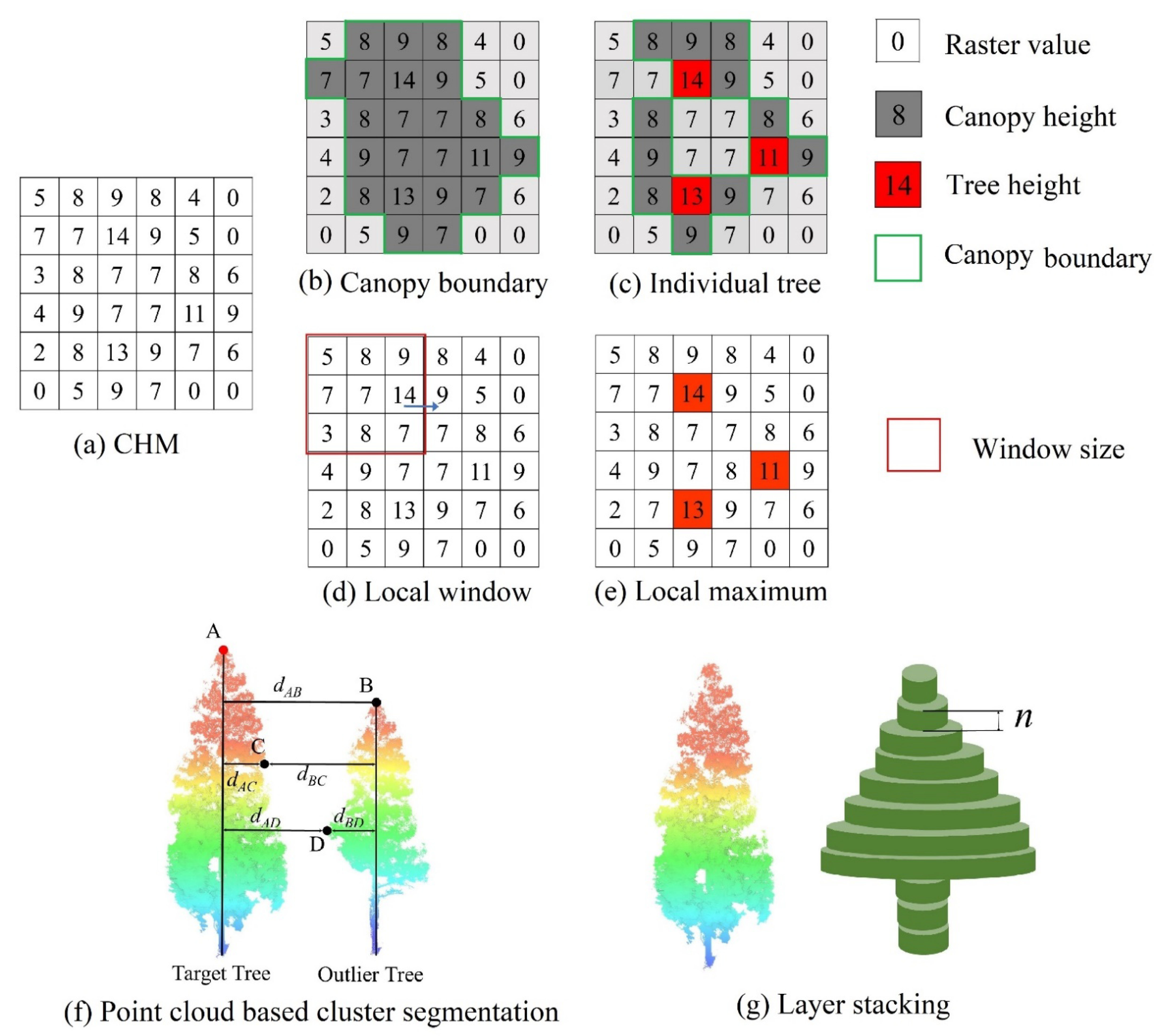
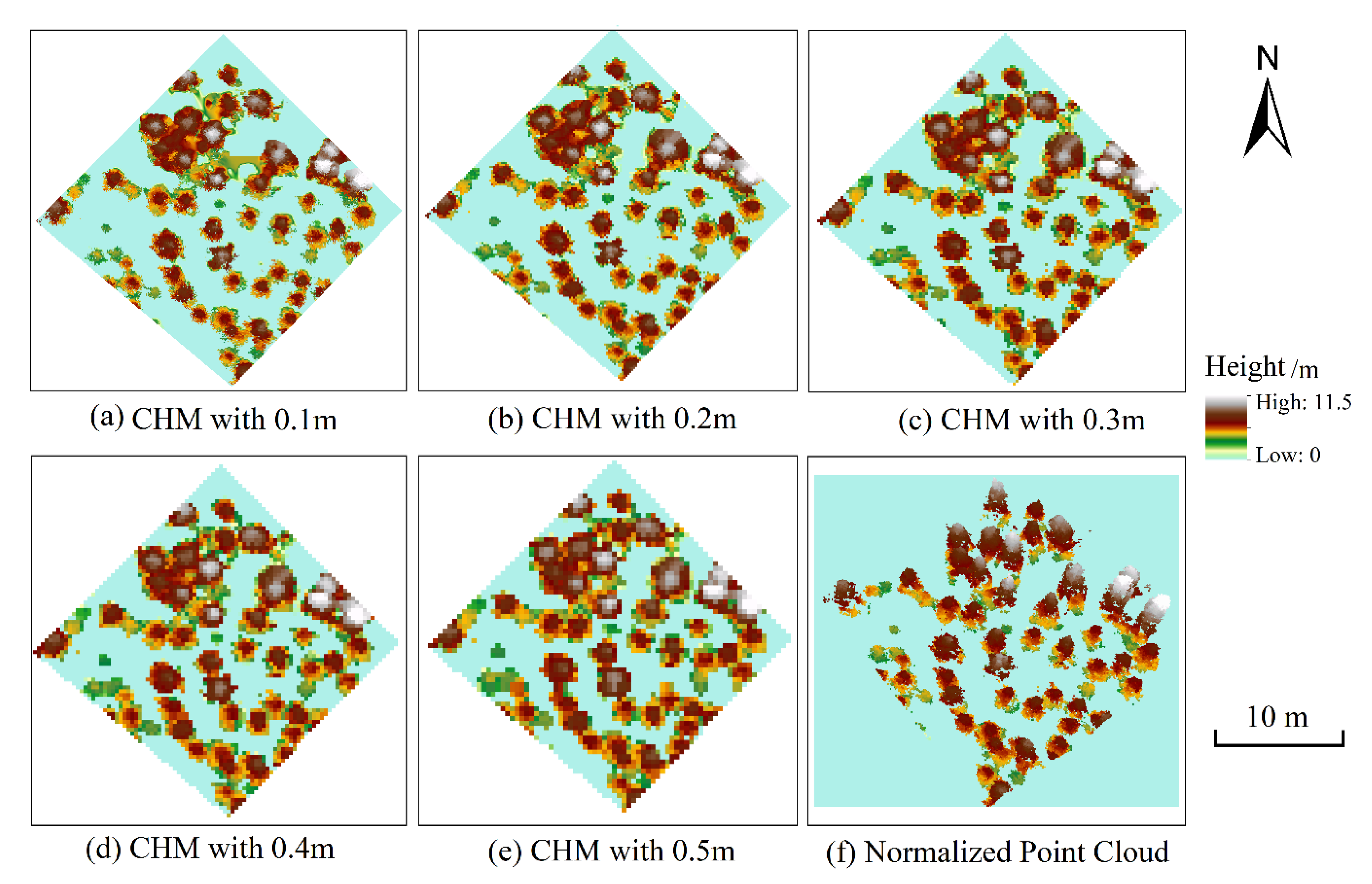
2.3.3. Canopy Height Model

A CHM contains the raster values of a digital elevation model (DEM) subtracted from the raster values of a digital surface model (DSM). A CHM is constructed by using inverse distance weighting (IDW) interpolation and ground point clouds [44,45,46] to generate a DEM, and a DSM is obtained by interpolating the laser point cloud of the first echo. The result is a direct expression of the distribution of the vegetation canopy height above the ground [47]. In this study, the CHM resolution was set to range from 0.1 m to 0.5 m. This method was used to explore the influence of the CHM resolution on the accuracy of individual tree segmentation.

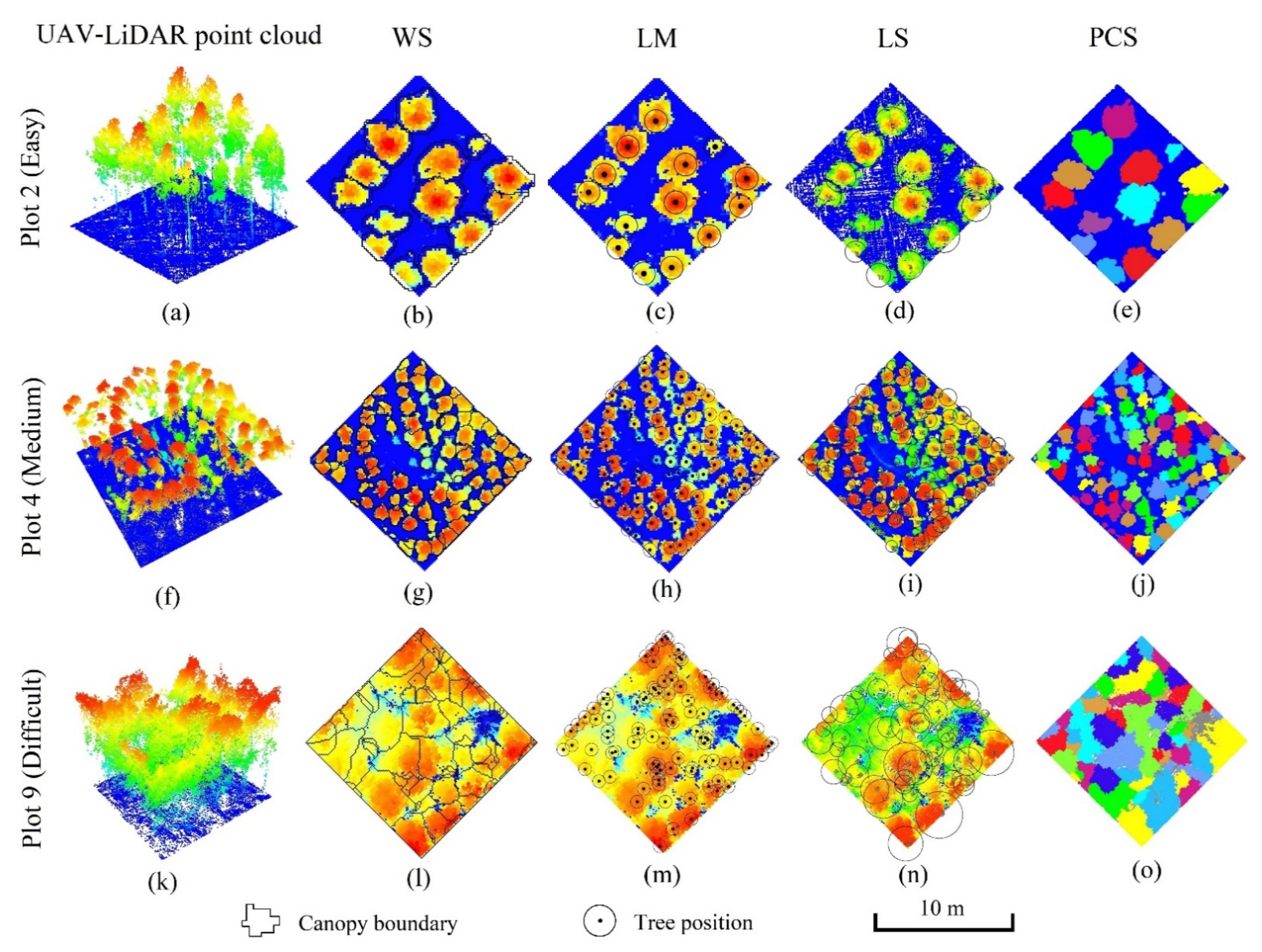
2.4. Individual Tree Segmentation

The individual tree segmentation methods employed in this study included the WA, (LM), PCS, and LS. The WA and LM are CHM-based segmentation methods, whereas PCS and LS are PCS-based algorithms. In this paper, we assessed the segmentation performance of the WA and LM segmentation algorithms at multiple CHM resolutions and evaluated the advantages of the CHM-based and NPC-based segmentation methods. We then explored the influences of the key parameters of the four different methods on the segmentation accuracy; these parameters include the minimum height (hmin) and the Gaussian smoothing factor (sigma) in the WA, the window size in the LM, the distance threshold in the PCS algorithm, and the layer thickness in LS.

2.4.1. Watershed Algorithm

The WA is an image segmentation algorithm that can sensitively recognize subtle changes in the gray level of a CHM and generate closed contour lines around target objects [24,48]. The formation of a watershed is based on the concept of simulating immersion. If an image is regarded as a forest canopy surface, the gray value of each pixel represents the canopy height at that point in the image. In Figure 2b,c, each local maximum is the high point of a tree, and the corresponding area of influence is called the catchment basin (individual tree canopy). The algorithm can automatically construct a barrier at watershed boundaries (canopy boundaries) to prevent water from two adjacent watersheds (tree models) from merging. Two important parameters of the algorithm are hmin and sigma. The minimum height is the threshold value of the minimum tree height range used for tree segmentation. If this value is less than hmin, the vegetation is not considered, and sigma affects the number of trees segmented. In this study, hmin was set to 2.1 m, which means that trees with a height below 2.1 m were not considered for segmentation. Sigma was set to the range of 0.5–2, and the optimal parameters were adjusted according to the type of plot.

2.4.2. Local Maximum Algorithm

When the value of a pixel in a grid in a given window is larger than the values of the surrounding pixels, the pixel is defined as the local maximum [49,50]. The specific steps are as follows, as shown in Figure 2d,e. First, a CHM with an appropriate raster resolution is created. Then, the local maximum is found from the CHM in a given size window, and the window is moved until all the maximum values are detected. If the local maximum is higher than the minimum tree height, the tree is considered to have been detected. The raster resolution of the CHM and the window size (z) are affected by the forest conditions and tree crown size. When the resolution is high, many small trees are not detected, and when the window size is large, two or more trees in close proximity are grouped as one. In this study, the window size was set to range from 1 × 1 to 9 × 9 pixels.

2.4.3. Point Cloud-Based Cluster Segmentation

PCS is an algorithm that combines regional growth and threshold judgment to segment individual tree point clouds from standpoint clouds [25]. The algorithm mainly considers that there is a certain Euclidean distance between two trees, especially at the tops of trees, within the tree point cloud. Assuming that the highest point in a tree point cloud is the tree vertex, the tree vertex can be used as the seed point to establish the corresponding regional growth and separate individual trees; this process is iterative. Each segmentation involves regional growth from top to bottom, and the distance threshold (D) is determined. In Figure 2f, point A is the highest point, so point A is regarded as the top of the target tree. Next, the points lower than A are successively classified. First, point B is classified as an outlier tree because the spacing dAB is greater than D. Then, we set point C, and the spacing dAC of point C is less than the critical value. By comparison with the categories of point A and point B, the category of point C is set to that of the target tree because dAC is less than dBC. By comparison with points B and C, point D is classified as an outlier tree. If the distance at a point is greater than the threshold interval, the point is considered the vertex of another tree. If the point is within the interval threshold, then the point is grouped with the existing split tree. In this study, we set the distance threshold within 0.5–3 m according to the average spacing of trees in each plot.

2.4.4. Layer Stacking

LS is a segmentation method based on NPC data. The point cloud of an entire stand is sliced at a given interval, the tree position is identified in each layer, and the results from all layers are merged to produce a representative tree boundary [34]. The basic idea of the algorithm is as follows. (1) Point cloud layering. We started from 0.5 m above the ground and used 1 m as the layering interval until the highest point (tree top) was reached, as shown in Figure 2g. (2) Point cloud clustering. We used K-means clustering to cluster the sliced point cloud data to the nearest seed point and iteratively repeated this process until the position of the seed point did not change. In doing so, we sought to obtain tree seed points for each layer. (3) Build polygons. In each layer, we constructed a Thiessen polygon by using tree seed points. (4) Overlapping and merging. We stacked the Thiessen polygons of each layer to generate a large number of rasterized overlapping polygons. An area of considerable overlap is a high-density area in the tree crown, indicating the presence of an individual tree in the polygonal overlapping area. The layer thickness (n) used in the LS algorithm influences the detection ability of this method for trees at different forest levels.

2.5. Accuracy Evaluation

The four individual tree segmentation algorithms were implemented using Python software. To evaluate the performance and sensitivity of the four methods, the individual tree segmentation results were compared with the field-observed tree heights and positions using three indices: the detection rate (Equation (1)), accuracy rate (Equation (2)), and overall accuracy (Equation (3)) [35,51,52]:
r = N c N c + N m ,
p = N c N c + N o ,
F = 2 r p r + p ,
where r represents the detection rate of an individual tree; p represents the accuracy rate for an individual tree; F is calculated from r and p; and Nc, Nm, and No represent the numbers of correct segmentations, missing segmentations and over-segmentations, respectively. F was calculated in SPSS software. A high F indicates an accurate individual tree detection result.
The coefficient of determination (R2) (Equation (4)), root mean square error (RMSE) (Equation (5)), and RMSE% between the measured tree height and extracted tree height were calculated to evaluate the tree height accuracy:
R 2 = i = 1 n ( x i x i ¯ ) ( X i X i ¯ ) i = 1 n ( x i x i ¯ ) 2 i = 1 n ( X i X i ¯ ) 2 ,
R M S E = i = 1 n ( X i x ) 2 n ,
where n is the number of correctly segmented individual trees; Xi represents the heights of the individual segmented trees; X ¯ i represents the mean height of the individual trees, xi represents the measured heights of the individual segmented trees, and x ¯ i represents the mean value of the measured heights of the individual segmented trees.

3. Results

3.1. Data Model Generation

The NPC and CHM obtained from the UAV-LiDAR point cloud are shown for plot 6 in Figure 3. Additionally, panels (a)–(e) plot the results at raster resolutions of 0.1 m × 0.1 m, 0.2 m × 0.2 m, 0.3 m × 0.3 m, 0.4 m × 0.4 m, and 0.5 m × 0.5 m, respectively, and (f) is the NPC result. With increasing raster resolution, the CHM details are gradually ignored. When the resolution decreases to 0.1 m, the jagged crown boundaries and low shrubs in local areas affect the accuracy of individual tree segmentation. In contrast, the NPC approach retains the complete three-dimensional information for trees and removes the influence of terrain.

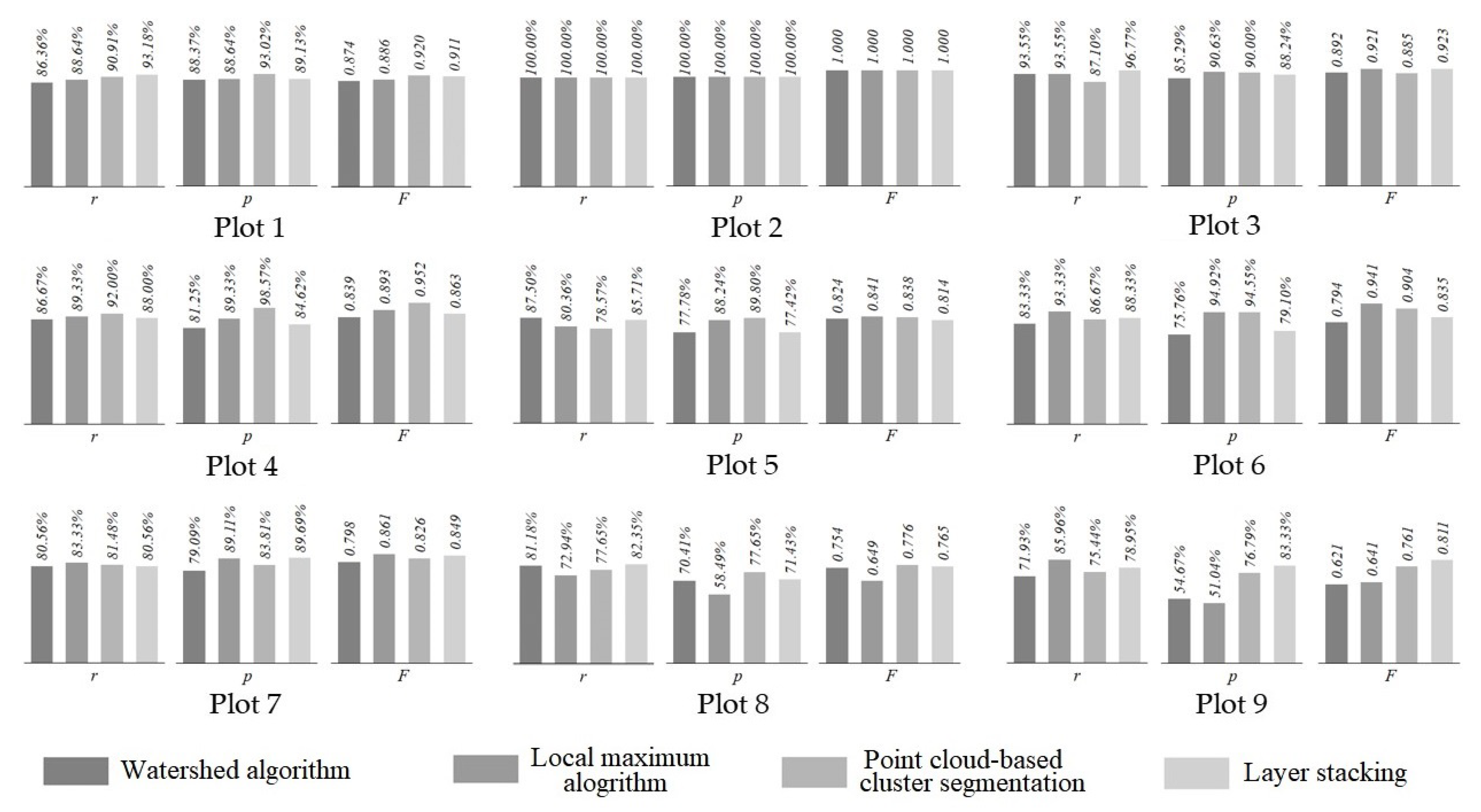
3.2. Accuracy of Individual Tree Detection

The segmentation effects of the four individual tree segmentation methods for some sample plots are shown in Figure 4; plot 2 is classified as ‘easy’, plot 4 is classified as ‘medium’, and plot 9 is classified as ‘difficult’. In plot 2, the four individual tree segmentation methods accurately segmented all 14 trees. The WA completely divided the boundary of the tree crown in the CHM. The PCS approach segmented the standing forest point cloud data into individual tree point clouds and visualized them with different colors according to the tree IDs. The LM and LS algorithms also accurately identified the positions of tree tops. In plot 4, 75 trees in the sample plot were Eucalyptus trees, and the crown area of individual trees was small. Among the four individual tree segmentation methods, the WA undersegmented some adjacent trees, and the LM and LS methods yielded satisfactory segmentation results for the tree positions. The individual tree point cloud segmented by the PCS method also accurately depicted the actual sizes of individual trees. In plot 9, due to the mixture of broad-leaved tree species such as Cyclobalanopsis glauca and Liquidambar formosana, the segmentation ability of WA was obviously insufficient; notably, this method could segment only some trees with large crowns, while the segmentation effect for small trees was relatively poor. In areas of broad-leaved trees with large canopies, multiple trees with small canopies were detected by the LM. Moreover, the size of individual tree point clouds segmented by the PCS method was relatively uniform, meaning that the actual uneven distribution of tree sizes in the sample plot was not accurately expressed. Compared with the other three methods, the LS method achieved the best segmentation result.
The accuracy was evaluated by matching the individual tree segmentation results obtained with the four segmentation methods in the nine sample plots with the measured position data for each tree in the sample plots, as shown in Figure 5. To solve the problem in which the top of a tree was inconsistent with the field-measured position of its trunk, we established a buffer zone of 1–2 m around the trunk to match the detected position of the individual tree using segmentation methods. The experimental results show that among the three easy plots, the detection rate (r) and accuracy rate (p) were greater than 86.36% and 85.29%, respectively, and F was greater than 0.874. In plot 2, there were 14 Chinese fir trees, r and p were both 100%, and F was 1. Accordingly, the four methods yielded accurate segmentation results. Among the three medium plots, r varied from 78.57% to 93.33%, p ranged from 75.76% to 98.57%, and F varied from 0.794 to 0.952. The PCS method yielded the highest accuracy in plot 4, while the WA yielded the lowest accuracy in plot 6. Among the three difficult plots, the highest r and p values for the four methods were 85.96% and 89.69%, respectively, and they were obtained for plot 9 using the LM and for plot 7 using the LS algorithm. The lowest corresponding values were 71.93% and 51.04%, which were obtained for plot 9 using the WA and LM, respectively. F varied from 0.621 to 0.861, with the best result obtained for plot 7 and the worst result obtained for plot 9.

3.3. Accuracy of Tree Height Parameters

A linear relation between the extracted tree height and measured tree height was established according to the types of plots. R2 and RMSE were calculated between the extracted tree height and the measured tree height, and the calculation results are shown in Table 2.
The experimental results indicate that different segmentation methods exhibit notable differences in the segmentation accuracy among the three types of plots; however, the difference between the accuracy of the segmentation results and the tree height extraction accuracy calculated after actual matching is minimal. The difference between the maximum and minimum values of R2 is within 0.05, and the difference in RMSE is less than 0.19 m. These findings suggest that the tree height extraction results of the four methods are stable and that the four methods can be applied to extract the individual tree height parameters involving UAV-LiDAR point clouds.

3.4. Sensitivity Analysis of the Four Methods

To explore the influence of the key parameters of the four different methods on the segmentation accuracy for the three types of plots, the sigma factor in the WA, the window size in the LM, the distance threshold in the PCS algorithm, and the layer thickness in the LS algorithm were adjusted, and the sensitivity differences among the four segmentation methods were analyzed.

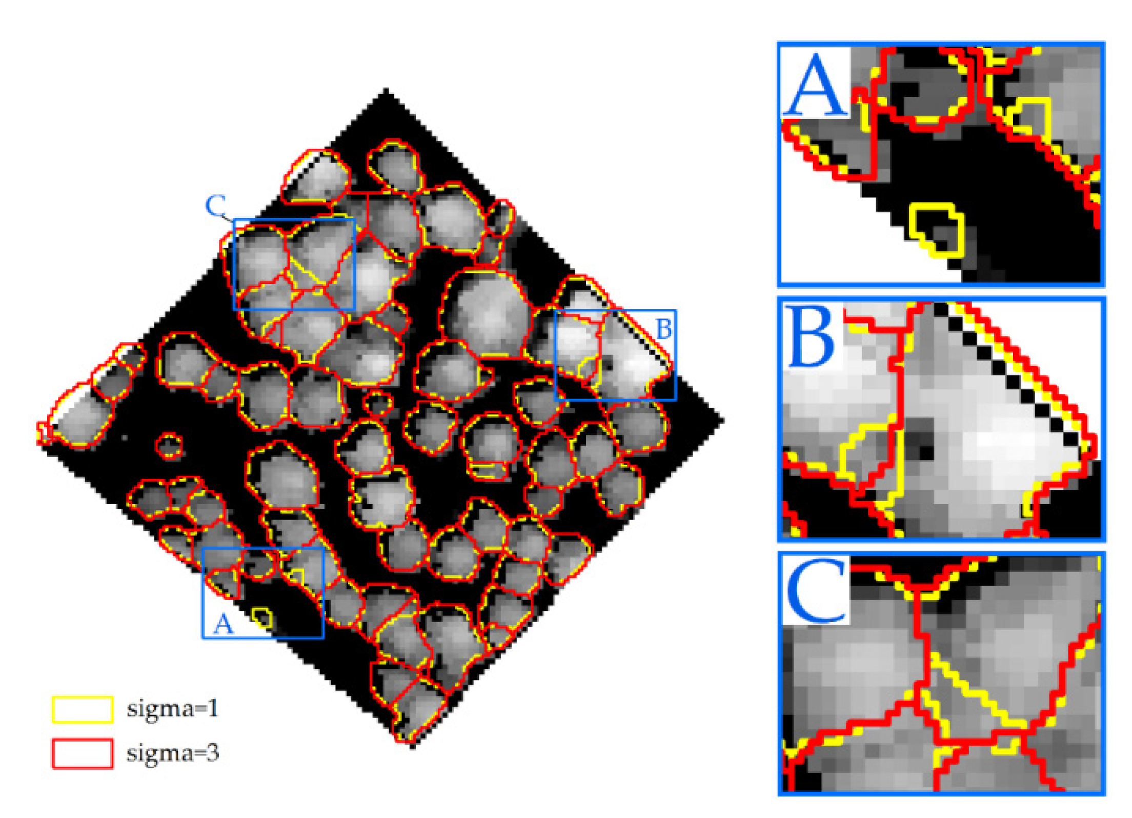
3.4.1. Watershed Algorithm

The segmentation results of the WA with different sigma values are shown for plot 6 in Figure 6. In region A, when sigma = 1, the small trees that are not divided when sigma = 3 can be divided. In region B, the crown boundary details are most obvious when sigma = 1. In region C, when sigma = 1, a complete tree in the upper right corner is divided into two trees. Therefore, the smaller the sigma value is, the finer the segmentation of crown boundaries. In contrast, the larger the sigma value is, the smaller the number of segmentations; additionally, low-level trees are insufficiently segmented, resulting in a large average forest tree height.

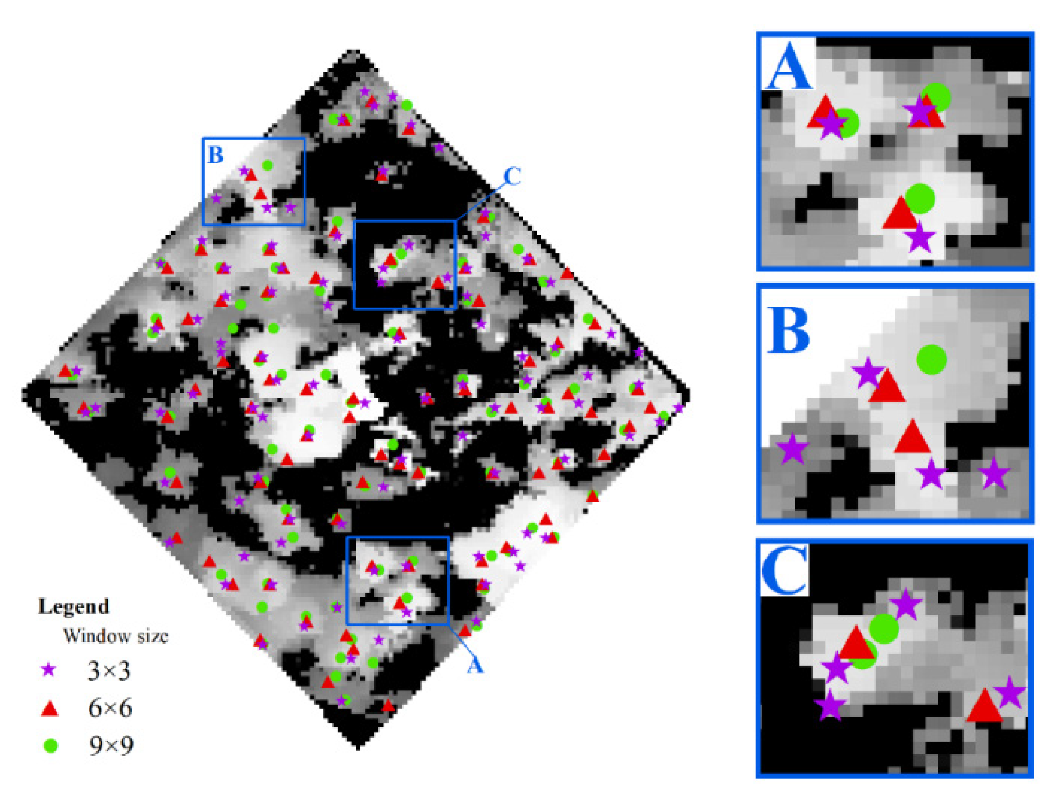
3.4.2. Local Maximum Algorithm

Different window sizes (z) were set for plot 8, and the segmentation results of the LM were obtained, as shown in Figure 7. Eighty-five Eucalyptus trees were measured in the plot, and z was set to 3 × 3, 6 × 6, and 9 × 9. The number of individual trees is 95, 82, and 75 in plot 8. In area A, three trees with obvious boundaries are accurately detected at all window sizes. In areas B and C, the z value for a window size of 3 × 3 is significantly larger than the z values for window sizes of 6 × 6 and 9 × 9. The results indicate that the larger z is, the weaker the ability of the model to detect individual trees and the more prone the approach to under-segmentation. In contrast, the smaller z is, the better the individual tree detection results; however, over-segmentation can easily occur.

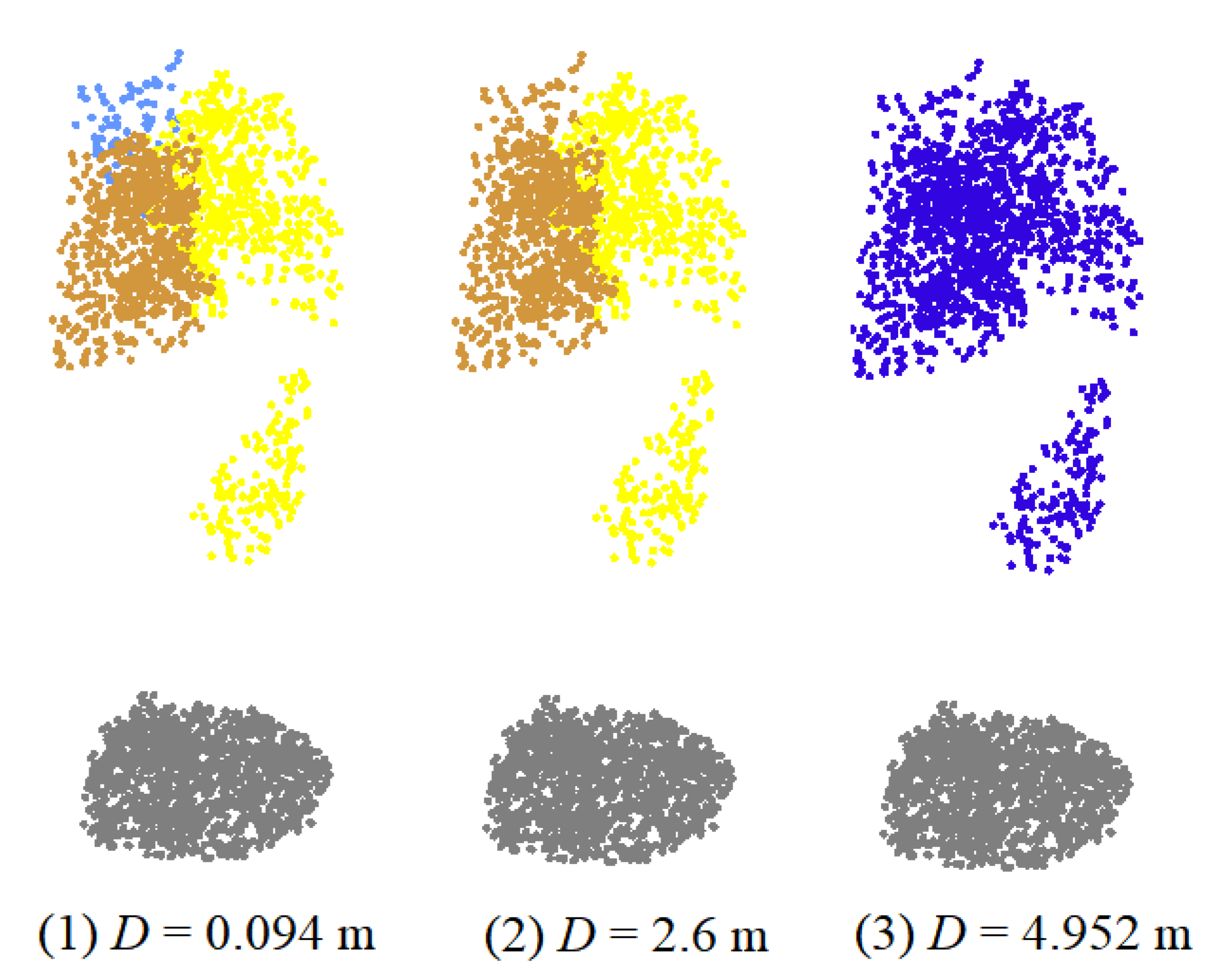
3.4.3. Point Cloud-Based Cluster Segmentation

The distance threshold (D) in PCS is the key parameter that influences individual tree segmentation. Different D values were set for plot 1, plot 4, and plot 8, and the individual tree segmentation results obtained using the PCS method are presented in Table 3. The results are based on the maximum, average, and minimum values of the crown radius of the plot. In different types of plots, the number of individual tree segmentations decreases with an increasing distance threshold, and these factors are negatively correlated. When D is set as the average crown radius, the F values of the three plots reach maxima of 0.851, 0.848, and 0.776. A comparison among the PCS segmentation details for different D values was performed for plot 4, as shown in Figure 8. There are two adjacent Eucalyptus trees in this plot, and over-segmentation occurs when D is set to the minimum crown radius; when D is set to the maximum crown radius, three trees are combined into one. However, when D is set to the average crown radius, the three trees are segmented correctly.

3.4.4. Layer Stacking

Similarly, we used different layer thicknesses in the LS method for plot 1, plot 4, and plot 8, and the segmentation results are shown in Table 4. The layer thickness (n) was set as 0.5 m, 1 m, and 2 m. When n = 1 m, the optimal segmentation results are obtained for the three plots. The segmentation results for n = 0.5 m and n = 1 m are similar, whereas when n = 2 m, the number of individual trees detected is too large, and the accuracy is relatively poor.

4. Discussion

4.1. Data Model

We found that the segmentation results of the CHM and NPC data models are characterized by similar detection rates (r), with no obvious difference. Kaartinen et al. [53] summarized and compared a variety of methods, including a variety of single tree extraction methods based on grid CHM and clustering segmentation methods based on point clouds. The results showed that the extraction accuracy of all single tree extraction methods for the heights of individual trees was better than 0.5 m, which is consistent with the accuracy observed in this research. In terms of the accuracy rate (p), the individual tree segmentation methods based on NPCs perform better than those based on CHMs, and the differences between the two approaches were obvious in a difficult broad-leaved heterogeneous forest. In the high-forest-density plots, the effect of individual tree segmentation based on NPCs was better than that based on a CHM. Because a CHM is a two-dimensional raster model that involves the projection and interpolation of point cloud data, more data conversion steps are required than are needed for an NPC; therefore, a CHM achieves a comparatively worse segmentation performance. Yang et al. [54] also reached this conclusion and showed that the overall accuracies of PCS and LS methods are higher than those of methods based on CHMs. With improvements in the airborne LiDAR point cloud data density and quality, individual tree segmentation based on NPC will become an even better choice.

4.2. Method Sensitivity

Analyzing the sensitivities of different algorithm parameter settings is critical for selecting the appropriate segmentation method. The WA was suitable for individual tree segmentation in the CHM generated by low-density LiDAR point cloud interpolation. However, the results were significantly affected by the interpolation algorithm and grid resolution, and the accuracy was low. When the resolution is too low or too high, a CHM generated by interpolation does not match the actual size of the tree crown: when the resolution is too low, there are many convex and concave CHMs, resulting in over-segmentation; if the resolution is too high, the CHMs are too smooth, resulting in leakage, which is consistent with the research of Sokolova et al. [55]. Alternatively, the LM can accurately explore the positions of tree tops, which is suitable for homogeneous forests with regular crown shapes and neat arrangements of trees. To some extent, our results support the conclusions of Peuhkurinen et al. [56], who suggested that individual tree segmentation is affected by the number of trees, the size of trees, the arrangement of tree positions, the canopy coverage, and changes in the tree size. Nevertheless, if the distance threshold of PCS is too large or too small, insufficient, or excessive segmentation will occur. The optimal distance threshold should equal the average canopy radius of the plot. Our results are also consistent with those of Li et al. [32], who showed that the uncertainty in the use of the PCS algorithm for individual tree segmentation originates mainly from the distance threshold. In sparse forests with a large tree spacing, a relatively large threshold can be used to isolate trees. In contrast, it is difficult to determine the appropriate threshold in dense forests, so additional classification rules should be combined to obtain the optimal results. Furthermore, the LS method can effectively achieve the individual tree segmentation of multilayer forests, and using the appropriate layer thickness (n) can improve the segmentation accuracy. Ayrey et al. [34] showed that because the crown edges of Pinus strobus overlap more than the center of the tree, a single tree can be divided into many parts. Especially in broad-leaved forests with more shrubs under the trees, the LS algorithm is particularly prone to clustering errors in slices [55], and the results from this study further support this. Overall, the adjustment of key parameters in each individual tree segmentation method has a considerable impact on the accuracy of tree detection. The most suitable parameters vary based on the plot considered and forest type.

4.3. Uncertainty Related to the Forest Type

The forest type is influenced mainly by the forest density, species types, degree of species mixing, tree arrangement, and other factors. The variation in forest density was not the predominant influencing factor on the accuracy of individual tree segmentation, although previous studies have always emphasized the influence of tree density [24,57,58]. Instead, this study found that forest homogeneity or heterogeneity was the most important factor. F = 0.92 was obtained for the segmentation result among the seven plots with homogeneous tree species; this F value is much larger than that obtained for the two plots with heterogeneous tree species. The tree density in many of these homogeneous forests was significantly higher than that in the heterogeneous forests. In addition, the uncertainty related to the tree species in the plot was the main factor that influenced the selection of the best segmentation method. The results reported by Mohan et al. [52] and Wang et al. [57] are consistent with our findings, indicating that the accuracy of tree detection is affected by the tree species and crown shape of adjacent trees. For Chinese fir and Eucalyptus species with obvious peaks, the segmentation accuracy of the LM was high, and for broad-leaved species such as Cyclobalanopsis, over-segmentation easily occurred, resulting in poor accuracy. The LS method performed best in the segmentation of deciduous broad-leaved forests [55]. The accuracy of the individual tree segmentation algorithm based on NPC data depends strongly on the tree arrangement obtained from airborne LiDAR. For example, in plantation plots 5 and 6 with high forest densities and close tree spacing, the PCS method produced under-segmented results, whereas, for plots with regular arrangements of trees and sufficient spacing, high-precision segmentation results were obtained. This result is consistent with the conclusion of Li et al. [33] regarding the distance threshold in the PCS algorithm. In addition, Larjavaara et al. [59], Butt et al. [60], and Krause et al. [61] considered the influence of the errors of tree measurements in the field. In this paper, we directly used the field data as a reference to verify the accuracy of extracted tree heights.

5. Conclusions

In this research, we used UAV-LiDAR point cloud data to generate NPCs and a CHMs for multiple subtropical types of forest plots and compared and analyzed the performance and accuracy of four segmentation methods. On this basis, we discussed the sensitivity of the key parameters of each segmentation method, thus providing a basis for accurate forestry measurements from UAV-LiDAR products.
(1) Compared with the CHM-based methods, the NPC-based methods exhibited better performance in individual tree segmentation. Among the nine plots considered in this study, the individual tree segmentation results of the former methods exhibited an average detection rate r = 81.28%, an average accuracy rate p = 86.58%, and an average overall accuracy F = 0.835. In contrast, the results of the NPC-based methods exhibited an average detection rate r = 87.06%, an average accuracy rate p = 86.87%, and an average overall accuracy F = 0.869. These findings suggest that the r values of individual trees are lower for the CHM-based methods results than for the NPC-based methods due to the limited pixel resolution of CHM rasters. Moreover, while the p values of the two datasets were similar, and NPC methods yielded a higher overall accuracy F.
(2) By comparing the parameter sensitivities of the four segmentation methods, we concluded that the key parameters of the segmentation method and segmentation accuracy are not consistently related, and the key parameters depend on the plot conditions. Overall, in terms of the detection capability, the sigma value of the WA, the window size (z) of the LM, and the distance threshold (D) in PCS are negatively correlated with the detection rate r; conversely, the layer thickness (n) in LS exhibits a positive correlation with r. However, in terms of the overall accuracy of segmentation F, the optimal sigma and z values depend on the individual tree arrangement in a forest plot, the optimal D is affected by the average crown radius, and the optimal n is influenced by the tree species present and tree stratification in a plot. Therefore, these results are important for selecting and setting the key parameters of UAV-LiDAR-based methods for individual tree segmentation to accurately obtain forest structure information.
(3) Our extensive experiments showed that different individual tree segmentation methods can provide excellent performance for different specific types of forest plots. In addition, the forest type and complexity have notable impacts on the accuracy of individual tree segmentation. Specifically, the WA and LM were minimally advantageous for individual tree segmentation using high-density point cloud data from UAV-LiDAR. Alternatively, the PCS method can be used as the preferred scheme for the individual tree segmentation of UAV-LiDAR point cloud data, and its segmentation performance was better in many types of forests. LS should be used as a supplement for individual tree segmentation in multilayer forests and extremely complex heterogeneous forests.
Ultimately, this study provides an efficient solution for precisely surveying and monitoring forest resources of multiple forest types. This study can be applied to ecological research to study the acquisition of regional canopy heights and vegetation indices.

Author Contributions

Conceptualization and methodology, H.S. and K.M.; validation, K.M. and F.J.; formal analysis, K.M., F.J. and J.Y.; investigation, K.M., Z.C., W.T. and Z.D.; draft, K.M., L.F. and H.S.; supervision, L.F. and H.S.; review, editing, and revision, K.M., J.Y. and H.S.; funding acquisition, K.M. and H.S. All authors have read and agreed to the published version of the manuscript.

Funding

This research was funded by the National Natural Science Foundation of China (No: 31971578); the Scientific Research Fund of Changsha Science and Technology Bureau (No: kq2004095); the Scientific Research Fund of Hunan Provincial Education Department (No: 17A225); and the Hunan Province Innovation Foundation for Post-graduates (No: CX20200705).

Institutional Review Board Statement

Not applicable.

Informed Consent Statement

Not applicable.

Data Availability Statement

The data presented in this study are available on request from the corresponding author.

Acknowledgments

The authors would like to thank the Central South Inventory and Planning Institute of the National Forestry and Grassland Administration for their help with the fieldwork. The authors also thank Shanghai Huace Navigation Technology Ltd. for the LiDAR data.

Conflicts of Interest

The authors declare no conflict of interest.

References

  1. FAO Voluntary Guidelines on National Forest Monitoring; Food and Agriculture Organization of the United Nations: Rome, Italy, 2017; ISBN 978-92-5-109619-2.
  2. Duncanson, L.; Armston, J.; Disney, M.; Avitabile, V.; Barbier, N.; Calders, K.; Carter, S.; Chave, J.; Herold, M.; Crowther, T.W.; et al. The importance of consistent global forest aboveground biomass product validation. Surv. Geophys. 2019, 40, 979–999. [Google Scholar] [CrossRef] [PubMed] [Green Version]
  3. Zhao, P.; Lu, D.; Wang, G.; Liu, L.; Li, D.; Zhu, J.; Yu, S. Forest aboveground biomass estimation in Zhejiang Province using the integration of Landsat TM and ALOS PALSAR data. Int. J. Appl. Earth Obs. 2016, 53, 1–15. [Google Scholar] [CrossRef]
  4. Rex, F.E.; Silva, C.A.; Dalla Corte, A.P.; Klauberg, C.; Mohan, M.; Cardil, A.; Silva, V.S.D.; Almeida, D.R.A.D.; Garcia, M.; Broadbent, E.N.; et al. Comparison of Statistical Modelling Approaches for Estimating Tropical Forest Aboveground Biomass Stock and Reporting Their Changes in Low-Intensity Logging Areas Using Multi-Temporal LiDAR Data. Remote Sens. 2020, 12, 1498. [Google Scholar] [CrossRef]
  5. Herold, M.; Carter, S.; Espejo, A.B.; Jonckheere, I.; Lucas, R.; McRoberts, R.E.; Næsset, E.; Nightingale, J.; Petersen, R.; Reiche, J. The role and need for space-based Forest biomass-related measurements in environmental management and policy. Surv. Geophys. 2019, 40, 757–778. [Google Scholar] [CrossRef] [Green Version]
  6. Magnussen, S.; Nord-Larsen, T.; Riis-Nielsen, T. Lidar supported estimators of wood volume and above ground biomass from the Danish national forest inventory (2012–2016). Remote Sens. Environ. 2018, 211, 146–153. [Google Scholar] [CrossRef]
  7. Hyyppä, J.; Litkey, P.; Kaartinen, H.; Vastaranta, M.; Holopainen, M. Single-Sensor Solution to Tree Species Classification Using Multispectral Airborne Laser Scanning. Remote Sens. 2017, 9, 108. [Google Scholar]
  8. Hamraz, H.; Contreras, M.A.; Zhang, J. A robust approach for tree segmentation in deciduous forests using small-footprint airborne LiDAR data. Int. J. Appl. Earth Obs. Geoinf. 2016, 52, 532–541. [Google Scholar] [CrossRef] [Green Version]
  9. Roise, J.P.; Harnish, K.; Mohan, M.; Scolforo, H.; Chung, J.; Kanieski, B.; Catts, G.P.; McCarter, J.B.; Posse, J.; Shen, T. Valuation and production possibilities on a working forest using multi-objective programming, Woodstock, timber NPV, and carbon storage and sequestration. Scand. J. Res. 2016, 31, 674–680. [Google Scholar] [CrossRef]
  10. Ke, Y.; Quackenbush, L.J. A review of methods for automatic individual tree crown detection and delineation from passive remote sensing. Int. J. Remote Sens. 2011, 32, 4725–4747. [Google Scholar] [CrossRef]
  11. Lu, D.; Chen, Q.; Wang, G.; Liu, L.; Li, G.; Moran, E. A survey of remote sensing-based aboveground biomass estimation methods in forest ecosystems. Int. J. Digit. Earth. 2014, 9, 63–105. [Google Scholar] [CrossRef]
  12. Song, C. Optical remote sensing of forest leaf area index and biomass. Prog. Phys. Geog. 2013, 37, 98–113. [Google Scholar] [CrossRef]
  13. Stavros, E.N.; Schimel, D.; Pavlick, R.; Serbin, S.; Swann, A.; Duncanson, L.; Fisher, J.B.; Fassnacht, F.; Ustin, S.; Dubayah, R.; et al. ISS observations offer insights into plant function. Nat. Ecol. Evol. 2017, 1, 194. [Google Scholar] [CrossRef]
  14. Berninger, A.; Lohberger, S.; Stängel, M.; Siegert, F. SAR-based estimation of above-ground biomass and its changes in tropical forests of Kalimantan using L-and C-Band. Remote Sens. 2018, 10, 831. [Google Scholar] [CrossRef] [Green Version]
  15. Blomberg, E.; Ferro-Famil, L.; Soja, M.; Ulander, L.M.; Tebaldini, S. Forest biomass retrieval from l-band sar using tomographic ground backscatter removal. IEEE Geo. Remote Sens. Lett. 2018, 15, 1030–1034. [Google Scholar] [CrossRef]
  16. Zhen, Z.; Quackenbush, L.J.; Stehman, S.V.; Zhang, L. Agent-based region growing for individual tree crown delineation from airborne laser scanning (ALS) data. Int. J. Remote Sens. 2015, 36, 1965–1993. [Google Scholar] [CrossRef]
  17. Kato, A.; Moskal, L.M.; Schiess, P.; Swanson, M.E.; Calhoun, D.; Stuetzle, W. Capturing tree crown formation through implicit surface reconstruction using airborne lidar data. Remote Sens. Environ. 2009, 113, 1148–1162. [Google Scholar] [CrossRef]
  18. Hancock, S.; Armston, J.; Hofton, M.; Sun, X.; Tang, H.; Duncanson, L.I.; Kellner, J.R.; Dubayah, R. The GEDI simulator: A large-footprint waveform lidar simulator for calibration and validation of spaceborne missions. Earth Space Sci. 2018, 6, 294–310. [Google Scholar] [CrossRef]
  19. Kellner, J.R.; Armston, J.; Birrer, M.; Cushman, K.C.; Duncanson, L.; Eck, C.; Falleger, C.; Imbach, B.; Král, K.; Krůček, M.; et al. New Opportunities for Forest Remote Sensing Through Ultra-High-Density Drone Lidar. Surv. Geophy 2019, 40, 959–977. [Google Scholar] [CrossRef] [Green Version]
  20. Disney, M.I.; Vicari, M.B.; Burt, A.; Calders, K.; Lewis, S.L.; Raumonen, P.; Wilkes, P. Weighing trees with lasers: Advances, challenges and opportunities. Interface Focus. 2018, 8, 2. [Google Scholar] [CrossRef] [PubMed] [Green Version]
  21. Almeida, A.; Gonçalves, F.; Silva, G.; Mendonça, A.; Gonzaga, M.; Silva, J.; Souza, R.; Milk, I.; Neves, K.; Boeno, M.; et al. Individual Tree Detection and Qualitative Inventory of a Eucalyptus sp. Stand Using UAV Photogrammetry Data. Remote Sens. 2021, 13, 3655. [Google Scholar] [CrossRef]
  22. Hu, X.; Chen, W.; Xu, W. Adaptive Mean Shift-Based Identification ofIndividual Trees Using Airborne LiDAR Data. Remote Sens. 2017, 9, 148. [Google Scholar] [CrossRef] [Green Version]
  23. MA, K.; Xiong, Y.; Jiang, F.; Chen, S.; Sun, H. A Novel Vegetation Point Cloud Density Tree-Segmentation Model for Overlapping Crowns Using UAV LiDAR. Remote Sens. 2021, 13, 1442. [Google Scholar] [CrossRef]
  24. Lu, X.; Guo, Q.; Li, W.; Flanagan, J. A bottom-up approach to segment individual deciduous trees using leaf-off lidar point cloud data. ISPRS J. Photogramm. Remote Sens. 2014, 94, 1–12. [Google Scholar] [CrossRef]
  25. Wang, L.; Gong, P.; Biging, G.S. Individual Tree-Crown Delineation and Treetop Detection in High-Spatial-Resolution Aerial Imagery. Photogramm. Eng. Remote Sens. 2004, 70, 351–357. [Google Scholar] [CrossRef] [Green Version]
  26. Gougeon, F.A. A Crown-Following Approach to the Automatic Delineation of Individual Tree Crowns in High Spatial Resolution Aerial Images. Can. J. Remote Sens. 1995, 21, 274–284. [Google Scholar] [CrossRef]
  27. Vauhkonen, J.; Ene, L.; Gupta, S.; Heinzel, J.; Holmgren, J.; Pitkänen, J.; Solberg, S.; Wang, Y.; Weinacker, H.; Hauglin, K.M.; et al. Comparative testing of single-tree detection algorithms under different types of forest. Forestry 2011, 85, 27–40. [Google Scholar] [CrossRef] [Green Version]
  28. Kukko, A.; Kaijaluoto, R.; Kaartinen, H.; Lehtola, V.V.; Jaakkola, A.; Hyyppä, J. Graph SLAM correction for single scanner MLS forest data under boreal forest canopy. ISPRS J. Photogramm. Remote Sens. 2017, 132, 199–209. [Google Scholar] [CrossRef]
  29. Reitberger, J.; Krzystek, P.; Stilla, U. Benefit of airborne full waveform lidar for 3D segmentation and classification of single trees. In Proceedings of the ASPRS 2009 Annual Conference, Baltimore, MD, USA, 9–13 March 2009. [Google Scholar]
  30. Kuželka, K.; Slavík, M.; Surový, P. Very high density point clouds from UAV laser scanning for automatic tree stem detection and direct diameter measurement. Remote Sens. 2020, 12, 1236. [Google Scholar] [CrossRef] [Green Version]
  31. Yao, W.; Krzystek, P.; Heurich, M. Tree species classification and estimation of stem volume and DBH based on single tree extraction by exploiting airborne full-waveform LiDAR data. Remote Sens. Environ. 2012, 123, 368–380. [Google Scholar] [CrossRef]
  32. Li, W.; Guo, Q.; Jakubowski, M.K.; Kelly, M. A New Method for Segmenting Individual Trees from the Lidar Point Cloud. Photogramm. Eng. Remote Sens. 2012, 78, 75–84. [Google Scholar] [CrossRef] [Green Version]
  33. Ayrey, E.; Fraver, S.; Kershaw, J.A., Jr.; Kenefic, L.S.; Hayes, D.; Weiskittel, A.R.; Roth, B.E. Layer Stacking: A Novel Algorithm for Individual Forest Tree Segmentation from LiDAR Point Clouds. Can. J. Remote Sens. 2017, 43, 16–27. [Google Scholar] [CrossRef]
  34. Jaskierniak, D.; Lucieer, A.; Kuczera, G.; Turner, D.; Lane, P.N.J.; Benyon, R.G.; Haydon, S. Individual tree detection and crown delineation from Unmanned Aircraft System (UAS) LiDAR in structurally complex mixed species eucalypt forests. ISPRS J. Photogramm. Remote Sens. 2021, 171, 171–187. [Google Scholar] [CrossRef]
  35. Yin, D.M.; Wang, L. Individual mangrove tree measurement using UAV-based LiDAR data: Possibilities and challenges. Remote Sens. Environ. 2019, 223, 34–49. [Google Scholar] [CrossRef]
  36. Balsi, M.; Esposito, S.; Fallavollita, P.; Nardinocchi, C. Single-tree detection in high-density LiDAR data from UAV-based survey. Eur. J. Remote Sens. 2018, 51, 679–692. [Google Scholar] [CrossRef] [Green Version]
  37. Iurii, S.; Broich, M.; Tulbure, M.G.; Alexandrov, S.V. Bottom-up delineation of individual trees from full-waveform airborne laser scans in a structurally complex eucalypt forest. Remote Sens. Environ. 2016, 173, 69–83. [Google Scholar]
  38. Silva, V.S.; Silva, C.A.; Mohan, M.; Cardil, A.; Rex, F.E.; Loureiro, G.H.; Almeida, D.R.A.D.; Broadbent, E.N.; Gorgens, E.B.; Dalla Corte, A.P.; et al. Combined impact of sample size and modeling approaches for predicting stem volume in eucalyptus spp. forest plantations using field and LiDAR data. Remote Sens. 2020, 12, 1438. [Google Scholar] [CrossRef]
  39. RIEGL. RIEGL VUX-1UAV Data Sheet; RIEGL Laser Measurement Systems GmbH: Horn, Austria, 2019. [Google Scholar]
  40. Zhao, X.; Guo, Q.; Su, Y.; Xue, B. Improved progressive TIN densification filtering algorithm for airborne LiDAR data in forested areas. ISPRS J. Photogramm. Remote Sens. 2016, 117, 79–91. [Google Scholar] [CrossRef] [Green Version]
  41. Chen, Q.; Wang, H.; Zhang, H.; Sun, M.; Liu, X. A Point Cloud Filtering Approach to Generating DTMs for Steep Mountainous Areas and Adjacent Residential Areas. Remote Sens. 2016, 8, 71. [Google Scholar] [CrossRef] [Green Version]
  42. Wang, C.; Ji, M.; Wang, J.; Wen, W.; Li, T.; Sun, Y. An Improved DBSCAN Method for LiDAR Data Segmentation with Automatic Eps Estimation. Sensors. 2019, 19, 172. [Google Scholar] [CrossRef] [Green Version]
  43. Hu, H.; Ding, Y.; Zhu, Q.; Wu, B.; Lin, H.; Du, Z.; Zhang, Y.; Zhang, Y. An adaptive surface filter for airborne laser scanning point clouds by means of regularization and bending energy. ISPRS J. Photogramm. Remote Sens. 2014, 92, 98–111. [Google Scholar] [CrossRef]
  44. Chen, W.; Zheng, Q.; Xiang, H.; Chen, X.; Sakai, T. Forest Canopy Height Estimation Using Polarimetric Interferometric Synthetic Aperture Radar (PolInSAR) Technology Based on Full-Polarized ALOS/PALSAR Data. Remote Sens. 2021, 13, 174. [Google Scholar] [CrossRef]
  45. Meng, X.; Currit, N.; Zhao, K. Ground Filtering Algorithms for Airborne LiDAR Data: A Review of Critical Issues. Remote Sens. 2010, 2, 833–860. [Google Scholar] [CrossRef] [Green Version]
  46. Brede, B.; Lau, A.; Bartholomeus, H.M.; Kooistra, L. Comparing RIEGL RiCOPTER UAV LiDAR derived canopy height and DBH with terrestrial LiDAR. Sensors 2017, 17, 2371. [Google Scholar] [CrossRef]
  47. Yang, J.; Kang, Z.; Cheng, S.; Yang, Z.; Akwensi, P.H. An individual tree segmentation method based on watershed algorithm and 3D spatial distribution analysis from airborne LiDAR point clouds. IEEE J.-STARS 2020, 13, 1055–1067. [Google Scholar]
  48. Persson, Å.; Holmgren, J.; Söderman, U. Detecting and measuring individual trees using an airborne laser scanner. Photogramm. Eng. Remote Sens. 2002, 68, 925–932. [Google Scholar]
  49. Cao, L.; Coops, N.C.; Sun, Y.; Ruan, H.; Wang, G.; Dai, J.; She, G. Estimating canopy structure and biomass in bamboo forests using airborne LiDAR data. ISPRS J. Photogram. Remote Sens. 2019, 148, 114–129. [Google Scholar] [CrossRef]
  50. Ene, L.; Næsset, E.; Gobakken, T. Single tree detection in heterogeneous boreal forests using airborne laser scanning and area-based stem number estimates. Int. J. Remote Sens. 2012, 33, 5171–5193. [Google Scholar] [CrossRef]
  51. Koukoulas, S.; Blackburn, G. Mapping individual tree location, height and species in broadleaved deciduous forest using airborne LiDAR and multi-spectral remotely sensed data. Int. J. Remote Sens. 2005, 26, 431–455. [Google Scholar] [CrossRef]
  52. Mohan, M.; Silva, C.; Klauberg, C.; Jat, P.; Catts, G.; Cardil, A.; Hudak, A.T.; Dia, M. Individual tree detection from unmanned aerial vehicle (UAV) derived canopy height model in an open canopy mixed conifer forest. Forests 2017, 8, 340. [Google Scholar] [CrossRef] [Green Version]
  53. Kaartinen, H.; Hyypp, J.; Yu, X.; Vastaranta, M.; Hyyppä, H.; Kukko, A.; Holopainen, M.; Heipke, C.; Hirschmugl, M.; Morsdorf, F.; et al. An international comparison of individual tree detection and extraction using airborne laser scanning. Remote Sens. 2012, 4, 950–974. [Google Scholar] [CrossRef] [Green Version]
  54. Yang, Q.; Su, Y.; Jin, S.; Kelly, M.; Hu, T.; Ma, Q.; Li, Y.; Song, S.; Zhang, J.; Xu, G.; et al. The Influence of Vegetation Characteristics on Individual Tree Segmentation Methods with Airborne LiDAR Data. Remote Sens. 2019, 11, 2880. [Google Scholar] [CrossRef] [Green Version]
  55. Sokolova, M.; Japkowicz, N.; Szpakowicz, S. Beyond accuracy, Fscore and ROC: A family of discriminant measures for performance evaluation. In AI 2006: Advances in Artificial Intelligence; Springer: Berlin/Heidelberg, Germany, 2006; pp. 1015–1021. [Google Scholar]
  56. Peuhkurinen, J.; Mehtätalo, L.; Maltamo, M. Comparing individual tree detection and the area-based statistical approach for the retrieval of forest stand characteristics using airborne laser scanning in Scots pine stands. Can. J. For. Res. 2011, 41, 583–598. [Google Scholar] [CrossRef]
  57. Wang, Y.; Hyyppä, J.; Liang, X.; Kaartinen, H.; Yu, X.; Lindberg, E.; Holmgren, J.; Qin, Y.; Mallet, C.; Ferraz, A. International benchmarking of the individual tree detection methods for modeling 3-D canopy structure for silviculture and forest ecology using airborne laser scanning. IEEE Trans. Geosci. Remote Sens. 2016, 54, 5011–5027. [Google Scholar] [CrossRef] [Green Version]
  58. Koch, B.; Heyder, U.; Weinacker, H. Detection of individual tree crowns in airborne lidar data. Photogramm. Eng. Remote Sens. 2006, 72, 357–363. [Google Scholar] [CrossRef] [Green Version]
  59. Larjavaara, M.; Muller-Landau, H.C. Measuring tree height: A quantitative comparison of two common field methods in a moist tropical forest. Methods Ecol. Evol. 2013, 4, 793–801. [Google Scholar] [CrossRef]
  60. Butt, N.; Slade, E.; Thompson, J.; Malhi, Y.; Riutta, T. Quantifying the sampling error in tree census measurements by volunteers and its effect on carbon stock estimates. Ecol. Appl. 2013, 23, 936–943. [Google Scholar] [CrossRef] [PubMed]
  61. Krause, S.; Sanders, T.G.M.; Mun, J.P.; Greve, K. UAV-Based Photogrammetric Tree Height Measurement for Intensive Forest Monitoring. Remote Sens. 2019, 11, 758. [Google Scholar] [CrossRef] [Green Version]
Figure 1. (a) The location of the study area; (b) UAV-LiDAR system; (ce) plots with three types of UAV-LiDAR point clouds: easy, medium, and difficult.
Remotesensing 14 00298 g001
Figure 2. A schematic diagram of four individual tree segmentation methods. (a) represents the CHM; (b,c) represent WAs; (d,e) represent the LM; (f) represents PCS; and (g) represents the LS algorithm.
Remotesensing 14 00298 g002
Figure 3. The NPC and CHM in plot 6.
Remotesensing 14 00298 g003
Figure 4. The individual tree segmentation performance in some plots. (a,f,k) are the UAV-LiDAR point clouds in plot 2, plot 4 and plot 9, respectively; (b,g,l) are the CHMs after WA segmentation; (c,h,m) are the CHMs after LM segmentation; (d,i,n) are the CHMs after LS segmentation; and (e,j,o) are the CHMs after PCS.
Remotesensing 14 00298 g004
Figure 5. The accuracy of individual tree detection in nine plots: r is the detection rate, p is the accuracy rate, and F is the overall accuracy.
Remotesensing 14 00298 g005
Figure 6. The sensitivity analysis of the WA in plot 6. (A) is the under-segmentation, (B) is the crown boundary details and (C) is a complete tree divided into two trees.
Remotesensing 14 00298 g006
Figure 7. The sensitivity analysis of the LM in plot 8. (A) is accurate detected, (B,C) are the over-segmentation.
Remotesensing 14 00298 g007
Figure 8. A comparison among the PCS segmentation details for different values of D.
Remotesensing 14 00298 g008
Table 1. Field Measurements of the Sample Plots.
Plot IDTypeNear-
Nature
Dominant Tree SpeciesNumber of TreesMean
DBH (cm)
Height (m)
minmaxmeanSD
1EasyPlantationChinese fir4412.876.113.59.381.65
2PlantationChinese fir1416.388.719.111.641.03
3PlantationChinese fir3113.217.115.310.951.21
4MediumPlantationEucalyptus758.176.513.811.081.59
5PlantationChinese fir5612.606.013.59.601.71
6PlantationEucalyptus607.545.711.27.271.65
7DifficultPlantationChinese fir10810.155.111.57.591.50
8NaturalSchima superba, Liquidambar858.262.118.210.365.54
9NaturalCyclobalanopsis glauca, oriental oak, etc.578.015.216.39.542.70
Table 2. Comparison of the Tree Height Extraction Accuracies Achieved with Different Segmentation Methods.
Forest TypeSegmentation
Method
Correct
Segmentations
rpFR2RMSE/mRMSE%
EasyWA8191.01%89.01%0.9000.870.868.37%
LM8292.13%91.11%0.9160.890.817.88%
PCS8191.01%93.10%0.9200.870.949.14%
LS8595.51%90.43%0.9290.850.969.34%
MediumWA16485.86%78.47%0.8200.831.1211.85%
LM16887.96%90.81%0.8940.860.9710.26%
PCS16586.39%94.83%0.9040.851.0210.79%
LS16787.43%80.68%0.8390.841.0711.32%
DifficultWA19778.80%69.61%0.7390.821.1612.92%
LM20180.40%66.34%0.7270.841.0511.67%
PCS19778.80%80.08%0.7940.801.1813.14%
LS20280.80%81.12%0.8100.791.2413.81%
Note: r, detection rate; p, accuracy rate; F, overall accuracy.
Table 3. Sensitivity analysis of PCS.
Distance Threshold (D)Number of DetectionsNtNcNorpF
Plot 1Min = 1.45 m5433211175.00%61.11%0.673
Mean = 2.42 m43376784.09%86.05%0.851
Max = 4.15 m302821663.64%93.33%0.757
Plot 4Min = 0.95 m1176750889.33%57.26%0.698
Mean = 2.6 m836716889.33%80.72%0.848
Max = 4.95 m675891777.33%86.57%0.817
Plot 8Min = 0.55 m9765322076.47%67.01%0.714
Mean = 2.17 m8566191977.65%77.65%0.776
Max = 5.49 m7856222965.88%71.79%0.687
Table 4. Sensitivity analysis of the LS method.
Layer Thickness (n)Number of DetectionsNtNcNorpF
Plot 10.5 m483711784.09%77.08%0.804
1 m52439197.73%82.69%0.896
2 m633924588.64%61.90%0.729
Plot 40.5 m7661151481.33%80.26%0.808
1 m786612988.00%84.62%0.863
2 m8664221185.33%74.42%0.795
Plot 80.5 m8861272471.76%69.32%0.705
1 m8866221977.65%75.00%0.763
2 m9870281582.35%71.43%0.765
Publisher’s Note: MDPI stays neutral with regard to jurisdictional claims in published maps and institutional affiliations.

