Article

DBSCAN and TD Integrated Wi-Fi Positioning Algorithm

1
School of Surveying and Geo-Informatics, Shandong Jianzhu University, Jinan 250101, China
2
State Key Laboratory of Geo-Information Engineering, Xi’an 710054, China
3
Key Laboratory of Land Environment and Disaster Monitoring, MNR, China University of Mining and Technology, Xuzhou 221116, China
4
School of Environmental Science and Spatial Informatics, China University of Mining and Technology, Xuzhou 221116, China
5
Zhejiang Deqing Zhilu Navigation Technology Co., Ltd., Deqing County, Huzhou 313299, China
*
Author to whom correspondence should be addressed.
Remote Sens. 2022, 14(2), 297; https://doi.org/10.3390/rs14020297
Submission received: 30 November 2021 / Revised: 27 December 2021 / Accepted: 5 January 2022 / Published: 10 January 2022

Abstract

:
A density-based spatial clustering of applications with noise (DBSCAN) and three distances (TD) integrated Wi-Fi positioning algorithm was proposed, aiming to enhance the positioning accuracy and stability of fingerprinting by the dynamic selection of signal-domain distance to obtain reliable nearest reference points (RPs). Two stages were included in this algorithm. One was the offline stage, where the offline fingerprint database was constructed and the other was the online positioning stage. Three distances (Euclidean distance, Manhattan distance, and cosine distance), DBSCAN, and high-resolution distance selection principle were combined to obtain more reliable nearest RPs and optimal signal-domain distance in the online stage. Fused distance, the fusion of position-domain and signal-domain distances, was applied for DBSCAN to generate the clustering results, considering both the spatial structure and signal strength of RPs. Based on the principle that the higher resolution the distance, the more clusters will be obtained, the high-resolution distance was used to compute positioning results. The weighted K-nearest neighbor (WKNN) considering signal-domain distance selection was used to estimate positions. Two scenarios were selected as test areas; a complex-layout room (Scenario A) for post-graduates and a typical large indoor environment (Scenario B) covering 3200 m2. In both Scenarios A and B, compared with support vector machine (SVM), Gaussian process regression (GPR) and rank algorithms, the improvement rates of positioning accuracy and stability of the proposed algorithm were up to 60.44 and 60.93%, respectively. Experimental results show that the proposed algorithm has a better positioning performance in complex and large indoor environments.

1. Introduction

The global navigation satellite system (GNSS) is very hard to realize the high-precision indoor positioning because GNSS signals arrived at rooms are weak, or there are no GNSS signals [1]. Then, some indoor positioning techniques have been proposed to achieve the acquirement of the position of people and objects in the indoor environment. According to various structures of buildings and layouts of indoor environments, indoor positioning techniques can be divided into building dependence and building independence methods. The former methods were primarily based on electromagnetic and acoustic signals, such as ultra-wideband (UWB) [2,3,4], Bluetooth [5,6], wireless fidelity (Wi-Fi) [7,8,9], radio frequency identification (RFID) [10,11,12], ultrasonic or acoustic [13,14], geo-magnetism [15,16], pseudo-lite [17,18], and so on. The latter ones were based on computer vision [19,20] and inertial navigation system (INS) or pedestrian dead reckoning (PDR) [21,22]. Multiple techniques are usually fused to obtain high-precision and continuous positioning results in large-scale or complex indoor environments, e.g., the hybrid of electromagnetic and acoustic signals, PDR, and computer vision [21,23,24]. The positioning methods include fingerprinting, range-based positioning, angle-based positioning, image-based positioning, and dead reckoning. Range-based methods, including time of flight (TOF) or time difference of arrival (TDOA) [3,13,21], could achieve high-precision performance in a line of sight (LOS) indoor environment, as well as angle-based methods, such as angle of arrival (AOA) [25]. Methods integrated PDR and computer vision are not easily affected by the environment for continuous positioning requirements. Some techniques based on fingerprint have been widely used because of their easy implementation and effectiveness, such as Wi-Fi fingerprint positioning [26,27,28,29,30,31], Bluetooth fingerprint positioning [5], and geomagnetic fingerprint positioning [32].
The positioning method based on Wi-Fi fingerprint has attracted extensive attention because of the widely-used Wi-Fi equipment. Wi-Fi-based indoor positioning technology includes two categories: fingerprint positioning [33], and multilateration [34]. The former has a better positioning effect due to the heavy multipath effect in an indoor environment. The Wi-Fi fingerprints mainly have two types: RSS and channel state information (CSI) [35]. However, the application of CSI-based positioning is limited since the collection of CSI data needs special equipment. Many researchers have explored the RSS-based Wi-Fi positioning technology due to the easy access of RSS data and have proposed many positioning algorithms.
However, RSS measurements are easily impacted by the external environment, thus causing non-line-of-sight (NLOS) multipaths, such as the walls, windows, human body, obstructions, etc.; this indicates that the indoor RSS measurement has errors. Without any process on RSS measurements, the signal-domain distance based on RSS measurements will not be accurate, thus, it is necessary to reduce the impact of RSS measurement errors on fingerprinting. Some methods play a limited role in weakening RSS measurement errors such as the filtering algorithms [36]. Mostly, the mean of a group of RSS measurements is chosen to construct the fingerprint database to increase the accuracy of fingerprint [31,37]. However, the online RSS readings are fluctuant, which may affect the precision of fingerprinting. The positioning method based on signal-domain distance will miss the reliable reference points (RPs) when the strongly fluctuant RSS measurement appears. However, some signal-domain distances can reduce the impact of abnormal RSS measurement and find reliable RPs [38].
Therefore, this paper proposes a novel Wi-Fi positioning algorithm by integrating the density-based spatial clustering of applications with noise (DBSCAN) and three distances (TD), including the offline fingerprint database construction stage and online localization stage. In the offline stage, the main task is to collect RSS measurements on RPs and generate the offline fingerprint database based on the gathered RSS data. In the online stage, this algorithm will use Euclidean distance (ED), Manhattan distance (MD), and cosine distance (CD) to obtain more reliable nearest RPs. Then the position-domain and signal-domain distances between these nearest RPs will be fused for clustering. DBSCAN algorithm will use fused distances to cluster the nearest RPs, considering both the spatial structure and signal strength of RPs. High-resolution distances which can distinguish the RPs well will be chosen to compute the positioning results, and the weighted K-nearest neighbor (WKNN) algorithm will be used as the positioning algorithm.
The contributions of this work are listed as follows.
Three distances (Euclidean distance, Manhattan distance, and cosine distance) were used to obtain more reliable adjacent RPs, and a judgment rule was proposed to evaluate the availability of obtained RPs corresponding three distances based on whether these selected RPs were the same.
The fused distance, the fusion of position-domain and signal-domain distances, was enhanced by a normalization algorithm with changeable intervals and adopted for DBSCAN. In this way, the online clustering could consider both the spatial layout and signal strength of RPs and map position-domain and signal-domain distances into the same metrics, reserving intrinsic connection and avoiding zero value of signal-domain distance.
A high-resolution distance selection principle was proposed. The number of clusters indicates the resolution of this distance. The larger the number, the higher the resolution of the distance. The high-resolution distance was applied to improve the positioning performance of Wi-Fi fingerprinting.
The rest of the paper is organized as follows. In Section 2, a review of related work is discussed. The research motivation and several algorithms are described in Section 3. The DBSCAN and TD integrated WKNN algorithm is presented in detail in Section 4. Experimental description and results analysis are given in Section 5. Finally, Section 6 concludes the work.

2. Related Work

There are offline and online stages in the Wi-Fi fingerprint positioning method. The aim of the offline stage is mainly to construct the fingerprint database. Given the huge consumption of human and material resources in the offline stage, crowdsourcing [39], interpolation [40], and the path loss model [41] were put forward to rapidly construct the fingerprint database. The purpose of the online stage is to estimate the position by real-time or post-process. Algorithms for location estimation mainly include the EWKNN algorithm [8], GPR [42,43], artificial neural network (ANN) [41,44], probabilistic algorithm [45,46], SVM [47], rank [48,49], etc.
Besides, some researchers have introduced the clustering algorithm to fingerprint positioning [33,50]. GPR, SVM, and ANN need model training for a long time before the establishment of positioning models. They also need a large online computation amount when the model is very complex. Furthermore, positioning accuracy of training models can be affected by the size of the training scenarios, such as office room, meeting room, teaching room, corridor, stair, parking lot, etc. Therefore, the above algorithms may not be suitable for large and complex indoor environments. However, the algorithm based on the signal-domain distance between online and offline fingerprints can be implemented without any training operations, such as nearest neighborhood (NN) [51], K-nearest neighborhood (KNN) [31], WKNN, and so on. In general, WKNN has a better positioning performance than NN and KNN [26], therefore, it is more widely used. Common fingerprinting algorithms based on signal-domain distance apply the ED-based signal-domain distance to achieve indoor positioning [52]. In fact, there are other ways to calculate the signal-domain distances, such as MD-based signal-domain distance, CD-based signal-domain distance, Sorensen signal-domain distance, Log Gaussian signal-domain distance, Hamming signal-domain distance, Jaccard signal-domain distance, Lorentzian signal-domain distance [37,38,53,54], etc.
Researchers have demonstrated that the positioning accuracy of various signal-domain distance computation methods are different. Li et al. [55] showed that the MD-based signal-domain distance behaved better than the ED-based signal-domain distance in terms of positioning accuracy when they were utilized to estimate location. It showed that the nearest RPs found with different signal-domain distances may be different. Literature [38] researched fifty-three signal-domain distances by using a public dataset and found that fingerprinting using Sorensen signal-domain distance had the best positioning performance. Minaev et al. [37] described forty-nine signal-domain distances, compared the positioning effects, and concluded that the performances of Hamming, Jaccard, Lorentzian signal-domain distances were optimal. Another study [9], used Spearman signal-domain distance to achieve relatively high-precision fingerprint positioning. Authors of [56] realized fingerprint positioning by using ED, MD, and Tanimoto signal-domain distances, respectively, in a multi-floor environment and certified that the positioning effect of MD was better than those of other distances. The authors of [57] compared ED, MD, and Mahalanobis signal-domain distances, and declared that MD and Mahalanobis signal-domain distances were optimal in an office environment and shopping center, respectively. Therefore, it is useful for fingerprinting to select an optimal signal-domain distance to estimate the location.
There were also some studies about reducing the influence of unreliable nearest RPs on positioning accuracy. For example, the correlation between the K value and the RSS was utilized to adapt the K value for each position, which could eliminate the bad influence of unreliable nearest RPs [31]. The nearest RPs with larger signal-domain distances, maximum and minimum coordinate values were regarded to be unreliable and removed. Then, the remaining nearest RPs were used to calculate the positioning result [58]. Clustering was also employed to eliminate interference from unreliable RPs by high-precision clustering identification and avoided their participation in the computation of online location estimation [59]. However, the accuracy of clustering identification might be lower due to RSS fluctuations and thus, the positioning precision may become poor. Thus, clustering might not be a good way to eliminate the influence of unreliable RPs on precision, especially in huge or complex indoor environments.

3. Basic Algorithm Description

This section will introduce the research motivation, construction of the offline fingerprint database, and the definitions of position-domain and signal-domain distances, respectively. Then, the definitions and calculation methods of ED, MD, and CD will be described in detail. Finally, the principles of WKNN, normalization, and DBSCAN algorithms will be presented.

3.1. Research Motivation

In the radio fingerprint positioning method based on signal-domain distance, the reliabilities of the searched nearest RPs could affect the accuracy of fingerprinting. If there is an untrusted RP participating in the position calculation, the estimated location will have a larger positioning error.
When the signal-domain distances were used to find nearest RPs, some unreliable nearest RPs appeared due to the errors in the fingerprints, as shown in Figure 1. There were four examples where the unreliable RPs took part in positioning calculation. The red triangle, blue diamond, and green circle represented the nearest RPs, positioning result, and true position, respectively. It can be seen that the two nearest RPs are away from the true position in Figure 1a, and one nearest RP is away from the true position in Figure 1b. Three nearest RPs are away from the true position in Figure 1c,d. In these examples, the positioning results were affected with poor accuracy.
The reason for causing poor positioning accuracy was that unreliable nearest PRs participated in the positioning estimation. Therefore, it is very necessary for fingerprint positioning to use reliable nearest RPs. Then, three signal-domain distances were adopted to enhance the reliability of the obtained nearest RPs.

3.2. Offline Fingerprint Database Construction

The main task of the offline stage of Wi-Fi fingerprint positioning is to build the fingerprint database. The precision of the fingerprint database can greatly affect the performance of fingerprinting. Generally, most researchers apply the mean of a sequence of RSS measurements as the signal feature of an RP, as shown in Equation (1),
μ = i = 1 L RSS i L
where μ represents the mean of a set of RSS measurements, L is the collection times, and RSS i denotes the i t h RSS measurement.
The structure of the fingerprint database is shown in Table 1, including the location coordinates of known points and the signal features.
Where M and N are the numbers of RPs and access points (APs), respectively, and MAC j denotes the media access control (MAC) address of the j th AP, and μ i j represents the mean of a sequence of RSS measurements of the j th AP at the i th location.
Each RP had a location and corresponding fingerprint. The fingerprint was made up of RSS mean of multiple APs. The online fingerprint database consisted of multiple RPs.

3.3. Position-Domain and Signal-Domain Distances

In this subsection, the position-domain and signal-domain distances will be introduced. There are two attributes for each RP. One is position coordinates, and the other is the signal features, i.e., RSS data gathered at one RP.
Based on these two attributes, we defined two distances: position-domain distance and signal-domain distance. The position-domain distance is the range between the position coordinates, as shown in Equation (2).
d i s t p o s i t i o n = ( x i x j ) 2 + ( y i y j ) 2
where ( x i , y i ) and ( x j , y j ) are the coordinates of the i t h and j t h RPs, and d i s t p o s i t i o n represents the position-domain distance between the i t h and j t h RPs.
The signal-domain distance represents the similarity between offline and online fingerprints, which can be expressed with ED, MD, CD, Sorensen distances, etc. In other words, the signal-domain distance is the difference between RSS measurements on RPs and an unknown location. In the next subsection, we will take ED, MD, and CD as cases to describe the signal-domain distance in detail.

3.4. Three Signal-Domain Distances

Through the investigation and related work, it is found that these three distances are the most widely used and have achieved high-precision positioning accuracy. It is the main reason for the usage of these three distances. In addition, when there was only one distance, all the acquired RPs might be untrusted due to the errors of RSS measurements.
ED is the straight-line distance between two points in Euclidean space, which is one of the commonly used similarity measurements in indoor positioning fields. WKNN, GPR and SVM often apply ED as the similarity measurement. The ED-based signal-domain similarity can be expressed as:
E D = ( r s s 1 μ i 1 ) 2 + ( r s s 2 μ i 2 ) 2 + + ( r s s N μ i N ) 2 ,
where ( r s s 1 ,   r s s 2 , r s s N ) and ( μ i 1 ,   μ i 2 , μ i N ) represent the online RSS readings and fingerprint of the i t h RP, respectively, N is the number of APs, and r s s j is the RSS measurement of the j t h AP.
MD expresses absolute wheelbase summation of two points in standard coordinates. It can also be utilized for indoor positioning based on the Wi-Fi fingerprint to find the nearest RPs. The MD between the online RSS measurements and fingerprints can be expressed as:
M D = | r s s 1 μ i 1 | + | r s s 2 μ i 2 | + | r s s N μ i N | ,
where | r s s j μ i j | represents the absolute value between r s s j and μ i j .
CD is the result of one minus the cosine similarity, which can be used to measure the similarity between two fingerprints. Generally, the smaller the similarity between online and offline fingerprints is, the bigger the CD of two fingerprints is. Therefore, CD is often applied for fingerprinting. The way to acquire CD-based signal-domain distance can be denoted as:
C D = 1 j = 1 N r s s j μ i j j = 1 N r s s j 2 j = 1 N μ i j 2 .

3.5. WKNN Algorithm

WKNN algorithm is a common fingerprint positioning algorithm. It utilizes the signal-domain distances to find the nearest RPs to realize the location estimation. In this paper, with normalized signal-domain distance, it was used to estimate the location. The detailed processes are shown, as below.
Step (1): Traverse the fingerprint database and calculate three signal-domain distances between the online RSS readings and each fingerprint. Based on the above description, there are many signal-domain distances, such as ED, CD, Sorensen signal-domain distance, and so on.
Step (2): Sort the signal-domain distances and find K RPs with minimum signal-domain distances. The weight of the nearest RP was calculated with the signal-domain distance by Equation (6);
w i = 1 d i s t s i g n a l
where d i s t s i g n a l represents the signal-domain distance between online fingerprint and the i t h RP, and w i is the weight of the i t h RP.
Step (3): Compute the weighted mean coordinates of K nearest RPs, which was regarded as the positioning result. It can be expressed as:
( x w k n n , y w k n n ) = i = 1 K w i ( x i , y i ) / i = 1 K w i ,
where ( x w k n n , y w k n n ) is the estimated location, and ( x i , y i ) is the position of the i t h nearest RP.

3.6. DBSCAN Algorithm

DBSCAN algorithm is a classic density-based clustering algorithm proposed by Martin and Hans in 1996 [60]. It is to find the cluster and noise based on the density. There are two important definitions: the E p s neighborhood of a point and density threshold, respectively. The E p s neighborhood of a point p can be denoted by N E p s ( p ) and the points in the neighborhood can be expressed as:
N E p s ( p ) = { q P S | d i s t ( p , q ) E p s } ,
where P S represents the point set, p and q present the points in the set, d i s t ( p , q ) represents the distance between two points, and E p s is the radius of the neighborhood. When the distance d i s t ( p , q ) is lower than E p s , indicating the point q is the direct density-reachable form p . If the point g is direct density-reachable from q and the distance d i s t ( p , g ) is lower than E p s , and p is density-reachable from q .
Suppose the E p s -neighborhood of a point contains at least a minimum number of particles, then the point is a core point, as shown in Equation (9);
| N E p s ( p ) | M i n P t s
where | N E p s ( p ) | denotes the number of points in the E p s -neighborhood of the point p , and M i n P t s represents the minimum number of points in the neighborhood of a core particle.
When a point had several points in its E p s -neighborhood and the number of these points was smaller than M i n P t s , this point was a border particle, and there was no point in the E p s -neighborhood of noise point.
Initially, the DBSCAN algorithm may start with an arbitrary point p and retrieve all points that were density-reachable from the given point p , as shown in Figure 2a. When the number of density-reachable points was greater than or equal to M i n P t s , a cluster composed of point p and its density-reachable points could be obtained, as shown in Figure 2b. When the search of density-reachable points of the current point was over, the DBSCAN algorithm would visit the next core point until all core points were traversed.
Two clusters were merged into one cluster when the minimum distance between them was lower than E p s . And the minimum distance was the separation between two closest points in two clusters, which can be denoted as:
d i s t ( S i , S j , ) = m i n { d i s t ( p , q ) } | p S i ,   q S j ,
where S i and S j represent a cluster, respectively, d i s t ( S i , S j , ) presents the minimum distance between S i and S j , and p and q are the particles of S i and S j , respectively.

4. The Proposed Algorithm

4.1. Overview

The system overview of the proposed algorithm is illustrated in Figure 3, including the offline and online stages. The signal-domain distances based on ED, MD, and CD between online fingerprint and offline fingerprints in fingerprint database were calculated, respectively. For one signal-domain distance, K RPs corresponding to K minimum distances can be found. In other words, three group of K RPs would be obtained. According to whether these K RPs were the same, the subsequent procedures could be divided into two cases. When the K RPs based on ED are the same as those based on MD and CD, these K nearest RPs could be treated as reliable ones, which would be used for further position calculation. When there were differences among three groups of K RPs, there might be unreliable RPs for further selection.
The position-domain distances between RPs were computed and combined with three signal-domain distances to generate the fused distance based on ED, fused distance based on CD, and fused distance based on CD. Then, these three fused distances were employed by DBSCAN algorithm to cluster the corresponding K RPs, respectively. Based on the high-resolution distance selection principle, the optimal signal-domain distances could be determined by the maximum number of clusters. Since WKNN was better than KNN and NN, the location estimation was achieved with WKNN.

4.2. Fused Distance

In this paper, the concept of fused distance enhanced by a normalization algorithm with changeable intervals was proposed. It was the fusion of position-domain and signal-domain distances. Initially, the position-domain and signal-domain distances were adjusted to the same metric with normalization algorithm. Then, their weighted sum was the fused distance, as shown below:
d i s t f u s i o n = α N o r ( d i s t s i g n a l ) + ( 1 α ) N o r ( d i s t p o s i t i o n ) ,
where d i s t f u s i o n denotes the fused distance, d i s t s i g n a l and d i s t p o s i t i o n represent the signal-domain and position-domain distances, respectively. α is the fusion parameter between 0 and 1, and N o r ( · ) is the normalization algorithm.
Normalization algorithm is to transform the dimensional expression is transformed into a dimensionless expression. It can adjust different metrics data to the same metric. Since position-domain and signal-domain distances belong to different metrics, the normalization algorithm is introduced to process the three signal-domain distances and a position-domain distance.
Generally, normalization will map the data into a value between 0 to 1. However, it was inappropriate to have a zero normalized distance, because the reciprocal of normalized distance was regarded as the weight of the nearest RP. Thus, we improved the traditional normalization algorithm. The transformed interval of the revised normalization algorithm could be changed based on actual demands. The computation method of the improved normalization is shown in Equation (12), which could map the data into a value between 1 to P
d i s t n o r = k d i s t d i s t m i n d i s t m a x d i s t m i n + 1 ,
where d i s t n o r presents the normalized distance, d i s t represents the distance to be normalized, k denotes the slope, d i s t m a x and d i s t m i n are the maximum and minimum distances. The change of the interval could be realized based on the selection of slope. The value of slope k should be P 1 .

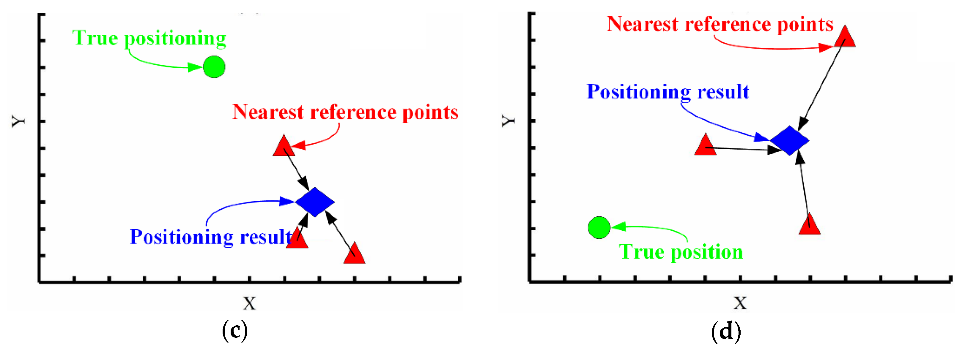
4.3. Description of TD

TD was defined as the fusion of three signal-domain distances, and it was the sum of three normalized signal-domain distances, which can be expressed as:
T D = N o r ( E D ) + N o r ( M D ) + N o r ( C D ) = [ E D 1 N o r + M D 1 N o r + C D 1 N o r   E D 2 N o r + M D 2 N o r + C D 2 N o r   E D 3 N o r + M D 3 N o r + C D 3 N o r E D 3 N o r + M D 3 N o r + C D 3 N o r ] ,
where T D denotes the sum of three normalized signal-domain distances, and E D , M D , and C D represent the signal-domain distances based on ED, MD, and CD, respectively, and E D i N o r , E D i N o r , and E D i N o r represent the normalized values of ED, MD, CD between the online fingerprint and the i t h offline fingerprint.

4.4. DBSCAN and TD Integrated WKNN Algorithm

In order to enhance the performance of fingerprinting, this paper proposed the DBSCAN and TD integrated WKNN algorithm, which applied TD to enhance the probability of obtaining reliable RPs, and adaptively selected an optimal signal-domain distance to achieve the positioning computation, and used the proposed rule to judge whether RPs were credible. There were two stages in the proposed algorithm: offline and online stages. In the offline stage, the RSS measurements on existing RPs were collected with the smartphone. Then, the mean of a sequence of RSS and coordinates of RPs were utilized to build the fingerprint database. The online stage included three steps: same RPs judgment, clustering and distance selection, and positioning calculation.
Initially, the offline fingerprints were gathered, as shown below:
RSS = { r s s 1 , r s s 2 ,   r s s N } .
Based on the signal-domain distance computation method, ED, MD, and CD between the offline fingerprints and fingerprint databases were calculated. Then, the normalization algorithm with an interval of 1 to 10 (P in Equation (6) is 10, the slope k is 9) was used to adjust the ED, MD, and CD to the same metric, which can be expressed as:
[ N o r ( E D ) N o r ( M D ) N o r ( C D ) ] = [ d i s t 1 E _ N , d i s t 2 E _ N ,   d i s t M E _ N d i s t 1 M _ N , d i s t 2 M _ N ,   d i s t M M _ N d i s t 1 C _ N , d i s t 2 C _ N ,   d i s t M C _ N ] .
We could obtain K nearest RPs according to single normalized signal-domain distance, as shown in Equation (16). In Equation (17), the nearest RP found by each signal-domain distance was available and the RP corresponding to the minimum distance was credible. Finally, these credible RPs were used to obtain the positioning results, and WKNN was employed as the positioning algorithm.
[ RP E D RP M D RP C D ] = [ { ( x 1 E D , y 1 E D ) , ( x 2 E D , y 2 E D ) , , ( x K E D , y K E D ) } { ( x 1 M D , y 1 M D ) , ( x 2 M D , y 2 M D ) , , ( x K M D , y K M D ) } { ( x 1 C D , y 1 C D ) , ( x 2 C D , y 2 C D ) , , ( x K C D , y K C D ) } ]
RP E D = RP M D = RP C D
However, the nearest RPs searched by ED, MD and CD are often different, indicating that there may be unreliable RPs. Thus, we should choose the optimal distance to perform positioning to reduce the probability of getting unreliable RPs. That is, one, two, or three distances can be used in each localization process to realize high-precision fingerprinting according to the actual situation.
In this paper, we used the number of clusters as the index of distinction degree of signal-domain distance. A greater number of clusters indicated more resolution. DBSCAN and fused distance were used for clustering of RPs, and there were three fused distances, which can be denoted as:
[ D i s t E _ P D i s t M _ P D i s t C _ P ] = [ ( d i s t 1 E _ P , d i s t 2 E _ P ,   , d i s t K E _ P ) ( d i s t 1 M _ P , d i s t 2 M _ P ,   , d i s t K M _ P ) ( d i s t 1 C _ P , d i s t 2 C _ P ,   , d i s t K C _ P ) ] .
where d i s t i E _ P is the fused distance of the i t h signal-domain ED and position-domain distance, and d i s t i M _ P presents the fused distance of the i t h signal-domain MD and position-domain distance, and d i s t i C _ P presents the fused distance of the i t h signal-domain CD and position-domain distance.
Based on these fused distances, we could obtain three groups of clustering results, as shown below:
[ C l u s t e r E _ P C l u s t e r M _ P C l u s t e r C _ P ] = [ ( c l u s t e r 1 E _ P , c l u s t e r 2 E _ P ,   , c l u s t e r l 1 E _ P ) ( c l u s t e r 1 M _ P , c l u s t e r 2 M _ P ,   , c l u s t e r l 2 M _ P ) ( c l u s t e r 1 C _ P , c l u s t e r 2 C _ P ,   , c l u s t e r l 3 C _ P ) ] .
where C l u s t e r E _ P , C l u s t e r M _ P , and C l u s t e r M _ P represent the cluster sets based on three fused distances, respectively, and c l u s t e r i E _ P present the i t h cluster in C l u s t e r E _ P , and l 1 , l 2 , and l 3 are the number of clusters. Theoretically, the larger the number of clusters is, the higher resolution of distance used for clustering is. This rule can be utilized to select the optimal signal-domain distance and improve the positioning accuracy.
We designed an adaptive selection strategy of the optimal signal-domain distance and reliable RPs according to three cases of l 1 , l 2 , and l 3 , as shown below.
Case 1: l 1 = l 2 = l 3 .
In this situation, the degree of differentiation between ED, MD, and CD was considered to be consistent. TD (ED, MD, and CD) were simultaneously applied to calculate the positioning results, as shown in Equation (20).
D i s t o p t i m a l = T D = N o r ( E D ) + N o r ( M D ) + N o r ( C D )
Then, we sorted the D i s t o p t i m a l and found the nearest RPs of density threshold quantity. The coordinates and signal-domain distance of these nearest RPs were utilized to estimate the location. WKNN algorithm was used as the positioning algorithm.
Case 2: l i > l j = l k   | | l i < l j = l k   , ( i j k , i , j , k = 1 , 2 , 3 ) .
There were two situations under this case. One was that there was two maximum number of clusters, and the other was that there was a maximum number of clusters. We chose the signal-domain distance corresponding to the maximum number of clusters, as shown below.
D i s t o p t i m a l = [ N o r ( E D ) + N o r ( M D )   ( l 1 = l 2 > l 3 ) N o r ( E D )   ( l 1 > l 2 = l 3 ) N o r ( M D ) + N o r ( C D ) ( l 2 = l 3 > l 1 )   N o r ( M D ) ( l 2 > l 1 = l 3 ) N o r ( E D ) + N o r ( C D ) ( l 2 = l 3 > l 1 ) N o r ( C D ) ( l 3 > l 1 = l 2 ) ]
Then, we sorted the D i s t o p t i m a l and found the nearest RPs. The coordinates and signal-domain distance of these nearest RPs were utilized to estimate the location. WKNN algorithm was applied for positioning, and K value was M i n p t s , i.e., density threshold.
Case 3: l i > l j > l k   , ( i j k , i , j , k = 1 , 2 , 3 ) .
There was a maximum number of clusters. We selected the signal-domain distance corresponding to the maximum number of clusters, as shown below.
D i s t o p t i m a l = [ N o r ( E D )   ( l 1 = max ( l 1 , l 2 , l 3 ) ) N o r ( M D )   ( l 2 = max ( l 1 , l 2 , l 3 ) ) N o r ( C D )   ( l 3 = max ( l 1 , l 2 , l 3 ) ) ]
Then, the nearest RPs could be found and used to estimate the location. WKNN with K value of M i n p t s was the positioning algorithm.
In this paper, the parameter α of the fused distance was 0.7, and the value of M i n P t s was 3, and the neighborhood radius E p s was 3.1 m, because the position-domain distance accounted for 30% of the fusion distance. The above parameters will remain changeless in the following tests to prove the universality of the proposed algorithm.

5. Experiment

All positioning algorithms were achieved based on the MATLAB 2021b simulation platform. SVM, GPR, and rank algorithms were selected as the comparison methods to assess the positioning performance of the proposed algorithm. Mean absolute error (MAE) and root mean square error (RMSE) were used as the indexes of accuracy and stability, respectively. MAE is the arithmetic average of the absolute errors between estimated values and true values. RMSE is the square root of the quadratic mean of differences between estimated values and true values.
Offline fingerprints and their corresponding coordinates were utilized as the training data to construct positioning models for SVM, GPR, and rank algorithms. A Bayesian optimization algorithm was employed to solve the parameters of SVM. The parameters of GPR model were solved with the quasi-Newton algorithm. Rank algorithm applied the sorting results of RSS measurements to achieve the position calculation.

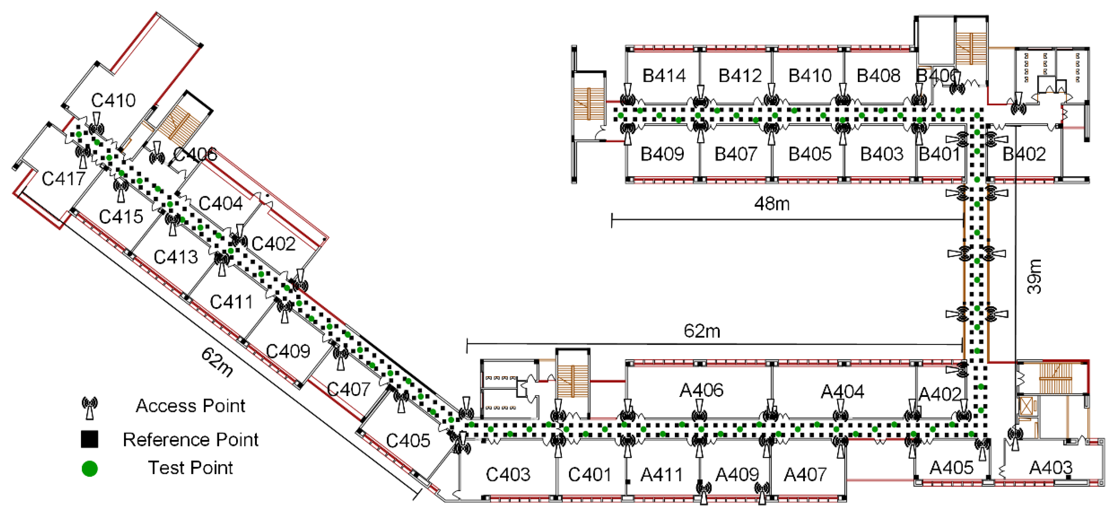
5.1. Experiment Area and Experimental Description

There were two classic scenarios for experimental tests, Scenarios A and B, as shown in Figure 4 and Figure 5.
Scenario A was a large room, the graduate student’s laboratory, with a complex layout, and easily seen in the existing indoor environment. The maximum length and width were 19.43 m and 18 m, respectively. In this scenario, there were 67 RPs marked by orange circles and 24 TPs marked by blue circles. The interval of most RPs was 1.2 m, while that of some RPs was 1.8 m. Both the existing layout and the tiles with the length and width of 60 cm determined the interval, facilitating the establishment of indoor grids. TPs were arranged randomly, and the 24th TP was outside the indoor grid. Eight APs using a Wi-Fi 6th generation protocol with a dual frequency band were pre-placed in different heights in the large room. Six APs were fixed on the wall at a height of 4 m, and one AP was placed at a height of 2 m on a steel filing cabinet, which was marked by the letter F. These seven APs were on the left of the large room. The another one was set on a big wooden table on the right of the room. Besides, another 17 APs were outside the room and arranged at different locations, such as in the long corridor, meeting room, and office room. The collection time and frequency of each RP were 80 s and 1Hz, respectively, and those at each TP were 40 s and 1 Hz, respectively. During RSS collection, all personnel in this room and somewhere else were moving normally. Many MAC addresses could be heard at each RP and TP. The lost RSS was replaced by −100 dBm.
Scenario B was a corridor with an overall length of 211 m and had almost 3200 m2. The black solid squares and green solid circles represent RP and TP, respectively. The distance between two adjacent RPs was 1.2 m and the total number of RPs was 379. The RSS data were collected on every RP and used to generate the fingerprints. The sampling time was 60 s and the sampling frequency was 1 Hz.
The test data should be collected to evaluate the performance of the proposed algorithm after the RSS data collection on RPs was completed. The total number of TPs was 86. The acquisition time and frequency were 10 s and 1 Hz, respectively. The data of 10 s was taken as one set of test data.

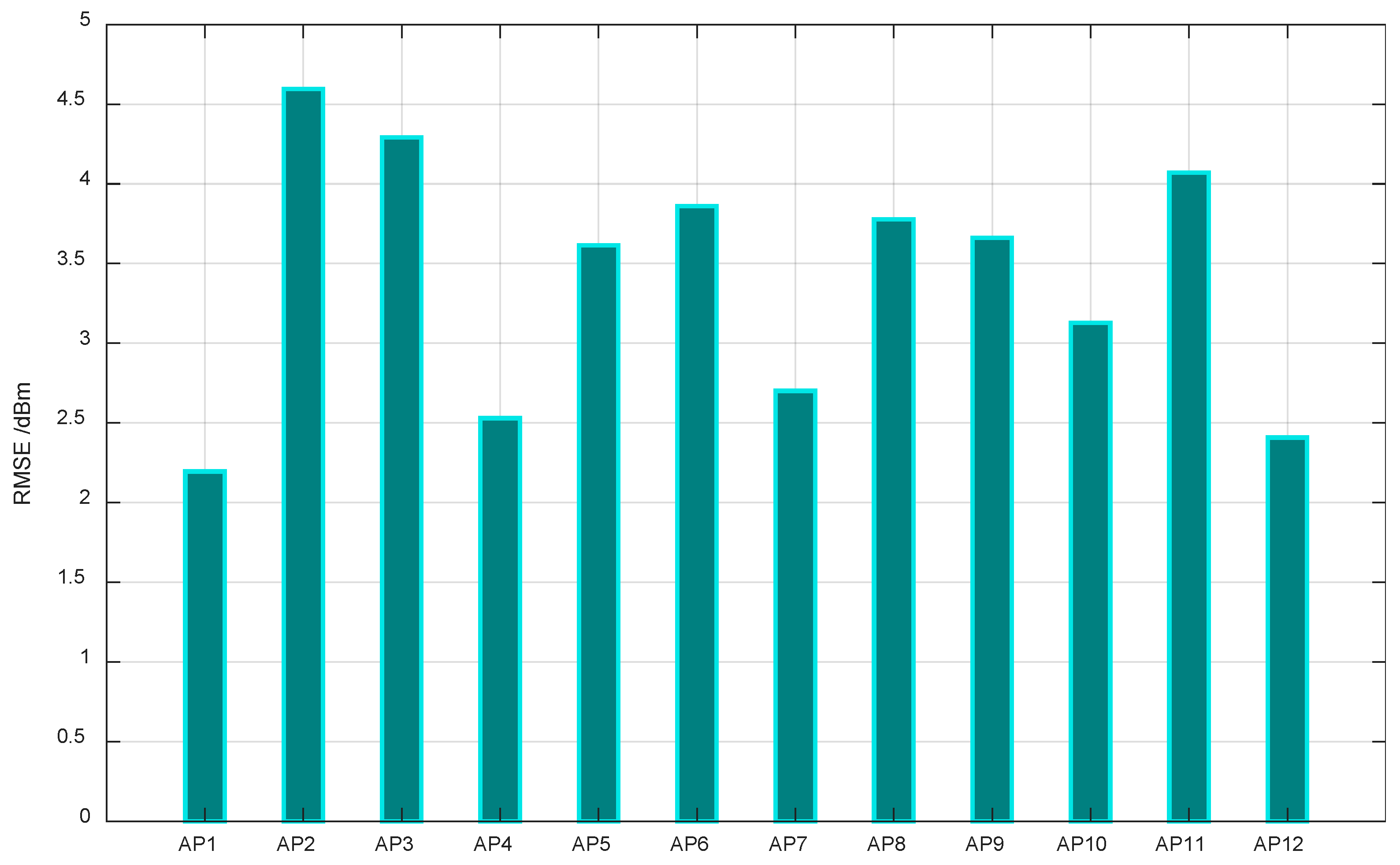
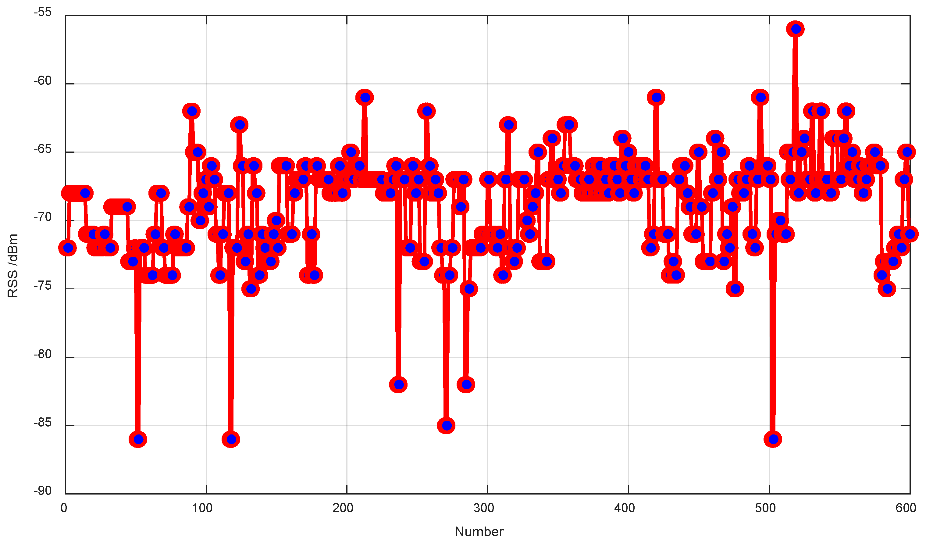
5.2. Stability of RSS Measurement

This subsection will mainly study the stability of RSS measurements by applying RMSE of ten minutes RSS measurements at a fixed location. The approximate true value of RSS was hard to acquire due to the complexity of radio propagation and the lack of high-precision measuring equipment. Thus, the accuracy analysis of RSS measurements was hard to conduct. While the mean of RSS measurements for a long time could be seen as true value. Based on the mean of RSS measurements, RMSE of RSS measurements might be obtained and regarded as an index of stability of RSS measurements.
Figure 6 presented the RMSEs of 600 groups of RSS measurements from 12 APs. All RMSEs are greater than 2 dBm, which indicated that there were wide fluctuations in the RSS measurements. In order to analyze the change of the RSS measurements, the RSS measurement of AP 6 was selected as experimental data, as shown in Figure 7. The difference between the maximum and minimum RSS measurements was 30 dBm, which could cause a large positioning error. When facing the above huge changes, the acquired nearest RPs of each positioning request might be different even if at the same position, which caused the changes of multiple localization results of the same position. Thus, it is necessary to select an optimal signal-domain distance to reduce the impact of RSS fluctuations in terms of positioning accuracy and stability.

5.3. Impact of the Number of APs and RPs on Positioning Accuracy

In this subsection, we firstly studied the impact of the number of APs on positioning accuracy. The number of deployed APs in the scenario was 8. The number of corresponding MAC addresses was 16. Because there were 17 APs displayed outside the scenario A, 50 MAC addresses could be detected in total at RP and TP. Therefore, 16 and 50 MAC addresses were used for estimating position, respectively, and WKNN was the localization algorithm. Figure 8 gives the MAEs of WKNN positioning method with 16 and 50 MAC addresses under different K values from 1 to 10. The MAE of WKNN positioning method with 50 MAC addresses was smaller than that with 16 APs on any K value. However, with the increase of K value, the difference of MAE between positioning method with 50 and 16 MAC addresses under the same K value was getting smaller gradually. At some large K value, the difference may become very small—close to zero. When K was between 1 and 10, the more the number of APs was, the higher the positioning accuracy was.
Then, the influence of the number of RPs on positioning accuracy was studied. The test area was Scenario B, and the number of RPs used in fingerprinting localization were 352, 126, 62 and 36. NN was the positioning algorithm. The experimental results were shown in Table 2. We could find a trend that the accuracy would become better with the increasing number of RPs.

5.4. Differences among ED, MD, and CD

The experiment was conducted to study the positioning effect under different signal-domain distances, and the test area was Scenario B. The ED-based signal-domain distances, MD-based signal-domain distances and CD-based signal-domain distances were calculated with the online fingerprint and fingerprint database, respectively, and the nearest RPs were found based on different signal-domain distances, respectively. Then, the positioning results were obtained with the NN algorithm.
The positioning errors of WKNN based on ED, MD, and CD, respectively, are shown in Figure 9. The positioning results varied when the signal-domain distance was different. To show the positioning effects based on different signal-domain distances, two small areas including multiple points were chosen to show the positioning performance, as illustrated in Figure 9a,b. In Figure 9a, the ED-based signal-domain distance was best at Point 22, while in Figure 9b, the CD-based signal-domain distance might be best at Point 46. And Figure 9b presented that the optimal signal-domain distance was MD at Point 47. The experimental results showed that the positioning results were different when the signal-domain distance was different. However, when three signal-domain distances were simultaneously used for positioning estimation, more reliable nearest RPs could be acquired. Thus, this paper proposed the WKNN algorithm based on TD, aiming to get more reliable nearest RPs.

5.5. Positioning Performance by Using TD

TD aims to increase the possibility of getting reliable nearest RPs and improve positioning precision. The experiment was conducted to research the positioning effect of TD, and NN was the positioning algorithm. TD was compared with ED, MD, and CD. The experimental results were shown in Figure 10. It could be seen that the positioning effect of TD was better than those of ED, MD, and CD.
The positioning effect of TD was the best among the four algorithms, with an MAE of 2.784 m and a standard deviation (STD) of 2.472 m. The MEs of MD, CD, ED were 3.092 m, 2.796 m, and 3.038 m, respectively. Besides, the RMSE of TD was lower than those of MD, CD, and ED.
Besides, the results indicated that the use of TD could improve the positioning effect and apply the advantages of three signal-domain distances. However, the TD-based fingerprinting could not select the optimal signal-domain distance for each localization, which might be the reason that the MAE of TD was similar to MD. Therefore, the realization of high-precision positioning needs to select optimal signal-domain distances.

5.6. Clustering Effect of DBSCAN

In this subsection, we will introduce the clustering effect of DBSCAN. Figure 11 shows the clustering effect of three positioning methods. In this paper, the value of M i n P t s was three.
Fused distances based on ED, MD, and CD were the fusion of position-domain distance and one of three signal-domain distances, ED-based signal-domain distance, MD-based signal-domain distance and CD-based signal-domain distance, respectively. The clustering results showed that DBSCAN using the fused distance had good clustering effects. The number of clusters was different when fused distances were different. This denoted the distinction degree of the fused distance was different in once localization.
In Figure 11a, the number of clusters based on three fused distances, respectively, was the same. The clustering results of fused distances based on CD, MD, and ED were similar. This indicated that there was a small difference among the three fused distances. In Figure 11b,c, the bigger the distinction degree of the fused distance was, the more the number of clusters was.

5.7. Performance of the Proposed DBSCAN-TD Integration WKNN Algorithm in Scenario A

In this subsection, we will evaluate the proposed method in Scenario A. Based on the collected testing data, the positioning experiment was conducted to study the stability and accuracy of the proposed method. The MAE was regarded as the index of accuracy. The stability of the positioning algorithm was measured with the RMSE. In order to rate the performance of the proposed algorithm, SVM, GPR, and rank were used as comparison algorithms.
The experimental results are shown in Figure 12. The MAE and RMSE of the pro-posed algorithm were 3.721 and 4.227 m, respectively, and those of SVM were 5.077 and 5.734 m, respectively. The MAEs of GPR and rank were 4.313 and 4.979 m, respectively, and RMSEs of those were 4.835 and 5.607 m, respectively. Note that the K of rank was 21.
More detailed errors are shown in Table 3. Compared with SVM, the stability and accuracy of the proposed algorithm were improved by 26.71% and 26.29%. The positioning precision of the proposed algorithm was improved by 13.72% and 25.26%, respectively, compared with GPR and rank. The stability of the proposed algorithm had an improvement of 12.58% and 24.61%, respectively, compared with GPR and rank.
Besides, the maximum errors of SVM, GPR, rank and proposed algorithm were 9.562, 8.729, 9.737, and 8.256 m. The maximum error of the proposed algorithm was lower than those of SVM, GPR, and rank. Therefore, the proposed algorithm was better than SVM, GPR, and rank, which is more suitable in a room with a complex layout for positioning.
Actually, the positioning performances of SVM, GPR, rank and the proposed algorithm were not ideal in Scenario A, and the minimum MAE was only 3.721 m. Based on the description of Section 5.1, the number of APs in Scenario A was enough for relatively high fingerprint localization in theory. However, the actual positioning effect was not very good. The reason should be that the Wi-Fi signals were seriously disturbed by the complex layout of Scenario A, pedestrians, etc. The proposed algorithm still had great improvement, compared with SVM, GPR, and rank, indicating that the proposed algorithm could perform better in a complex scenario.

5.8. Performance of the Proposed DBSCAN-TD Integration WKNN Algorithm in Scenario B

This subsection will mainly illustrate the performance of the proposed algorithm in Scenario B. SVM, GPR, and rank were also utilized as comparison algorithms. The experimental results are shown in Figure 13, which were the cumulative distribution functions (CDFs) of the SVM, GPR, rank, and proposed algorithm. The maximum errors were 16.696, 19.992, 22.615, and 8.461 m, respectively. This indicated that the proposed method could avoid large errors and had better stability. In addition, the minimum errors were 0.138, 0.444, 0.209, and 0.014 m, proving that the proposed algorithm had decimeter-level positioning ability.
Besides, the experimental area was a relatively huge opening-working area, so many external factors, such as multipath, non-line of sight, pedestrians, may influence the accuracy of fingerprinting. Generally, the fingerprint positioning in a larger indoor environment has poor performance. However, the probability of positioning error of the proposed method lower than 1 m reached 33.7%, and those probabilities of SVM, GPR, and rank were 10.47%, 12.79%, and 12.79%, respectively. Obviously, the proposed method achieved a bigger probability that made positioning errors below 1 m.
Figure 14 shows the positioning effects of SVM, GPR, rank, and the proposed method. The upper quartile, median, and lower quartile of the proposed method were better than those of SVM, GPR and rank. Therefore, the positioning effects of the pro-posed method was better than those of SVM, GPR, and rank.
Table 4 shows the detailed statistical results of positioning errors of SVM, GPR, rank and proposed method. The cumulative error probabilities (50%, 70% and 90%) and corresponding errors are shown for comprehensive comparison. For example, the 50% errors of SVM, GPR, rank, and the proposed method were 3.215, 3.127, 4.515, and 1.745 m, which indicated that the proposed algorithm owned a better performance.
Besides, the MAEs and RMSEs of SVM, GPR, rank and the proposed method were also displayed in Table 4. The MAE and RMSE of the proposed method were 2.094 and 2.638 m, respectively. The MAEs of SVM, GPR and rank were 3.82, 3.63, and 5.293 m, respectively, and the RMSEs of SVM, GPR, and rank were 4.735, 4.583, and 6.753 m, respectively. Obviously, rank had the worst positioning effect, with a poor accuracy and stability.
Compared with SVM, GPR, and rank, the MAE of the proposed method was reduced by 45.18, 42.31, and 60.44%, respectively. The RMSE of the proposed method had a great improvement of 44.29, 42.44, and 60.94%, respectively. This indicated that SVM, GPR, and rank were not suitable for a large indoor environment, compared with the proposed method.
Therefore, the positioning performance of the proposed method was better than that of SVM, GPR, and rank in both complex and large indoor environments.

6. Conclusions

This paper proposed a novel DBSCAN and three distances (TD) integrated Wi-Fi positioning algorithm. Three distances, DBSCAN, and high-resolution distance selection principle were combined to obtain more reliable adjacent RPs and optimal signal-domain distance in the online stage with the improvement of positioning performance. And the fused distance was enhanced by a normalization algorithm with changeable intervals, which could not only consider both the spatial layout and signal strength of RPs, but also map position-domain and signal-domain distances into the same metrics. Since the proposed method needs a period of observation time, while the speed of a walking person or moving object is larger than 1 m/s. So, our proposed method is applicable only for the location of devices or objects in semi-stationary conditions.
Scenario A is a complex-layout room with many post-graduates and a complex layout, and Scenario B is a large indoor environment covering 3200 m2. Scenarios A and B are typical representatives of large and complex indoor environment. Compared with SVM, GPR and rank positioning methods, the improvement rates of positioning accuracy and stability of the proposed algorithm in Scenarios A and B were up to 60.44% and 60.93%, respectively. Therefore, the proposed algorithm has a better positioning performance in large and complex indoor environment.

Author Contributions

Conceptualization, H.C., J.B. and K.L.; data curation, J.B., H.C. and M.Z.; formal analysis, H.C. and J.B.; funding acquisition, Y.W. and J.B.; methodology, J.B.; project administration, Y.W.; software, J.B. and G.Z.; supervision, Y.W.; validation, J.B. and N.C.; visualization, H.C.; writing—original draft, H.C. and J.B. All authors have read and agreed to the published version of the manuscript.

Funding

This research was funded by the National Natural Science Foundation of China, grant number 42001397; the National Key Research and Development Program of China, grant number 2016YFB0502102; the State Key Laboratory of Satellite Navigation System and Equipment Technology, grant number CEPNT-2018KF-03; the Introduction and Training Program of Young Creative Talents of Shandong Province, grant number 0031802; the Doctoral Research Fund of Shandong Jianzhu University, grant number XNBS1985; the Key Laboratory of Surveying and Mapping Science, and the Geo-spatial Information Technology of Ministry of Natural Resources, grant number 2020-3-4; the State Key Laboratory of Geo-Information Engineering, grant number SKLGIE2020-M-1-1.

Acknowledgments

The authors thank the editors and reviewers of this paper for their comments with which its quality was improved.

Conflicts of Interest

The authors and their institutions declare no conflict of interest.

References

  1. He, Z.; Petovello, M.G.; Pei, L.; Olesen, D.H. Evaluation of GPS/BDS indoor positioning performance and enhancement. Adv. Space Res. 2017, 59, 870–876. [Google Scholar] [CrossRef] [Green Version]
  2. Ardiansyah, A.; Nugraha, G.D.; Han, H.; Deokjai, C.; Kim, J. A decision tree-based NLOS detection method for the UWB indoor location tracking accuracy improvement. Int. J. Commun. Syst. 2019, 32, e3997. [Google Scholar]
  3. Poulose, A.; Han, D.S. UWB indoor localization using deep learning LSTM networks. Appl. Sci. 2020, 10, 6290. [Google Scholar] [CrossRef]
  4. Li, B.; Zhao, K.; Sandoval, E.B. A UWB-Based Indoor Positioning System Employing Neural Networks. J. Geovis. Spat. Anal. 2020, 4, 18. [Google Scholar] [CrossRef]
  5. Chen, L.; Pei, L.; Kuusniemi, H.; Chen, Y.; Kroger, T.; Chen, R. Bayesian Fusion for Indoor Positioning Using Bluetooth Fingerprints. Wirel. Pers. Commun. 2013, 70, 1735–1745. [Google Scholar] [CrossRef]
  6. Zhou, C.; Yuan, J.; Liu, H.; Qiu, J. Bluetooth Indoor Positioning Based on RSSI and Kalman Filter. Wirel. Pers. Commun. 2017, 96, 4115–4130. [Google Scholar] [CrossRef]
  7. Poulose, A.; Kim, J.; Han, D.S. A sensor fusion framework for indoor localization using smartphone sensors and Wi-Fi RSSI measurements. Appl. Sci. 2019, 9, 4379. [Google Scholar] [CrossRef] [Green Version]
  8. Beomju, S.; Jung Ho, L.; Taikjin, L.; Hyung Seok, K. Enhanced Weighted K-Nearest Neighbor Algorithm for Indoor WI-FI Positioning Systems. In Proceedings of the 8th International Conference on Computing Technology and Information Management (NCM and ICNIT), Seoul, Korea, 24–26 April 2012; Volume 2, pp. 574–577. [Google Scholar]
  9. Xie, Y.; Wang, Y.; Nallanathan, A.; Wang, L. An Improved K-Nearest-Neighbor Indoor Localization Method Based on Spearman Distance. IEEE Signal Process. Lett. 2016, 23, 351–355. [Google Scholar] [CrossRef] [Green Version]
  10. Zhang, D.; Yang, L.T.; Min, C.; Zhao, S.; Guo, M.; Yin, Z. Real-Time Locating Systems Using Active RFID for Internet of Things. IEEE Syst. J. 2017, 10, 1226–1235. [Google Scholar] [CrossRef]
  11. Yao, C.; Hsia, W. An Indoor Positioning System Based on the Dual-Channel Passive RFID Technology. IEEE Sens. J. 2018, 18, 4654–4663. [Google Scholar] [CrossRef]
  12. Zhuang, X.; Yu, X.; Zhou, D.; Zhao, Z.; Zhang, W.; Li, L.; Liu, Z. A novel 3D position measurement and structure prediction method for RFID tag group based on deep belief network. Measurement 2019, 136, 25–35. [Google Scholar] [CrossRef]
  13. Liu, Z.; Chen, R.; Ye, F.; Guo, G.; Li, Z.; Qian, L. Improved TOA Estimation Method for Acoustic Ranging in a Reverberant Environment. IEEE Sens. J. 2020, 1–8. [Google Scholar] [CrossRef]
  14. Khyam, M.O.; Rahim, M.N.A.; Li, X.; Jayasuriyaet, A.; Mahmud, M.A.; Oo, A.M.T. Simultaneous excitation systems for ultrasonic indoor positioning. IEEE Sens. J. 2020, 20, 13716–13725. [Google Scholar] [CrossRef]
  15. Ma, Y.; Dou, Z.; Jiang, Q.; Hou, Z. Basmag: An Optimized HMM-Based Localization System Using Backward Sequences Matching Algorithm Exploiting Geomagnetic Information. IEEE Sens. J. 2016, 16, 7472–7482. [Google Scholar] [CrossRef]
  16. Gao, Y. An Improved Particle Filter Algorithm for Geomagnetic Indoor Positioning. J. Sens. 2018, 2018, 5989678. [Google Scholar]
  17. Fujii, K.; Yonezawa, R.; Sakamoto, Y.; Schmitz, A.; Sugano, S. A Combined Approach of Doppler and Carrier-Based Hyperbolic Positioning with a Multi-Channel GPS-Pseudolite for Indoor Localization of Robots. In Proceedings of the International Conference on Indoor Positioning and Indoor Navigation (IPIN), Madrid, Spain, 4–7 October 2016; pp. 1–7. [Google Scholar]
  18. Li, X.; Zhang, P.; Huang, G.; Zhang, Q.; Zhao, Q. Performance analysis of indoor pseudolite positioning based on the unscented Kalman filter. GPS Solut. 2019, 23, 79. [Google Scholar] [CrossRef]
  19. Xiao, A.; Ruizhi, C.; Deren, L.; Yujin, C.; Dewen, W. An Indoor Positioning System Based on Static Objects in Large Indoor Scenes by Using Smartphone Cameras. Sensors 2018, 18, 2229. [Google Scholar] [CrossRef] [Green Version]
  20. Yao, G.; Yilmaz, A.; Zhang, L.; Meng, F.; Ai, H.; Jin, F. Matching Large Baseline Oblique Stereo Images Using an End-To-End Convolutional Neural Network. Remote Sens. 2021, 13, 274. [Google Scholar] [CrossRef]
  21. Zhang, Y.; Tan, X.; Zhao, C. UWB/INS integrated pedestrian positioning for robust indoor environments. IEEE Sens. J. 2020, 20, 14401–14409. [Google Scholar] [CrossRef]
  22. Poulose, A.; Eyobu, O.S.; Han, D.S. An indoor position-estimation algorithm using smartphone IMU sensor data. IEEE Access 2019, 7, 11165–11177. [Google Scholar] [CrossRef]
  23. Poulose, A.; Han, D.S. Hybrid Indoor Localization Using IMU Sensors and Smartphone Camera. Sensors 2019, 19, 5084. [Google Scholar] [CrossRef] [Green Version]
  24. Sun, M.; Wang, Y.; Xu, S.; Qi, H.; Hu, X. Indoor positioning tightly coupled Wi-Fi FTM ranging and PDR based on the extended Kalman filter for smartphones. IEEE Access 2020, 8, 49671–49684. [Google Scholar] [CrossRef]
  25. Li, C.; Zhen, J.; Chang, K.; Xu, A.; Zhu, H.; Wu, J. An Indoor Positioning and Tracking Algorithm Based on Angle-of-Arrival Using a Dual-Channel Array Antenna. Remote Sens. 2021, 13, 4301. [Google Scholar] [CrossRef]
  26. Poulose, A.; Han, D.S. Performance Analysis of Fingerprint Matching Algorithms for Indoor Localization. In Proceedings of the International Conference on Artificial Intelligence in Information and Communication (ICAIIC), Fukuoka, Japan, 19–21 February 2020; pp. 661–665. [Google Scholar]
  27. Liu, F.; Liu, J.; Yin, Y.; Wang, W.; Hu, D.; Chen, P.; Niu, Q. Survey on WiFi-based indoor positioning techniques. IET Commun. 2020, 14, 1372–1383. [Google Scholar] [CrossRef]
  28. Feng, X.; Nguyen, K.A.; Luo, Z. A survey of deep learning approaches for WiFi-based indoor positioning. J. Inf. Telecommun. 2021, 1–54. [Google Scholar] [CrossRef]
  29. Mendoza-Silva, G.M.; Torres-Sospedra, J.; Huerta, J. A meta-review of indoor positioning systems. Sensors 2019, 19, 4507. [Google Scholar] [CrossRef] [PubMed] [Green Version]
  30. Bahl, P.; Padmanabhan, V.N. RADAR: An In-Building RF-Based User Location and Tracking System. In Proceedings of the IEEE INFOCOM, Tel Aviv, Israel, 6 August 2000; Volume 2, pp. 775–784. [Google Scholar]
  31. Oh, J.; Kim, J. Adaptive K-nearest neighbour algorithm for WiFi fingerprint positioning. ICT Express 2018, 4, 91–94. [Google Scholar] [CrossRef]
  32. Xie, H.; Gu, T.; Tao, X.; Ye, H.; Lv, J. MaLoc: A Practical Magnetic Fingerprinting Approach to Indoor Localization Using Smartphones. In Proceedings of the ACM International Joint Conference on Pervasive and Ubiquitous Computing, Seattle, WA, USA, 13–17 September 2014; pp. 243–253. [Google Scholar]
  33. Tian, Z.; Tang, X.; Zhou, M.; Tan, Z. Fingerprint indoor positioning algorithm based on affinity propagation clustering. Eurasip J. Wirel. Commun. Netw. 2013, 2013, 272. [Google Scholar] [CrossRef] [Green Version]
  34. Sharp, I.; Yu, K. Enhanced Least-Squares Positioning Algorithm for Indoor Positioning. IEEE Trans. Mob. Comput. 2013, 12, 1640–1650. [Google Scholar] [CrossRef]
  35. Wu, G.; Tseng, P. A Deep Neural Network-Based Indoor Positioning Method using Channel State Information. In Proceedings of the International Conference on Computing, Networking and Communications (ICNC), Maui, HI, USA, 5–8 March 2018; pp. 290–294. [Google Scholar]
  36. Chu, C.; Yang, S. A Particle Filter Based Reference Fingerprinting Map Recalibration Method. IEEE Access 2019, 7, 111813–111827. [Google Scholar] [CrossRef]
  37. Minaev, G.; Visa, A.; Piche, R. Comprehensive survey of similarity measures for ranked based location fingerprinting algorithm. In Proceedings of the International Conference on Indoor Positioning and Indoor Navigation (IPIN), Sapporo, Japan, 18–21 September 2017; pp. 1–4. [Google Scholar]
  38. Torres-Sospedra, J.; Montoliu, R.; Trilles, S.; Belmonte, S.; Huerta, J. Comprehensive Analysis of Distance and Similarity Measures for Wi-Fi Fingerprinting Indoor Positioning Systems. Expert Syst. Appl. 2015, 42, 9263–9278. [Google Scholar] [CrossRef]
  39. Lohan, E.S.; Torres-Sospedra, J.; Leppäkoski, H.; Richter, P.; Peng, Z.; Huerta, J. Wi-Fi Crowdsourced Fingerprinting Dataset for Indoor Positioning. Data 2017, 2, 32. [Google Scholar] [CrossRef] [Green Version]
  40. Seong, J.-H.; Seo, D.-H. Wi-Fi fingerprint using radio map model based on MDLP and euclidean distance based on the Chi squared test. Wirel. Netw. 2019, 25, 3019–3027. [Google Scholar] [CrossRef]
  41. Jung, H.Y.; Yong, S.H. Fingerprint Liveness Map Construction Using Convolutional Neural Network. Electron. Lett. 2018, 54, 564–566. [Google Scholar] [CrossRef]
  42. Yiu, S.; Yang, K. Gaussian Process Assisted Fingerprinting Localization. IEEE Internet Things J. 2016, 3, 683–690. [Google Scholar] [CrossRef]
  43. Cao, H.; Wang, Y.; Bi, J.; Xu, S.; Qi, H.; Si, M.; Yao, G. WiFi RTT Indoor Positioning Method Based on Gaussian Process Regression for Harsh Environments. IEEE Access 2020, 8, 215777–215786. [Google Scholar] [CrossRef]
  44. Song, X.; Fan, X.; Xiang, C.; Ye, Q.; Liu, L.; Wang, Z.; He, X.; Yang, N.; Fang, G. A novel convolutional neural network based indoor localization framework with WiFi fingerprinting. IEEE Access 2019, 7, 110698–110709. [Google Scholar] [CrossRef]
  45. Zhang, J.; Lyu, Y.; Patton, J.; Periaswamy, S.C.G.; Roppel, T. BFVP: A Probabilistic UHF RFID Tag Localization Algorithm Using Bayesian Filter and a Variable Power RFID Model. IEEE Trans. Ind. Electron. 2018, 65, 8250–8825. [Google Scholar] [CrossRef]
  46. Li, B.; Dempster, A.G.; Barnes, J.; Rizos, C.; Li, D. Probabilistic Algorithm to Support the Fingerprinting Method for CDMA Location. In Proceedings of the International Symposium on GPS/GNSS, Hong Kong, China, 8–10 December 2005; pp. 8–10. [Google Scholar]
  47. Sangeetha, S.; Radha, N. A New Framework for IRIS and Fingerprint Recognition Using SVM Classification and Extreme Learning Machine Based on Score Level Fusion. In Proceedings of the 7th International Conference on Intelligent Systems and Control (ISCO), Coimbatore, India, 4–5 January 2013; pp. 183–188. [Google Scholar]
  48. Torres-Sospedra, J.; Moreira, A.; Knauth, S.; Berkvens, R.; Montoliu, R.; Belmonte Fernández, O.; Trilles Oliver, S.; Nicolau, M.; Meneses, F.; Costa, A.; et al. A realistic evaluation of indoor positioning systems based on Wi-Fi fingerprinting: The 2015 EvAAL–ETRI competition. J. Ambient Intell. Smart Environ. 2017, 9, 263–279. [Google Scholar] [CrossRef] [Green Version]
  49. Ali, M.U.; Hur, S.; Park, S.; Park, Y. Harvesting Indoor Positioning Accuracy by Exploring Multiple Features from Received Signal Strength Vector. IEEE Access 2019, 7, 52110–52121. [Google Scholar] [CrossRef]
  50. Sun, W.; Xue, M.; Yu, H.; Tang, H.; Lin, A. Augmentation of fingerprints for indoor WiFi localization based on Gaussian process regression. IEEE Trans. Veh. Technol. 2018, 67, 10896–10905. [Google Scholar] [CrossRef]
  51. Gowda, K.C.; Krishna, G. Agglomerative clustering using the concept of mutual nearest neighbourhood. Pattern Recognit. 1978, 10, 105–112. [Google Scholar] [CrossRef]
  52. Chen, G.; Liu, Q.; Wei, Y.; Yu, Q. An Efficient Indoor Location System in WLAN Based on Database Partition and Euclidean Distance-Weighted Pearson Correlation Coefficient. In Proceedings of the 2nd IEEE International Conference on Computer and Communications (ICCC), Chengdu, China, 14–17 October 2016; pp. 1736–1741. [Google Scholar]
  53. Retscher, G.; Joksch, J. Comparison of Different Vector Distance Measure Calculation Variants for Indoor Location Fingerprinting. In Proceedings of the 13th International Conference on Location-Based Services, Vienna, Austria, 14–16 November 2016; pp. 53–76. [Google Scholar]
  54. Pu, Y.-C.; You, P.-C. Indoor positioning system based on BLE location fingerprinting with classification approach. Appl. Math. Model. 2018, 62, 654–663. [Google Scholar] [CrossRef]
  55. Li, C.; Qiu, Z.; Liu, C. An Improved Weighted K-Nearest Neighbor Algorithm for Indoor Positioning. Wirel. Pers. Commun. 2017, 96, 2239–2251. [Google Scholar] [CrossRef]
  56. Marques, N.; Meneses, F.; Moreira, A. Combining Similarity Functions and Majority Rules for Multi-Building, Multi-Floor, WiFi Positioning. In Proceedings of the International Conference on Indoor Positioning and Indoor Navigation (IPIN), Sydney, Australia, 13–15 November 2012; pp. 1–9. [Google Scholar]
  57. Farshad, A.; Jiwei, L.; Marina, M.K.; Garcia, F.J. A Microscopic Look at WiFi Fingerprinting for Indoor Mobile Phone Localization in Diverse Environments. In Proceedings of the International Conference on Indoor Positioning and Indoor Navigation (IPIN), Montbeliard, France, 28–31 October 2013; pp. 1–10. [Google Scholar]
  58. Bi, J.; Wang, Y.; Li, X.; Cao, H.; Qi, H.; Wang, Y. A novel method of adaptive weighted K-nearest neighbor fingerprint indoor positioning considering user’s orientation. Int. J. Distrib. Sens. Netw. 2018, 14, 1550147718785885. [Google Scholar] [CrossRef]
  59. Zhou, H.; Van, N.N. Indoor Fingerprint Localization Based on Fuzzy C-Means Clustering. In Proceedings of the Sixth International Conference on Measuring Technology and Mechatronics Automation, Zhangjiajie, China, 10–11 January 2014; pp. 337–340. [Google Scholar]
  60. Ester, M.; Kriegel, H.P.; Sander, J.; Xu, X. A Density-Based Algorithm for Discovering Clusters in Large Spatial Databases with Noise. In Proceedings of the International Conference on Knowledge Discovery and Data Mining (KDD-96), Portland, OR, USA, 2–4 August 1996; Volume 14, pp. 226–231. [Google Scholar]
Figure 1. Examples of unreliable nearest RPs. (a) two nearest RPs away from true position, (b) one nearest RP away from true position, three nearest RPs away from true position in (c) and (d).
Remotesensing 14 00297 g001aRemotesensing 14 00297 g001b
Figure 2. The principle of the DBSCAN algorithm. (a) All points density-reachable from the given point p , (b) the given point p and its density-reachable points forming the cluster.
Remotesensing 14 00297 g002
Figure 3. The system overview of the proposed method.
Remotesensing 14 00297 g003
Figure 4. Scenario A. The wooden desk is in orange, the wooden cabinet is in red, the plastic chair is in blue. Wireless signal station denotes access point, reference points, and test points are illustrated in different colors.
Remotesensing 14 00297 g004
Figure 5. Scenario B. Wireless signal station denotes access point, the reference point is illustrated as a black solid square, and the test point is a green solid circle.
Remotesensing 14 00297 g005
Figure 6. RMSEs of RSS measurements from 12 APs.
Remotesensing 14 00297 g006
Figure 7. 600 groups of RSS measurements of the AP 6.
Remotesensing 14 00297 g007
Figure 8. MAEs of 16 and 50 MACs under different K values.
Remotesensing 14 00297 g008
Figure 9. Positioning errors based on ED, MD, and CD, respectively.
Remotesensing 14 00297 g009
Figure 10. Positioning errors based on ED, CD, MD, and TD, respectively.
Remotesensing 14 00297 g010
Figure 11. Clustering results of three positioning methods, (a) case 1, (b) case 2, and (c) case 3.
Remotesensing 14 00297 g011
Figure 12. MAE and RMSE of SVM, GPR, rank, and the proposed algorithm.
Remotesensing 14 00297 g012
Figure 13. CDFs of SVM, GPR, rank, and the proposed method.
Remotesensing 14 00297 g013
Figure 14. Positioning effects of SVM, GPR, rank and the proposed method.
Remotesensing 14 00297 g014
Table 1. The structure of fingerprint database.
IdLocation M A C 1 M A C 2 M A C j M A C N
1 ( x 1 , y 1 ) μ 11 μ 12 μ 1 j μ 1 N
2 ( x 2 , y 2 ) μ 21 μ 22 μ 2 j μ 2 N
i ( x i , y i ) μ i 1 μ i 2 μ i j μ i N
M ( x M , y M ) μ M 1 μ M 2 μ M j μ M N
Table 2. The MAEs of positioning method with different number of RPs.
Number of RPsMAE (m)
3523.011
1264.017
623.636
365.096
Table 3. The maximum errors, MAEs, and RMSEs of SVM, GPR, rank, and the proposed algorithm (m).
AlgorithmMaximum ErrorMAERMSE
SVM9.5625.0775.734
GPR8.7294.3134.835
Rank9.7374.9795.607
Proposed algorithm8.2563.7214.227
Table 4. Statistical results of positioning errors of SVM, GPR, rank and the proposed method (m).
Algorithm50% Error70% Error90% ErrorMAERMSE
SVM3.2154.2387.4143.8204.735
GPR3.1274.0956.3283.6304.583
Rank4.5156.20811.4075.2936.753
Proposed algorithm1.7542.6363.9702.0942.638
Publisher’s Note: MDPI stays neutral with regard to jurisdictional claims in published maps and institutional affiliations.

