Article

A Comparison of Various Correction and Blending Techniques for Creating an Improved Satellite-Gauge Rainfall Dataset over Australia

1
Bureau of Meteorology, Melbourne, VIC 3008, Australia
2
School of Mathematical and Geospatial Sciences, Royal Melbourne Institute of Technology (RMIT) University, Melbourne, VIC 3000, Australia
*
Author to whom correspondence should be addressed.
Remote Sens. 2022, 14(2), 261; https://doi.org/10.3390/rs14020261
Submission received: 4 December 2021 / Revised: 1 January 2022 / Accepted: 3 January 2022 / Published: 7 January 2022

Abstract

:
Satellites offer a way of estimating rainfall away from rain gauges which can be utilised to overcome the limitations imposed by gauge density on traditional rain gauge analyses. In this study, Australian station data along with the Japan Aerospace Exploration Agency’s (JAXA) Global Satellite Mapping of Precipitation (GSMaP) and the Bureau of Meteorology’s (BOM) Australian Gridded Climate Dataset (AGCD) rainfall analysis are combined to develop an improved satellite-gauge rainfall analysis over Australia that uses the strengths of the respective data sources. We investigated a variety of correction and blending methods with the aim of identifying the optimal blended dataset. The correction methods investigated were linear corrections to totals and anomalies, in addition to quantile-to-quantile matching. The blending methods tested used weights based on the error variance to MSWEP (Multi-Source Weighted Ensemble Product), distance to the closest gauge, and the error from a triple collocation analysis to ERA5 and Soil Moisture to Rain. A trade-off between away-from- and at-station performances was found, meaning there was a complementary nature between specific correction and blending methods. The most high-performance dataset was one corrected linearly to totals and subsequently blended to AGCD using an inverse error variance technique. This dataset demonstrated improved accuracy over its previous version, largely rectifying erroneous patches of excessive rainfall. Its modular use of individual datasets leads to potential applicability in other regions of the world.

Graphical Abstract

1. Introduction

Rainfall is a fundamental part of the water cycle that brings freshwater to Earth’s surface. The estimation of the amount of rainfall that has fallen is crucial for quantifications of water availability. This is important for many facets of society, including population health [1], disaster risk management [2], economic decisions [3], scientific modelling [4], and the protection of ecosystems [5]. Rain gauges offer a direct way of measuring rainfall that reaches the surface. Although gauges are considered the most accurate of rainfall estimates [6], they are still subject to their own biases, such as those from wind, evaporation, wetting and splashing effects, as well as those induced from the instrument and observer [7].
Another crucial limitation of rain gauges is that they offer a point-based measurement, whereas a gridded product is valuable for climate monitoring over large scales as well as for use in scientific models [8]. Point-based observations can be converted into a grid via objective analysis methods but there can be significant deficiencies where rain gauge density is low [9] and when short time scales are concerned [10]. This is because rainfall is a variable that can exhibit high spatiotemporal variation. In [11], the correlation of adjacent rain gauges in the USA was evaluated, finding that at distances of 5 km the correlation was already less than 0.5. Using this observation, in [12] it was estimated that less than 1% of the Earth’s surface could be reliably represented daily by rain gauges.
Expansion of the current rain gauge network is difficult due to both economical and physical constraints, with much of the remaining unobserved area in the world being either remote or over oceans [12]. There are also issues with how well gridded datasets can represent variability. In [13] it was found that although gridded annual totals were close to the rain gauge values, the frequency of low-precipitation events was greatly increased, while both the amount and frequency of heavy precipitation were significantly reduced. These effects are natural given that the rainfall is being spread over an area, and have implications for the representation of extreme events.
To utilise the superior performance of gauge data where spatial density is adequate [8] whilst giving more credence to non-gauge datasets in poorly observed areas, numerous corrected and blended datasets have been developed which have better performance over that of their comprising datasets, e.g., [6,14,15]. Correction refers to the calibration of a non-gauge dataset to gauge data while blending refers to the merging of a gauge dataset with one or more datasets.
However, none of these blended datasets are being used operationally in Australia. This is because existing blended datasets do not utilise a more complete set of stations that are used in the current operational dataset AGCD (Australian Gridded Climate Dataset), leading to AGCD having superior performance in well-observed areas which also correspond to areas of high population in Australia. Figure 1 (adapted from our previous study [16]) shows the typical coverage of the rain gauge network in Australia, as employed by AGCD. The exact number of stations varies due to factors such as discontinuities in operation as well as reporting time lags.
In our previous study [16], we created a blended dataset that performed well over these well-observed areas, as well as possessing a more realistic representation of rainfall over gauge-sparse regions. However, the potential for significant improvement was also identified, especially regarding the correction process used, which occasionally generated substantial positive bias.
This paper aims to develop an optimal configuration for the correction and blending of satellite data with gauge data on a monthly timescale, improving upon a previous dataset [16]. The term ‘correction’ will be used instead of ‘adjustment’ to align with convention as well as to reflect the idea that the corrected dataset is of greater quality than the original version. To achieve this, the following objectives are set:
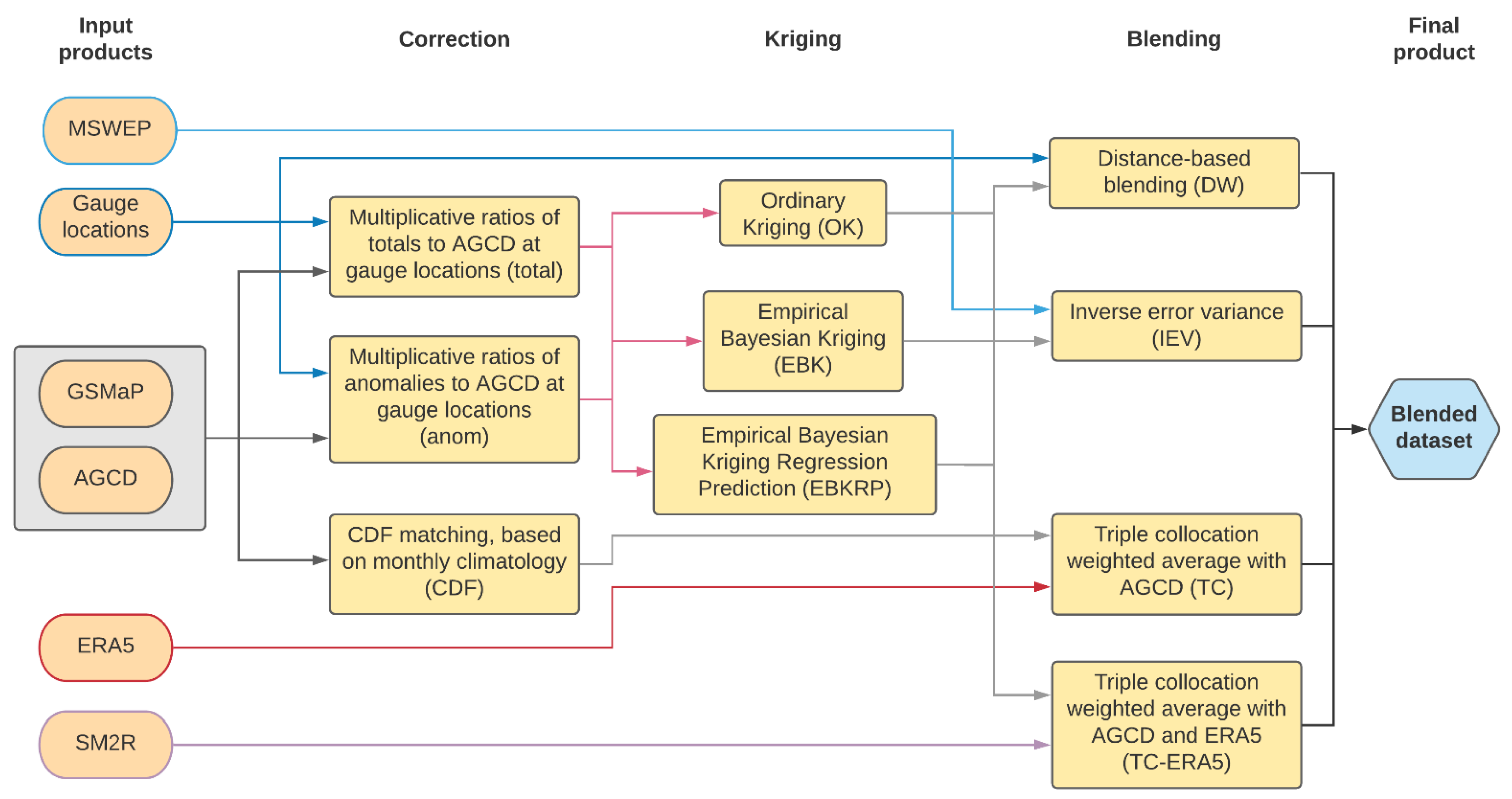
  • Several new methods of correction and blending of satellite data to gauge data will be explored. The correction techniques evaluated will be linear correction- to-totals and correction-to-anomalies methods (the former being the original technique), as well as the use of quantile-to-quantile matching. The use of Empirical Bayesian Kriging (EBK) and Empirical Bayesian Kriging Regression Prediction (EBKRP) will also be investigated to find if they offer improvements on Ordinary Kriging (OK). These corrected datasets will be blended with the gauge analysis using the original method of inverse error variance (IEV), in addition to a method that explicitly includes distance and another where the weights come from a triple collocation analysis (TCA);
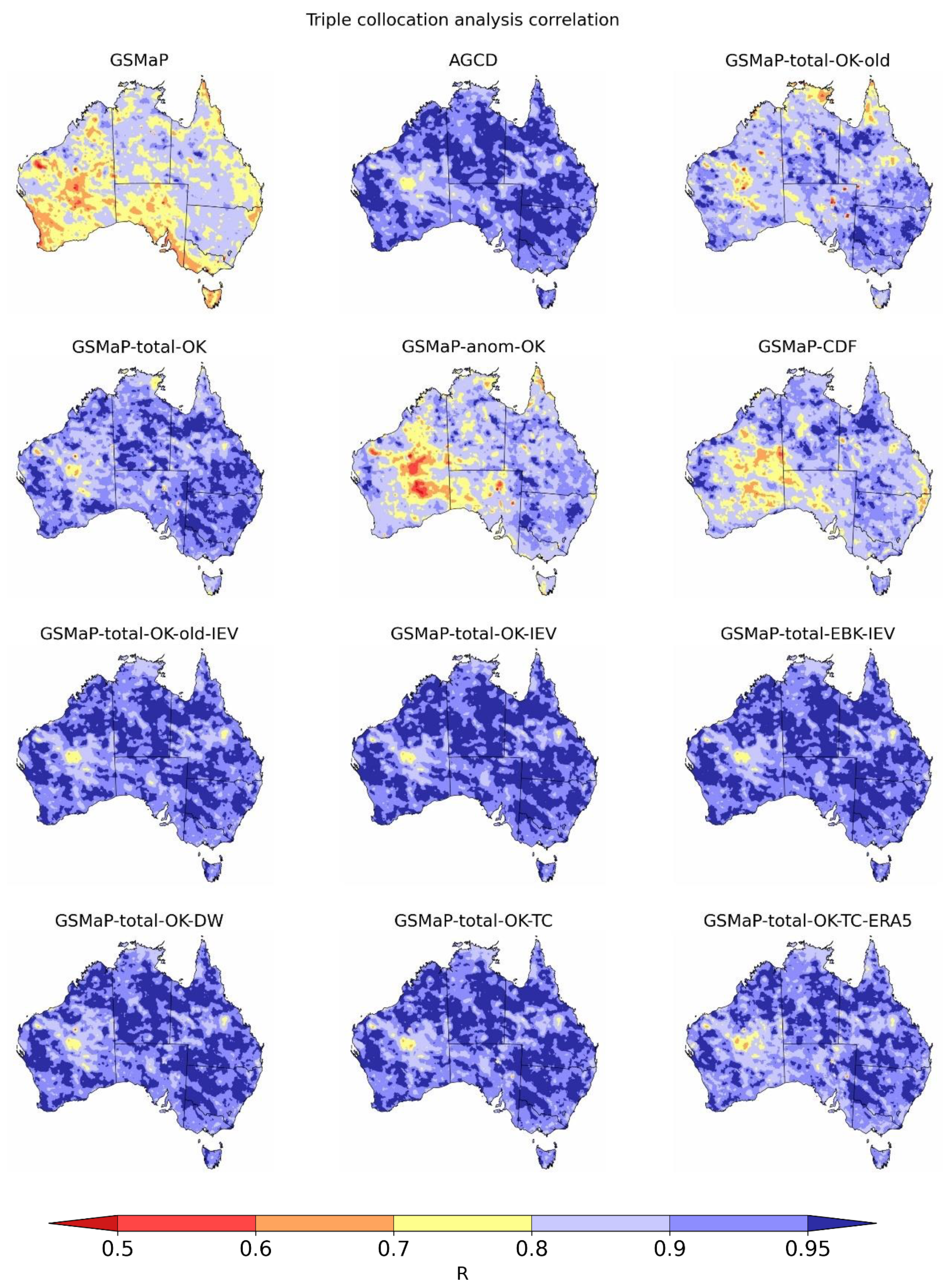
  • The efficacy of datasets built from a combination of all these techniques will be evaluated, along with an analysis of their respective advantages and disadvantages. Performance close to stations will be determined through comparison to station data, while a comparison to MSWEP along with a triple collocation analysis (TCA) will establish performance away from stations.

2. Materials and Methods

2.1. Validation

Traditional validation compares datasets against a known reference, typically one based on rain gauges. However, rain gauges (and more generally, any dataset) are subject to their own biases which conflate validation. Additionally, large parts of the world have poor coverage where the use of rain gauges as a reference would bear a great deal of uncertainty [12]. Triple collocation analysis (TCA) provides an alternative method of validation where the error [17] and correlation statistics [18] of three independent datasets (known as the triplet) can be estimated against an ‘unknown’ truth.
It was first utilised to estimate the error characteristics of wind data [17]; subsequently, it was first adapted for rainfall in [19]. Following [19], later studies (e.g., [20,21]) have demonstrated the technique is capable of providing realistic error estimates for rainfall, being especially valuable over gauge-sparse areas.
A short overview of the technique is presented below, for full details refer to [21]. The proper use of TCA relies on the key assumptions of: (1) stationarity of the data (no autocorrelation); (2) orthogonality of errors (their expected sum is zero); (3) the datasets used are linearly related; and (4) there is no correlation amongst the errors of the datasets, as well as with the truth [21].
First, the datasets in the triplets can be related to the truth using an additive model (Equation (1)):
X i = X i + ε i = α i + β i t + ε i  
where t is the truth, Xi (i = 1, 2, 3) are the triplet data which can be linearly related to the truth using the ordinary least squares intercepts αi and slopes βi, and εi are their random errors. Using one of the datasets as a reference along with the assumptions stated, the equations can be rearranged to provide an estimation of the residual errors, σε,i (Equation (2)), as well as the correlation of the datasets to the truth, ρt,Xi (Equation (3)).
σ ε , 1 = Q 11 Q 12 Q 13 Q 23 σ ε , 2 = Q 22 Q 12 Q 23 Q 13 σ ε , 3 = Q 33 Q 13 Q 23 Q 12  
ρ t , X 1 = Q 12 Q 13 Q 11 Q 23 ρ t , X 2 = s i g n ( Q 13 Q 23 ) Q 12 Q 23 Q 13 Q 22 ρ t , X 3 = s i g n ( Q 12 Q 23 ) Q 13 Q 23 Q 12 Q 33  
Qij denotes the covariances of the datasets with each other and there is a sign ambiguity for ρt,X; however, in practice, the datasets can be assumed to be positively correlated to the truth in almost all cases [18]. Intuitively, the equations depict the error for a dataset being smaller if it possesses a smaller variance and when it has strong correlations to the other datasets. The degree to which the required assumptions are satisfied by the datasets used in this study, and hence the appropriateness of this technique for this study, is explored in Appendix A. For validation, the triplet is comprised of the dataset to be verified, Soil Moisture to Rain (SM2R), and ERA5.
Three validation methods are used in this study. Performance at rain gauges was captured by validation against point station data. TCA and a gridded comparison against MSWEP (Multi-Source Weighted-Ensemble Precipitation) [6] provided additional methods of ranking the datasets, with a particular focus on performance away from rain gauges. All data were bilinearly interpolated to a resolution of 0.1 degrees (the native resolution for the blended datasets), with any negative values from the interpolation process set to zero. In the case of the point station comparison, the station value is compared to a gridded average centred at the location of the station. Consequently, a spatial representative error is expected but as it would be constant amongst the datasets, a comparison can still be made.
For the gauge and MSWEP comparisons, the mean bias (MB), root-mean-squared-error (RMSE) and Pearson correlation coefficient (R) were computed for each dataset while the TCA yielded the aforementioned error variance (σ) and correlation (ρ). These metrics were averaged over the Australian domain and a study period of 2001 to 2020.
For each verification, a dataset’s ranking was determined through ranking the mean ranking of its error and correlation statistics. This meant equal rankings could occur (such as when two datasets had the same rankings but for opposite metrics). These individual verification rankings were then averaged with the mean forming a summary statistic. This facilitated an easy-to-understand summary statistic with a focus on the relative ranking of the datasets.

2.2. Datasets

Datasets used for the development of the blended satellite datasets or its subsequent validation are described briefly below in Table 1.

2.3. Correction and Blending Methods

The performance of the existing correction and blending methods of linear correction to totals and inverse error variance weighting were evaluated against new techniques developed in this study. For detail on the existing methods, refer to [16]. In this study, there were a total of seven corrected datasets. Each corrected dataset was trialled in each blending method in case there were non-linear improvements from the blending process. The final blended datasets are created on a 0.1 × 0.1 grid to match the GSMaP data. A schematic outlining the datasets, along with their input into the various correction and blending processes, is shown in Figure 2.
The schematic also denotes the names of a dataset with a corresponding suffix being appended for each relevant process. For example, the original corrected dataset formed from a linear correction-to-totals method that was gridded using Ordinary Kriging (OK) is denoted GSMaP-total-OK. If this dataset was then blended using the original technique of IEV, the final blended dataset is denoted as GSMaP-total-OK-IEV. The ‘old’ suffix for the total-OK technique differentiates between the existing method and the refined method introduced in this study.

2.3.1. Linear Correction to Totals

The original correction technique developed was based on a linear correction-to-totals method; readers are referred to our previous study for details [16]. The presence of localised over-inflated regions of rainfall, referred to as ‘bullseyes’ hereafter, from this technique inspired some modifications. A correction to AGCD data rather than the actual point data was trialled. This reduced the mismatch in spatial sampling as the gridded values of GSMaP were corrected against corresponding gridded averages rather than to point values. At each gauge location, the value for AGCD and GSMaP was obtained through bilinear interpolation. The quotients from dividing the AGCD totals by the GSMaP totals formed a set of correction factors which was converted to a correction grid through kriging. Multiplication of GSMaP by the correction grid yielded the corrected GSMaP dataset.
Additionally, a lower threshold, for which clipping occurs if exceeded, was tested. This was to further reduce the occurrence of ‘bullseyes’, with the original threshold of ten being identified as possibly too large [16]. A variety of thresholds between two and ten were trialled, with a threshold of four providing the greatest performance. The amount of data being clipped was not significantly increased (increased from 12.3% to 15.4%), providing confidence that this new threshold was not excessively low.
A validation against MSWEP was performed to evaluate the overall performance of each of these refinements and both yielded slight improvements across all metrics. A larger reduction in RMSE compared to MAE was found, alluding to how the improvement was most significant for gross overestimations. Visual inspection also confirmed the severity of ‘bullseyes’ was considerably reduced, and although there were still occurrences, their frequency was also reduced.

2.3.2. Linear Correction to Anomalies

The value of correcting anomalies to the climatological field rather than to the actual totals was analysed. This utilised the fact that the number of stations making up the climatology field is typically much greater than those which make up the individual months, allowing spatial variability in the mean climate to be maximised [10]. Monthly anomalies tend to be driven by large-scale features and hence may be able to be sufficiently represented by a comparatively less dense network [10]. In [31] it was found that the correction to totals resulted in the problematic extrapolation of gradients over unobserved areas, leading to the generation of unrealistic extremes, an issue which was resolved by using the anomalies instead. The use of anomalies for interpolation has become a common technique and is employed in other datasets, such as the Precipitation Reconstruction (PREC) [32] and AGCD [27].
In this study, the anomaly method involved finding the ratio between the anomalies (in contrast to totals as in Section 2.3.1) of both the satellite data and the station data at each station, with respect to their own climatology. As in Section 2.3.1, this was converted into a grid through kriging, which was then applied to the original data to correct the satellite anomalies. The anomalies were then added back onto the climatology to obtain the value for each month. Clip values between ±3 and ±15 were trialled with ±8 providing the best performance.

2.3.3. Quantile to Quantile Matching

An alternative to linear correction using ratios is the use of quantile-to-quantile matching, with cumulative distribution frequency (CDF) matching being a common technique, e.g., [33,34]. CDF matching involves fitting the data from the two sources to a statistical distribution. This yields CDFs from which a transfer function can be generated to rescale the values from the original distribution to the target distribution [35]. The best-fitting distribution can be highly dependent on the spatiotemporal domain and so it was pertinent for this study to perform its own fitting. A gamma distribution has seen traditional usage, e.g., [35,36], though more contemporary studies have noted the superiority of other distributions, such as the Pearson III, e.g., [37,38], log-Pearson III, e.g., [39], generalised extreme value (GEV), e.g., [40], and even non-parametric distributions [41].
In this study, the gamma distribution was revealed to be most appropriate (see Appendix B). Thus, both the satellite and gauge observations (using AGCD as a proxy) at each grid point were fitted to gamma distributions, allowing their CDFs to be determined. Using the CDFs, the satellite observations were rescaled so that their percentile matched that of AGCD.
Two methods were trialled, basing the CDF on the last 30 months, as well as on the climatology for each month for the maximum record of the satellite data (20 years). The latter yielded better results and so was chosen for this study.

2.3.4. Distance-Based Weighting Methods

Distance-based weighting methods vary the influence of gauge data based on the distance to the closest rain gauge. It is a common technique with contemporary examples including the Global Precipitation Climatology Project’s (GPCP) rain gauge analysis [42] and the Climate Hazards Group Infrared Precipitation with Stations (CHIRPS) dataset [43]. Typically, the influence of gauge data decreases until it ceases to influence at a point where the correlation to rain gauges is considered to be negligible. In [27], it was noted the correlation of stations decreased below a significant level at around an order of 300 to 500 km. The Multi-Source Weighted-Ensemble Precipitation (MSWEP) Version 2 dataset uses an empirical function based on an exponential function where the weight given to stations in the blended dataset is less than 0.1 after distances greater than 93 km [6].
In this study, a blended dataset was formed through a weighted average of corrected GSMaP and AGCD, with the weights being based on the distance of that grid cell from the closest station. The equation used was:
w = e x p ( D D 0 )  
D denotes the distance of a grid cell from the closest station in kilometres, while D0 represents how quickly the influence diminishes with greater values, resulting in the gauge possessing greater influence for a given distance. There is an exponential decrease of influence away from a gauge. By testing a range of D0 values between 50 and 400 incremented by 50, a D0 of 100 was identified to be optimal in terms of providing the highest correlation for an extremely dry and wet month. For this D0, the weighting for the gauge data reduces to 0.1 at around 230 km, which is in line with the correlation length scales obtained in [27].

2.3.5. Kriging Variants

Kriging methods rely on forming an estimate based on the weighted average of known values in the neighbourhood, which minimises the estimation variance [44]. The original method employed Ordinary Kriging (OK) assumed a constant mean and variogram across the entire domain. Numerous other more complex kriging techniques exist based on what assumptions of the stationarity and stochastic properties of the field are made [45]. However, the added complexity does not always result in better performance. Various studies have compared OK to other kriging methods and results have not been conclusive. For example, Ref. [46] compared OK to ordinary cokriging (OCK) and kriging with an external drift (KED) over the Hawaiian Islands and found that OK performed best, while Ref. [47] compared the same three methods over two Victorian catchments and found that OCK was the superior technique. OCK aims to create a better spatial relationship by utilising additional covariates, while KED uses an external trend to account for non-stationarity [46].
Empirical Bayesian Kriging (EBK) attempts to overcome some limitations of classical kriging by using an ensemble of variograms that are applied to subsets of the data. For each subset, a variogram ensemble is iteratively generated by using the original estimated variogram to produce new data values which are then used to produce new variograms [48]. EBK allows non-stationarity as well as uncertainty in the variogram estimation to be better accounted for [48]. EBK Regression Prediction (EBKRP) builds on EBK by using information provided by additional explanatory variables. In [49], it was found a rainfall analysis created using EBK was able to outperform OK over Northwest India, while EBKRP followed closely by EBK yielded the best performance in a study over Pakistan [45].
In this study, an exponential variogram was used, along with the default parameters for EBK and EBKRP (maximum local points of 100, an overlap factor of 1, and number of semivariograms of 100). For the EBK method, an empirical transformation was applied to the data.

2.3.6. TCA Blend

The error statistics from the TCA can also be used as a basis for blending. Two techniques were used. The first merged corrected GSMaP and AGCD, while the second merged corrected GSMaP, AGCD, and ERA5. Inverse error variance blending was used again, with the weights being derived from the fractional RMSEs obtained from TCA. The fractional RMSE (fRMSE) is obtained by dividing σε by the standard deviation to standardise the RMSEs between the datasets.
For AGCD to be used in the blended product, the TCA employed to obtain the weights comprised of uncorrected GSMaP, AGCD, and ERA5. Even though corrected GSMaP is used in the blended product, it could not be used to derive the weights given that its dependency on AGCD violates the assumption of independence amongst the TCA triplet.

3. Results

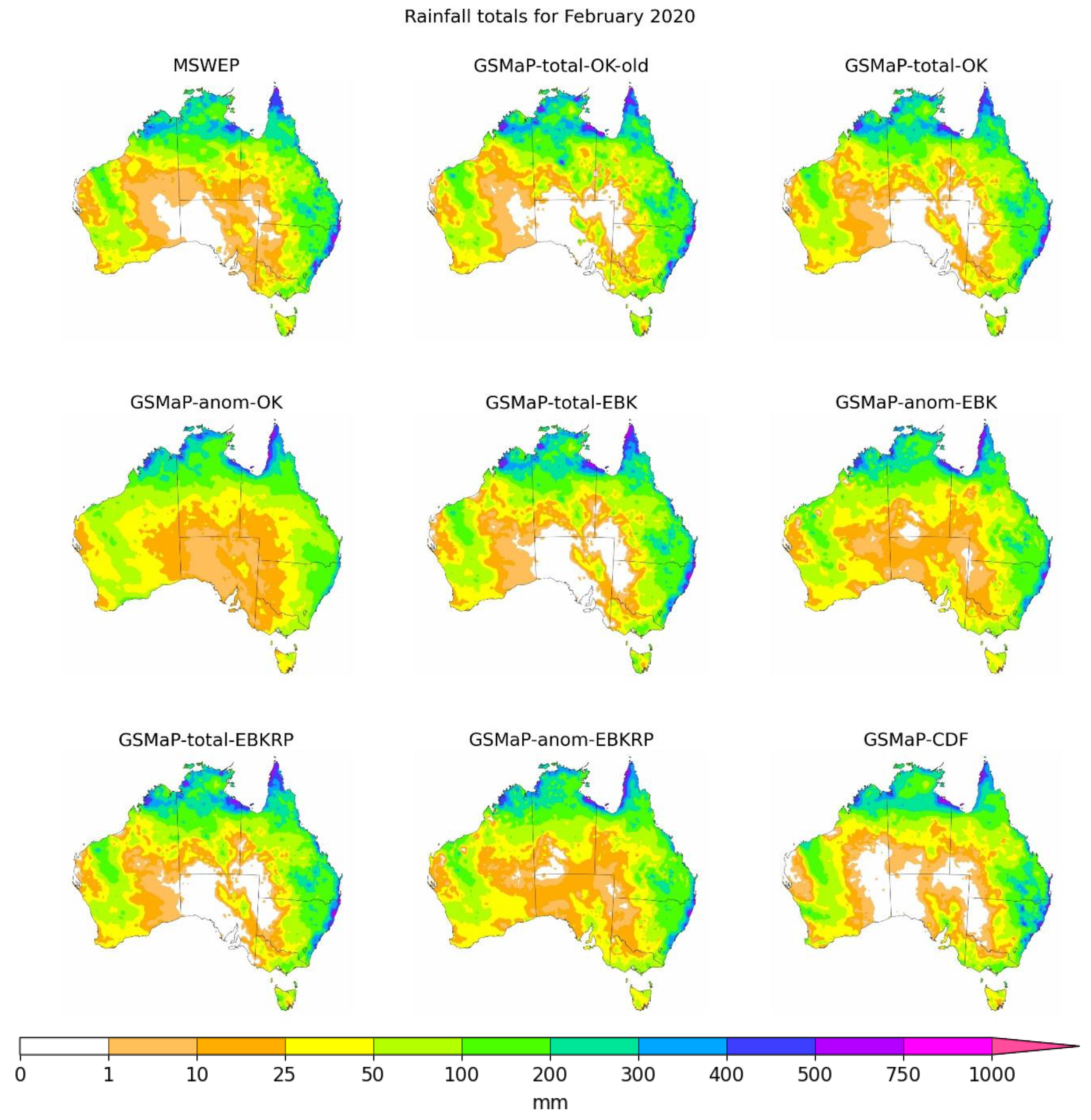
3.1. Corrected Datasets

The results for the corrected datasets are shown in Table 2. Examining the average RMSE and R across the corrected datasets, it was evident that the linear correction-to-totals methods performed the best with average RMSEs between 0.69 to 0.72 and average R values of 0.91. This was followed by the linear correction-to-anomaly methods, with the EBK and EBKRP having a larger edge over OK than what was obtained with a correction to totals. The CDF method was last, but it still outperformed the uncorrected GSMaP.
Using stations as truth, the original method obtained the highest performance. This is expected as this was the only dataset that was corrected to the actual point stations values whereas all the other datasets were corrected to a gridded average. Of note is how the EBK and EBKRP displayed performance that was close despite being corrected to areal averages.
Both the TCA and using MSWEP as truth facilitated a better assessment of performance away from gauges, as well as allowing a comparison to AGCD to be made. Spatial representative errors were also greatly reduced. All the datasets showed reduced biases except for the original dataset, which now had the worst performance. The methods based on the correction to totals performed the best, with the EBK and EBKRP routines being the best. The next best method was anom-EBK, followed by the anom-OK and anom-EBKRP, and lastly by the CDF method.
With MSWEP, AGCD performed the best but there was considerable improvement in the corrected datasets with the RMSE now being only around 15% greater than that of AGCD compared to previously being 80% greater. The correlation also improved with the best R increasing from 0.87 to 0.92, a value only slightly worse than that of AGCD.
The general ranking of the datasets remained the same between the TCA and MSWEP verifications.
The values of σε and correlations obtained from TCA were better, especially the former, which was expected as TCA assumes no error in the truth along with inflation in accuracy due to non-zero correlation between the errors of the datasets. Still, the values were relatively close to each other indicating the appropriateness of TCA as a verification method.
Figure 3 depicts the rainfall totals from each method for an example month of February 2020 with MSWEP included as a reference. This month displays a number of points which are evident across the study period.
In line with the statistical analysis, the total-OK, total-EBKRP, and total-EBK had similar spatial representations, especially the latter two. Compared to total-OK-old, total-OK was more spatially consistent, had less ‘spotty’ artifacts, and had a more controlled representation of high rainfall areas. This resulted in a noticeably improved representation which was not obviously captured in the statistical analysis, as the artifacts were generally a small fraction of the overall domain.
The anom-OK method looked different to anom-EBKRP and anom-EBK, with a similarity between the latter two existing but to a degree less than that in their corresponding totals versions. The inclusion of elevation data in the EBKRP method did not seem to have a noticeable impact, even around the Great Dividing Range, Australia’s key topographical feature.
The anomaly methods could alleviate overinflation for high totals (with anom-EBK and anom-EBKRP being more effective) but introduced spurious rainfall in low-rainfall situations. The rectification of overinflation was not guaranteed with the anomaly methods sometimes producing overinflations of their own. The anomaly methods for EBK and EBKRP were not afflicted by spurious rainfall as often but seemed to have unrealistic missing regions of rainfall, especially over western Tasmania. All the anomaly methods underrepresented rainfall over western Tasmania. The slight negative MB of the anomaly methods suggested that the magnitude of spurious rainfall was offset by the underestimation of high-end totals.
CDF correction appeared to have the most spatially consistent rainfall patterns, including having the least artifacts, but it had problems depicting the correct magnitudes. Underestimation over western Tasmania was again an issue. The EBK and EBKRP methods had slightly fewer artifacts than the OK methods.

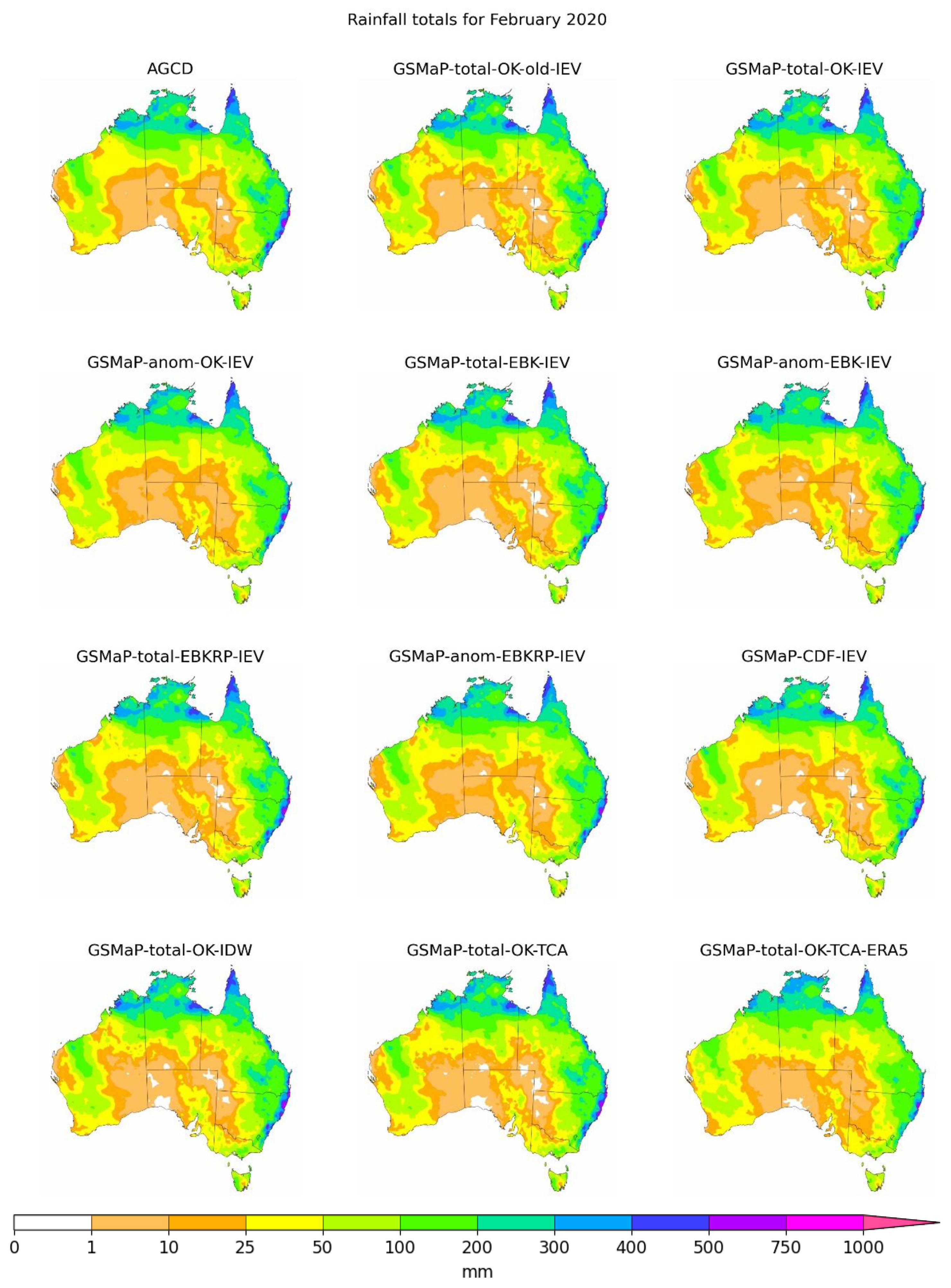
3.2. Blended Datasets

A key result was that the ranking of the corrected datasets could change after the blending process and between blending processes, justifying the decision to trial each blending method with all the corrected datasets, rather than just the best-performing ones.
Importantly, even though the total-EBK had the best overall ranking out of the corrected datasets, the best blended dataset was total-OK-IEV, with total-EBK-IEV coming second. Total-OK-IEV had the best ranking in the MSWEP and the TCA verifications. In the station verification, it was outperformed by the DW-blended datasets as well as by total-EBK-IEV and total-EBKRP-IEV. This suggests it demonstrated the best away-from-station performance in addition to having strong at-station accuracy.
The inverse error variance method yielded the best results, followed by the DW method and then the TCA method. For brevity, only the subset of results for the datasets based on the OK-total and/or IEV methods is shown in Table 3—the full configuration can be found in Appendix C, Table A3. This subset was chosen based on the result of the total-OK-IEV method being the best, along with the variance between the blending techniques and the input-corrected dataset largely being unsubstantial. There is an indirect inclusion of MSWEP in the IEV datasets which would lead to some degree of skill inflation in the MSWEP validation; however, the substitution of MSWEP for ERA5 in the IEV method did not change the result of IEV datasets performing the best in the MSWEP validation.
The various blending techniques all had a harmonising effect on the corrected datasets, with the similarity in the blended products for each technique being relatively high. The degree of harmonisation was less for the TCA blending.
In terms of similarity based on the input dataset, the CDF-corrected dataset yielded the greatest dissimilarity to the others with other methods being fairly similar. The kriging technique matters less than whether correction to totals or anomalies was used.
Figure 4 provides a visual example of the summarised set of blended products, along with AGCD as a reference. Readers are referred back to Figure 3 for the MSWEP totals.
The characteristics of the corrected datasets were transferred to blended products though the harmonisation process meant that the blended products were more similar to each other. For example, the finding that correction via anomaly ratios and by CDF-matching led to smoother representations, but also less accurate magnitudes, also held after the blending process, but the difference to the blended dataset using a ratio to totals was less marked. Nonetheless, it remained as the main point of differentiation, albeit a slight one.
The IEV method was the most effective in reducing spurious rainfall, while TCA was the least effective. For reducing positive bias ‘bullseyes’, both the IEV and DW methods were effective while the TCA method had difficulties. The addition of ERA5 in the TCA-blended method did not necessarily improve results. Only the σε metric from the TCA validation was improved.
Figure 5 shows the period-averaged correlations obtained from the TCA for all the corrected datasets, and the total-OK- and/or IEV-blended variants. GSMaP and AGCD are included for reference. It allows identification of where the correction and blending methods were most effective.
The anom-OK and CDF correction methods were not so effective in the interior of Western Australia, where the gauge network is sparse. The CDF method also did not perform well over central parts of the eastern coastline. The improvement of total-OK over total-OK-old is also clear, especially over the northern coastline. The regions where the method is the weakest appears to be towards the centre of Western Australia, as well as around East Arnhem in Northern Territory.
The similarity of the blending methods is evident. From a glance, only the total-OK-TC-ERA5 method displayed noticeable differences, having slightly weaker correlations across the country than the other blended products. The blending methods improved correlations to a level that was similar to AGCD, with the patch of lower correlation in the centre of Western Australia present in both AGCD and the blended satellite datasets. This is a region of very low gauge density, alluding to the possibility that the blended satellite dataset is still limited, at least to some extent, by the quality of the gauge analysis and its underlying network.

4. Discussion

4.1. Correction Techniques

The use of cell-to-cell correction instead of point-to-cell correction was important in removing stray bullseye artifacts that were a result of large discrepancies due to inconsistent spatial sampling. This was especially true for cases where a gauge value was much higher than its gridded average.
Correction to totals was generally the best at creating a product where the satellite totals were most similar to the observed ones. However, it was also the most prone to artifacts. As described in [16], if GSMaP contained isolated patches of elevated rainfall that were not also present in AGCD, over areas with low rain gauge densities this could lead to incorrect adjustment. If GSMaP totals were less than what were observed at the closest, albeit still faraway gauges, the elevated rainfall patch would end up being greatly exaggerated.
The correction to anomalies dealt better with high totals and also resulted in less artifacts. However, this method struggled with low rainfall totals, generating the greatest amount of spurious light rainfall. This was likely because the final product still contained rainfall from the climatological background. Furthermore, the representation of extreme anomalies could be lost when these anomalies were over poorly observed areas. In these cases, the adjustment was again based on faraway stations where GSMaP and station data were more aligned, resulting in some little adjustments so that the final product resembled the climatology rather than the anomaly.
The CDF method has proved to be effective in past studies, e.g., [50,51]. It created the most realistic-looking representations and was least prone to the incorrect adjustment of isolated anomalies over gauge-sparse areas. This can be attributed to how under this scenario, the other two methods would utilise a faraway station-based adjustment while the CDF method was matched based on the local distributions. Even though the datasets may have been quite different locally in an absolute sense, they could be similar in their relative frequency, reducing the susceptibility of extreme adjustment errors.
However, the CDF method underestimated rainfall during very-low-total scenarios. For dry areas where many totals are zero, the gamma distribution may not be appropriate as zero values have to be excluded during fitting. Sometimes, a lack of adjustment also occurred, including underrepresentation of elevated totals over western Tasmania. It is possible that this was due to the satellite value having a very similar position in its distribution to its station equivalent, resulting in little adjustment. If there was a longer record, this method would likely perform better, as having only 20 years of data can constrain the robustness of the fit, especially for extremes. In [33], the authors increased the amount of data available for fitting by utilising daily data as well as considering surrounding grid cells, likely improving the accuracy derived from this method. However, the method being developed in this study is intended to be limited to monthly data, reducing the resource requirement, and increasing simplicity of use.
The CDF method does not have to rely on the gauge analysis having correct totals, but rather on the frequency of the gauges being more correct. Considering that the representation was relatively similar to that obtained from the linear correction methods, the CDF method could be advantageous for regions with sparser rain gauge networks where the ability to create an accurate rain gauge analysis is more difficult.
The result of a linear correction performing the best has been observed in the literature, including contemporary studies, e.g., [52]. There appears to be a trade-off between better matching at stations and an increased likelihood of artifacts away from stations.
The small amount of variance between the different kriging techniques suggests the assumption of a constant variogram used across the whole domain in OK was generally acceptable. There was not a clear superior variant, with a dependence on the validation dataset used. This can be reconciled with [45], which found EBKRP to be the superior dataset, albeit with only a slight difference to EBK and OK. The differences between EBK and EBKRP did not tend to occur over topography, which was unexpected given elevation was the extra parameter used in EBKRP.

4.2. Blending Techniques

An important result is that the three blending techniques produced a similar representation of rainfall. Considering that all three were derived from considerably different methods (error variance from MSWEP, error variance from a TCA using AGCD and ERA5, and adjustment using distance from stations), this provides confidence that an optimal result (particularly within the technique but also across techniques) was being achieved. It also suggests that obtaining a marked improvement via the use of other blending techniques may be difficult.
The scenario where there was the most difference in the blending techniques was when there was a strong difference in the underlying corrected dataset over a region with sparse rain gauge coverage. The DW-blended method retained this difference, while the other two blended techniques would adjust this difference towards AGCD. The DW method functions as intended in this sense as AGCD should be considered less dependable in these areas and thus weighed less, but at times the corrected satellite dataset contained its own biases which outweighed the effect of reduced reliance on AGCD. As described in Section 4.1, the most problematic scenario for the most performant-corrected dataset (total-OK-IEV) was over-adjusted bullseyes in gauge-sparse regions. The DW method would incorrectly amplify or retain these artifacts, while the other two techniques were able to resolve them.
It was also not a guarantee that the best corrected dataset would result in the best blended dataset—the effect of blending was non-linear. In general, the corrected datasets using a linear correction to totals yielded the best blended dataset with the choice of kriging technique between OK, EBK, and EBKRP not having much effect in this study.
The inclusion of ERA5 data in the TCA-blended dataset did not generally improve performance. The only metric that improved was the σε from the TCA validation, which was expected as the weights were formed from the optimisation of fRMSE. It should also be noted that the TC-ERA5 datasets are more likely to violate the assumption of independence required for TCA, and so the fact that they yielded the lowest TCA error statistics, but worse statistics otherwise, suggests that their TCA results are suspect. A possible reason why performance was not improved could be the introduction of spurious minute rainfall from the use of a greater number of component rainfall datasets, which has a more adverse impact on the correlation metrics than the error ones. The use of additional datasets does not necessarily improve accuracy and requires greater nuance, including the use of a sensible method for determining rain/no-rain cells.
As seen amongst the correction techniques, there was also a trade-off of performance at stations and away from stations among the blending techniques. This is reflected in the validation technique used as well. The station-based verification favoured the DW method due to its explicit inclusion of station data. The MSWEP and TCA validations indicated that the IEV method was the best. Considering that the MSWEP and TCA validations are more generalised and evaluate performance both at and away from stations, they are likely a better indicator of the overall performance of datasets. The IEV-blending method also performed relatively well in the station validation, being the best non-DW method evaluated.

5. Conclusions

Gauge analyses possess high uncertainty in gauge-sparse regions and while alternative data sources like satellites can provide estimates for these areas, their indirect form of estimation means their accuracy is less than gauge analyses where stations exist. By combining satellite and gauge data, a better dataset that takes advantage of the complementary nature of both sources can be produced. This study evaluated the efficacy of various configurations of correction and blending techniques. The correction techniques trialled were linear correction to totals, linear correction to anomalies, and CDF matching. The blending techniques tested were based on inverse error variance using MSWEP as truth, a distance-weighted approach, and a triple collocation analysis-weighting scheme using GSMaP, AGCD, and ERA5. The main findings are as follows:
  • The most performant correction technique in this study was a linear correction to totals. The choice of kriging technique did not have a strong impact, with EBK slightly outperforming EBKRP and OK;
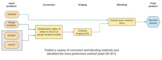
  • The most performant blending technique was an inverse error variance blending technique using a GSMaP dataset linearly corrected to totals. All the blending techniques tested were able to improve the underlying corrected dataset, having a harmonising effect that greatly reduced the differences between the corrected datasets. The improvement was non-linear, resulting in the total-OK-IEV-blended dataset performing the best generally;
  • The validation technique used is important, as station-based validation favoured DW-blended datasets while the more general TCA and MSWEP validations favoured the IEV-blended datasets. Triple collocation analysis using satellite data, SM2R, and ERA5 as the triplet yielded results consistent with a traditional comparison to MSWEP, highlighting the versatility of the technique;
  • The trade-off between at-station and away-from-station performance was clear. For the correction techniques, the CDF method traded at-station performance for away-from-station performance. For the blending techniques, the DW method traded away-from-station performance for at-station performance. This made them complementary to each other. Likewise, the linear correction methods were complementary to the IEV blending methods.
The results of having three different blending techniques yield a similar representation of rainfall, suggesting that the blended result obtained in this study is close to being optimal. When both at-station and away-from-station performance is considered, total-OK-IEV performed the best. The effectiveness of this method over a domain with much fewer rain gauges is an important future research topic as the rain gauge analysis is an important ingredient in this method.

Author Contributions

Conceptualisation, Z.-W.C., Y.K., A.B.W., S.C. and C.S.; methodology, Z.-W.C. and Y.K.; software, Z.-W.C.; validation, Z.-W.C.; formal analysis, Z.-W.C.; investigation, Z.-W.C.; resources, Z.-W.C.; data curation, Z.-W.C.; writing—original draft preparation, Z.-W.C.; writing—review and editing, Z.-W.C., Y.K., A.B.W., S.C. and C.S.; visualisation, Z.-W.C., supervision, Z.-W.C., Y.K., A.B.W., S.C. and C.S.; project administration, Z.-W.C. and Y.K. All authors have read and agreed to the published version of the manuscript.

Funding

This research was supported by the World Meteorological Organization through “Weather and Climate Early Warning System for Papua New Guinea (CREWS-PNG)” project 20170888.

Data Availability Statement

GSMaP data were provided by EORC, JAXA. CMORPH data were provided by CPC, NOAA. AGCD and station gauge data were provided by the Bureau of Meteorology. Contains modified Copernicus Climate Change Service Information (2019). Neither the European Commission nor ECMWF is responsible for any use that may be made of the Copernicus Information or Data it contains. MSWEP data were provided by GloH2O.

Acknowledgments

We are grateful to colleagues from the Climate Monitoring and Long-Range Forecasts sections of the Bureau of Meteorology for their helpful advice and guidance. Three anonymous reviewers provided valuable comments which helped us to improve the quality of the initial manuscript.

Conflicts of Interest

The authors declare no conflict of interest.

Appendix A

The assumptions were generally met and TCA should be considered appropriate. Full satisfaction was not expected given several factors which would make it virtually impossible. For example, some correlation in the errors is expected due to the use of an imperfect truth which would result in a common bias amongst all the datasets.
  • Stationarity of the data (no autocorrelation).
An Augmented Dickey–Fuller Test (ADFT) was performed on the monthly time series of each of the TCA datasets over the study domain (the OK-total-IEV-blended dataset is used as an example). The ADFT tests the null hypothesis that the dataset has a unit root (H0), with more negative values indicating a greater confidence in the stationarity of the dataset [53]. SM2R, GSMaP, and ERA5 exhibited very high confidence of being stationary, with H0 being rejected at greater than a 99% level. AGCD along with the corrected and blended satellite datasets demonstrated a greater degree of non-stationarity and could only be rejected at a greater than 20% level;
2.
The datasets can be linearly related to each other.
The linear correlation of the monthly time series to that of ERA5 and SM2R was computed. All the datasets showed a high level of linear correlation, ranging from 0.8 to 0.9;
3.
Orthogonality of errors (their expected sum is zero).
A monthly time series of the domain-averaged error for each dataset was computed using MSWEP as truth. This was then compared against the mean of the data to see how large the error was. SM2R had the largest proportion (around 7%), but for other datasets the ratio was 5% or less;
4.
There is no cross-correlation amongst the errors of the datasets, as well as with the truth.
A linear correlation was performed on the time series of the errors to that of ERA5 and SM2R. Correlations were generally low. ERA5 correlations were higher, though the highest correlation was only around 0.36. Table A1 below contains the full results.
Table A1. Metrics testing whether the assumptions required for TCA are satisfied.
DatasetADF Statisticp-ValueRatio of Bias to Mean (%)R to SM2RR to ERA5R to SM2R (Bias)R to ERA5 (Bias)
SM2R−11.080.00−7.07-0.90-0.18
ERA5−7.920.00−5.000.90-0.18-
AGCD−2.690.082.180.890.900.24−0.37
GSMaP−11.860.00−0.670.830.850.120.32
GSMaP OK-total−2.270.181.390.880.900.170.36
GSMaP OK-total-IEV−2.350.61.580.890.920.190.36

Appendix B

Six models were tested—Generalised Exponential, Generalised Extreme, Pearson III, Generalised Gamma, Inverse Gaussian, and Inverse Gamma. A CDF corresponding to these models was fitted to all the values across the domain and the entire period. Values were masked to be only over land. Both satellite and AGCD data were fitted. The fitting was then repeated for a larger set of AGCD values, spanning 100 years from 1921 to 2021 to check if the results varied for a longer record. This could not be achieved for the satellite data due to its comparatively shorter record.
The Kolmogorov–Smirnov (K-S) test was used to evaluate goodness-of-fit. The K-S test calculates the distance between the empirical distribution function of the sample and a reference CDF, with lower values indicating a better fit [54]. The set of values used to fit the CDFs was used as the sample while each of the fitted CDFs was used as the reference. The results are shown below in Table A2.
Table A2. Kolmogorov–Smirnov (K-S) goodness-of-fit test for various distributions.
ModelSatelliteAGCDAGCD (100 Years)
Generalised Exponential0.250.170.17
Generalised Extreme0.290.140.14
Pearson III0.250.090.09
Generalised Gamma0.250.080.08
Inverse Gaussian0.280.100.10
Inverse Gamma0.430.150.15
Gamma0.290.080.08
The generalised gamma model had the best performance, followed by the gamma model. Both are based on the same distribution, but the former includes an additional parameter. The generalised gamma model increased the generation time by an order of 100. Considering this, the gamma model was chosen as it showed similarly good performance.

Appendix C

The full configuration of verification statistics for blended datasets with AGCD included as a reference is presented in Table A3.
Table A3. Verification results for all corrected and blended datasets in this study.
StationMSWEPTCAOverall
RMSERRankRMSERRankσεRRankRank (Mean)
GSMaP-total-OK-IEV-old0.620.9690.570.9470.440.931610.3
GSMaP-total-OK-IEV0.660.95120.540.9520.400.9416.2
GSMaP-anom-OK-IEV0.690.95130.540.9510.400.9426.7
GSMaP-total -EBK-IEV0.640.95100.550.9430.420.9436.8
GSMaP-anom-EBK-IEV0.720.94180.570.9440.400.93610.5
GSMaP-total-EBKRP-IEV0.640.95110.560.9450.410.9438.2
GSMaP-anom-EBKRP-IEV0.720.94170.570.9480.400.93310.7
GSMaP-CDF-IEV0.700.95150.610.93150.450.932216.2
GSMaP-total-OK-DW0.600.9640.600.9490.450.9399.3
GSMaP-anom-OK-DW0.600.9680.580.9450.440.922511.3
GSMaP-total-EBK-DW0.600.9620.640.93160.460.932112.2
GSMaP-anom-EBK-DW0.600.9640.600.94100.450.922511.7
GSMaP-total-EBKRP-DW0.600.9630.660.92210.460.932314.3
GSMaP-anom-EBKRP-DW0.600.9660.640.93170.460.922815.5
GSMaP-CDF-DW0.600.9660.750.90220.570.912918.8
GSMaP-total-OK-TC0.720.94180.600.94100.440.93713.2
GSMaP-total-anom-TC0.770.93220.610.93120.440.921817.2
GSMaP-total-EBK-TC0.690.94140.620.93130.450.931815.0
GSMaP-anom-EBK-TC0.740.94200.620.93140.440.921716.8
GSMaP-total-EBKRP-TC0.700.94160.630.93170.450.932017.0
GSMaP-anom-EBKRP-TC0.740.94210.640.92200.450.922320.0
GSMaP-CDF-TC0.790.93230.750.90230.570.912924.8
GSMaP-total-OK-TC-ERA51.280.76261.230.68240.320.92821.0
GSMaP-anom-OK-TC-ERA51.340.74301.270.66300.310.911525.0
GSMaP-total-EBK-TC-ERA51.270.76241.240.68250.320.921221.3
GSMaP-anom-EBK-TC-ERA51.320.75281.270.66290.310.91923.7
GSMaP-total-EBKRP-TC-ERA51.270.76241.240.67260.320.921221.5
GSMaP-anom-EBKRP-TC-ERA51.320.75281.270.66280.320.911223.7
GSMaP-CDF-TC-ERA51.300.75271.260.66270.410.892725.0
AGCD0.440.9810.620.92190.420.93911.2

References

  1. Mukabutera, A.; Thomson, D.; Murray, M.; Basinga, P.; Nyirazinyoye, L.; Atwood, S.; Savage, K.P.; Ngirimana, A.; Hedt-Gauthier, B.L. Rainfall variation and child health: Effect of rainfall on diarrhea among under 5 children in Rwanda, 2010. BMC Public Health 2016, 16, 731. [Google Scholar] [CrossRef] [Green Version]
  2. Bhardwaj, J.; Kuleshov, Y.; Watkins, A.B.; Aitkenhead, I.; Asghari, A. Building capacity for a user-centred Integrated Early Warning System (I-EWS) for drought in the Northern Murray-Darling Basin. Nat. Hazards 2021, 107, 97–122. [Google Scholar] [CrossRef]
  3. Mishra, A.K.; Özger, M.; Singh, V.P. Association between Uncertainties in Meteorological Variables and Water-Resources Planning for the State of Texas. J. Hydrol. Eng. 2011, 16, 984–999. [Google Scholar] [CrossRef]
  4. Gebregiorgis, A.S.; Hossain, F. Understanding the dependence of satellite rainfall uncertainty on topography and climate for hydrologic model simulation. IEEE Trans. Geosci. Remote Sens. 2013, 51, 704–718. [Google Scholar] [CrossRef]
  5. Milly, P.C.D.; Dunne, K.A.; Vecchia, A.V. Global pattern of trends in streamflow and water availability in a changing climate. Nature 2005, 438, 347–350. [Google Scholar] [CrossRef]
  6. Beck, H.E.; Wood, E.F.; Pan, M.; Fisher, C.K.; Miralles, D.G.; Van Dijk, A.I.J.M.; McVicar, T.R.; Adler, R.F. MSWep v2 Global 3-hourly 0.1° precipitation: Methodology and quantitative assessment. Bull. Am. Meteorol. Soc. 2019, 100, 473–500. [Google Scholar] [CrossRef] [Green Version]
  7. Michelson, D.B. Systematic correction of precipitation gauge observations using analyzed meteorological variables. J. Hydrol. 2004, 290, 161–177. [Google Scholar] [CrossRef]
  8. Contractor, S.; Alexander, L.V.; Donat, M.G.; Herold, N. How Well Do Gridded Datasets of Observed Daily Precipitation Compare over Australia? Adv. Meteorol. 2015, 2015, 325718. [Google Scholar] [CrossRef] [Green Version]
  9. Hofstra, N.; New, M.; McSweeney, C. The influence of interpolation and station network density on the distributions and trends of climate variables in gridded daily data. Clim. Dyn. 2010, 35, 841–858. [Google Scholar] [CrossRef]
  10. New, M.; Todd, M.; Hulme, M.; Jones, P. Precipitation measurements and trends in the twentieth century. Int. J. Climatol. 2001, 21, 1889–1922. [Google Scholar] [CrossRef]
  11. Habib, E.; Krajewski, W.F.; Ciach, G.J. Estimation of Rainfall Interstation Correlation. J. Hydrometeorol. 2001, 2, 621–629. [Google Scholar] [CrossRef]
  12. Kidd, C.; Becker, A.; Huffman, G.J.; Muller, C.L.; Joe, P.; Skofronick-Jackson, G.; Kirschbaum, D.B. So, how much of the Earth’s surface is covered by rain gauges? Bull. Am. Meteorol. Soc. 2017, 98, 69–78. [Google Scholar] [CrossRef]
  13. Ensor, L.A.; Robeson, S.M. Statistical characteristics of daily precipitation: Comparisons of gridded and point datasets. J. Appl. Meteorol. Climatol. 2008, 47, 2468–2476. [Google Scholar] [CrossRef]
  14. Xie, P.; Arkin, P.A. Global Precipitation: A 17-Year Monthly Analysis Based on Gauge Observations, Satellite Estimates, and Numerical Model Outputs. Bull. Am. Meteorol. Soc. 1997, 78, 2539–2558. [Google Scholar] [CrossRef]
  15. Dong, J.; Lei, F.; Wei, L. Triple Collocation Based Multi-Source Precipitation Merging. Front. Water 2020, 2, 1. [Google Scholar] [CrossRef]
  16. Chua, Z.-W.; Kuleshov, Y.; Watkins, A.; Choy, S.; Sun, C. Developing a blended satellite-gauge rainfall dataset over Australia. J. Hydrometeorol. 2022; under review. [Google Scholar]
  17. Stoffelen, A. Toward the true near-surface wind speed: Error modeling and calibration using triple collocation. J. Geophys. Res. Ocean 1998, 103, 7755–7766. [Google Scholar] [CrossRef]
  18. McColl, K.A.; Vogelzang, J.; Konings, A.G.; Entekhabi, D.; Piles, M.; Stoffelen, A. Extended triple collocation: Estimating errors and correlation coefficients with respect to an unknown target. Geophys. Res. Lett. 2014, 41, 6229–6236. [Google Scholar] [CrossRef] [Green Version]
  19. Roebeling, R.A.; Wolters, E.L.A.; Meirink, J.F.; Leijnse, H. Triple collocation of summer precipitation retrievals from SEVIRI over europe with gridded rain gauge and weather radar data. J. Hydrometeorol. 2012, 13, 1552–1566. [Google Scholar] [CrossRef]
  20. Alemohammad, S.H.; McColl, K.A.; Konings, A.G.; Entekhabi, D.; Stoffelen, A. Characterization of precipitation product errors across the United States using multiplicative triple collocation. Hydrol. Earth Syst. Sci. 2015, 19, 3489–3503. [Google Scholar] [CrossRef] [Green Version]
  21. Massari, C.; Crow, W.; Brocca, L. An assessment of the performance of global rainfall estimates without ground-based observations. Hydrol. Earth Syst. Sci. 2017, 21, 4347–4361. [Google Scholar] [CrossRef] [Green Version]
  22. Mega, T.; Ushio, T.; Matsuda, T.; Kubota, T.; Kachi, M.; Oki, R. Gauge-Adjusted Global Satellite Mapping of Precipitation. IEEE Trans. Geosci. Remote Sens. 2019, 57, 1928–1935. [Google Scholar] [CrossRef]
  23. Ebert, E.E.; Janowiak, J.E.; Kidd, C. Comparison of near-real-time precipitation estimates from satellite observations and numerical models. Bull. Am. Meteorol. Soc. 2007, 88, 47–64. [Google Scholar] [CrossRef] [Green Version]
  24. Dinku, T.; Ceccato, P.; Cressman, K.; Connor, S.J. Evaluating detection skills of satellite rainfall estimates over desert locust recession regions. J. Appl. Meteorol. Climatol. 2010, 49, 1322–1332. [Google Scholar] [CrossRef]
  25. Hersbach, H.; Bell, B.; Berrisford, P.; Hirahara, S.; Horányi, A.; Muñoz-Sabater, J.; Nicolas, J.; Peubey, C.; Radu, R.; Schepers, D.; et al. The ERA5 global reanalysis. Q. J. R. Meteorol. Soc. 2020, 146, 1999–2049. [Google Scholar] [CrossRef]
  26. Bosilovich, M.G.; Chen, J.; Robertson, F.R.; Adler, R.F. Evaluation of global precipitation in reanalyses. J. Appl. Meteorol. Climatol. 2008, 47, 2279–2299. [Google Scholar] [CrossRef]
  27. Evans, A.; Jones, D.; Smalley, R.; Lellyett, S. An Enhanced Gridded Rainfall Dataset Scheme for Australia; Bureau of Meteorology: Melbourne, Australia, 2020; ISBN 978-1-925738-12-4. [Google Scholar]
  28. Brocca, L.; Filippucci, P.; Hahn, S.; Ciabatta, L.; Massari, C.; Camici, S.; Schüller, L.; Bojkov, B.; Wagner, W. SM2RAIN-ASCAT (2007–2018): Global daily satellite rainfall data from ASCAT soil moisture observations. Earth Syst. Sci. Data 2019, 11, 1583–1601. [Google Scholar] [CrossRef] [Green Version]
  29. Wagner, W.; Hahn, S.; Kidd, R.; Melzer, T.; Bartalis, Z.; Hasenauer, S.; Figa-Saldaña, J.; De Rosnay, P.; Jann, A.; Schneider, S.; et al. The ASCAT soil moisture product: A review of its specifications, validation results, and emerging applications. Meteorol. Zeitschrift 2013, 22, 5–33. [Google Scholar] [CrossRef] [Green Version]
  30. Huffman, G.J.; Bolvin, D.T.; Braithwaite, D.; Hsu, K.L.; Joyce, R.J.; Kidd, C.; Nelkin, E.J.; Sorooshian, S.; Stocker, E.F.; Tan, J.; et al. Integrated Multi-satellite Retrievals for the Global Precipitation Measurement (GPM) Mission (IMERG). In Advances in Global Change Research; Springer: Berlin/Heidelberg, Germany, 2020; Volume 67, pp. 343–353. [Google Scholar]
  31. Rudolf, B.; Hauschild, H.; Rueth, W.; Schneider, U. Terrestrial Precipitation Analysis: Operational Method and Required Density of Point Measurements. In Global Precipitations and Climate Change; Springer: Berlin/Heidelberg, Germany, 1994; pp. 173–186. [Google Scholar]
  32. Chen, M.; Xie, P.; Janowiak, J.E. Global land precipitation: A 50-yr monthly analysis based on gauge observations. J. Hydrometeorol. 2002, 3, 249–266. [Google Scholar] [CrossRef]
  33. Xie, P.; Xiong, A.Y. A conceptual model for constructing high-resolution gauge-satellite merged precipitation analyses. J. Geophys. Res. Atmos. 2011, 116, D21106. [Google Scholar] [CrossRef]
  34. Mastrantonas, N.; Bhattacharya, B.; Shibuo, Y.; Rasmy, M.; Espinoza-Dávalos, G.; Solomatine, D. Evaluating the benefits of merging near-real-time satellite precipitation products: A case study in the Kinu basin region, Japan. J. Hydrometeorol. 2019, 20, 1213–1233. [Google Scholar] [CrossRef]
  35. Piani, C.; Haerter, J.O.; Coppola, E. Statistical bias correction for daily precipitation in regional climate models over Europe. Theor. Appl. Climatol. 2010, 99, 187–192. [Google Scholar] [CrossRef] [Green Version]
  36. Ines, A.V.M.; Hansen, J.W. Bias correction of daily GCM rainfall for crop simulation studies. Agric. For. Meteorol. 2006, 138, 44–53. [Google Scholar] [CrossRef] [Green Version]
  37. Pombo, S.; de Oliveira, R.P. Evaluation of extreme precipitation estimates from TRMM in Angola. J. Hydrol. 2015, 523, 663–679. [Google Scholar] [CrossRef]
  38. Alam, M.A.; Emura, K.; Farnham, C.; Yuan, J. Best-fit probability distributions and return periods for maximum monthly rainfall in Bangladesh. Climate 2018, 6, 9. [Google Scholar] [CrossRef] [Green Version]
  39. Yue, S.; Hashino, M. Probability distribution of annual, seasonal and monthly precipitation in Japan. Hydrol. Sci. J. 2007, 52, 863–877. [Google Scholar] [CrossRef]
  40. Mamoon, A.A.; Rahman, A. Selection of the best fit probability distribution in rainfall frequency analysis for Qatar. Nat. Hazards 2017, 86, 281–296. [Google Scholar] [CrossRef]
  41. Enayati, M.; Bozorg-Haddad, O.; Bazrafshan, J.; Hejabi, S.; Chu, X. Bias correction capabilities of quantile mapping methods for rainfall and temperature variables. J. Water Clim. Chang. 2021, 12, 401–419. [Google Scholar] [CrossRef]
  42. Becker, A.; Finger, P.; Meyer-Christoffer, A.; Rudolf, B.; Schamm, K.; Schneider, U.; Ziese, M. A description of the global land-surface precipitation data products of the Global Precipitation Climatology Centre with sample applications including centennial (trend) analysis from 1901-present. Earth Syst. Sci. Data 2013, 5, 71–99. [Google Scholar] [CrossRef] [Green Version]
  43. Funk, C.; Peterson, P.; Landsfeld, M.; Pedreros, D.; Verdin, J.; Shukla, S.; Husak, G.; Rowland, J.; Harrison, L.; Hoell, A.; et al. The climate hazards infrared precipitation with stations—A new environmental record for monitoring extremes. Sci. Data 2015, 2, 150066. [Google Scholar] [CrossRef] [Green Version]
  44. Wackernagel, H. Multivariate Geostatistics: An Introduction with Applications; Multivar. geostatistics an Introd. with Appl; Springer: Berlin/Heidelberg, Germany, 1995. [Google Scholar] [CrossRef]
  45. Ali, G.; Sajjad, M.; Kanwal, S.; Xiao, T.; Khalid, S.; Shoaib, F.; Gul, H.N. Spatial–temporal characterization of rainfall in Pakistan during the past half-century (1961–2020). Sci. Rep. 2021, 11, 6935. [Google Scholar] [CrossRef] [PubMed]
  46. Frazier, A.G.; Giambelluca, T.W.; Diaz, H.F.; Needham, H.L. Comparison of geostatistical approaches to spatially interpolate month-year rainfall for the Hawaiian Islands. Int. J. Climatol. 2016, 36, 1459–1470. [Google Scholar] [CrossRef] [Green Version]
  47. Adhikary, S.K.; Muttil, N.; Yilmaz, A.G. Cokriging for enhanced spatial interpolation of rainfall in two Australian catchments. Hydrol. Process. 2017, 31, 2143–2161. [Google Scholar] [CrossRef] [Green Version]
  48. Gribov, A.; Krivoruchko, K. Empirical Bayesian kriging implementation and usage. Sci. Total Environ. 2020, 722, 137290. [Google Scholar] [CrossRef] [PubMed]
  49. Gupta, A.; Kamble, T.; Machiwal, D. Comparison of ordinary and Bayesian kriging techniques in depicting rainfall variability in arid and semi-arid regions of north-west India. Environ. Earth Sci. 2017, 76, 512. [Google Scholar] [CrossRef]
  50. Valdés-Pineda, R.; Demaría, E.; Valdés, J.; Wi, S.; Serrat-Capdevilla, A. Bias correction of daily satellite-based rainfall estimates for hydrologic forecasting in the Upper Zambezi, Africa. Hydrol. Earth Syst. Sci. Discuss. 2016, 1–28. [Google Scholar] [CrossRef] [Green Version]
  51. Katiraie-Boroujerdy, P.S.; Naeini, M.R.; Asanjan, A.A.; Chavoshian, A.; Hsu, K.L.; Sorooshian, S. Bias correction of satellite-based precipitation estimations using quantile mapping approach in different climate regions of Iran. Remote Sens. 2020, 12, 2102. [Google Scholar] [CrossRef]
  52. Gumindoga, W.; Rientjes, T.H.M.; Tamiru Haile, A.; Makurira, H.; Reggiani, P. Performance of bias-correction schemes for CMORPH rainfall estimates in the Zambezi River basin. Hydrol. Earth Syst. Sci. 2019, 23, 2915–2938. [Google Scholar] [CrossRef] [Green Version]
  53. Chatfield, C.; Fuller, W.A. Introduction to Statistical Time Series. J. R. Stat. Soc. Ser. A 1977, 140, 379. [Google Scholar] [CrossRef]
  54. Massey, F.J. The Kolmogorov-Smirnov Test for Goodness of Fit. J. Am. Stat. Assoc. 1951, 46, 68–78. [Google Scholar] [CrossRef]
Figure 1. Typical rain gauge network coverage in Australia. Rain gauge locations are depicted by the blue dots while topography is represented by the shading. The main topographical feature is the Great Dividing Range along the east coast of the country.
Remotesensing 14 00261 g001
Figure 2. Datasets and processes involved in creating the corrected and blended datasets.
Remotesensing 14 00261 g002
Figure 3. Corrected rainfall analyses for February 2020.
Remotesensing 14 00261 g003
Figure 4. Blended rainfall analyses for February 2020.
Remotesensing 14 00261 g004
Figure 5. Correlations obtained using triple collocation analysis for corrected and blended datasets.
Remotesensing 14 00261 g005
Table 1. Details on datasets used in this study for creation of the blended dataset, as well as for validation.
Dataset and Data SourceExplanationBiasesResolution and Domain
Global Satellite Mapping of Precipitation (GSMaP) from Japan Aerospace Exploration Agency (JAXA), microwave-based estimates from satellites [22].A rain rate is estimated from the emission and change in the scattering of microwaves due to precipitation. These microwave estimates are advected using cloud motion vectors to increase their spatiotemporal coverage.Measurement error from the sensors and the reliance on algorithms to obtain a rain rate. The algorithms are known to have a deficiency over topography and coastal boundaries. The detection of light rain from warm clouds [23] and sub-cloud evaporation of rainfall in arid environments [24] are also known problems.0.1° × 0.1° global from 60° S to 60° N, hourly
ERA5 from the European Centre for Medium-Range Forecast (ECMWF), model reanalysis [25].Created using 4D-Var assimilation of observations into their weather forecast model, the Integrated Forecast System (IFS). Assimilation does not include rainfall from gauges but gauge-corrected radar over the United States of America (US) as well as satellite radiances and atmospheric motion vectors are ingested.Biases arise from the observations ingested, as well as from the assimilation and modelling processes with reduced observations leading to a deterioration in quality [26]. In line with other reanalyses, ERA5 has reduced variability, with spurious low-end rainfall being a contributing factor [6].0.1° × 0.1° global, hourly
Multi-Source Weighted Ensemble Product (MSWEP) from GloH2O, gauge-reanalysis-satellite-blended dataset [6].Formed from a blend of gauge, satellite, and reanalysis data. The weights for each dataset are based on their correlation to rain gauge data.Inherent biases from source datasets as well as that introduced from the blending algorithm.0.1° × 0.1° global, 3 hourly
Australian Gridded Climate Dataset (AGCD) from Bureau of Meteorology (BOM), gauge analysis [27].Created using optimal interpolation. Station climatology is used to form the background field onto which incremental adjustments are made using monthly observations.The density of rain gauges presents the largest control on the quality of the analysis, with the interpolation method generally having a much less significant effect [9]. Quality of the gauge data is also a factor, though quality control is performed on input stations prior to and during interpolation [27].0.01° × 0.01° over Australia, monthly
Australian Data Archive for Meteorology (ADAM) rain gauges from BOM.Contains the data of over 6700 rain gauges across the country. Only stations which had a quality flag of less than six (i.e., checked as not being suspect) were used in this study.As described in Section 1.Number of stations ranged from 4346 to 6664 over the study period, daily
Soil Moisture to Rain (SM2R) from ESA Climate Change Initiative (CCI), rainfall analysis derived from satellite soil moisture data [28].Based on soil moisture estimates from scatterometers on board the MetOp satellites to infer accumulated rainfall. This ‘bottom-up’ approach contrasts with the ‘top-down’ approach of microwave estimates which estimate instantaneous rain rates from upwelling radiation.Performance degrades over arid areas, frozen soils, tropical rainforests, and topography as the algorithm cannot directly account for the changes in backscatter caused by these surfaces [29]. S2MR has known biases with spurious rainfall due to high-frequency soil moisture fluctuations and underestimation of high-end rainfall [28]. A triple collocation study performed globally demonstrated the performance of SM2R was similar and at times superior to ERA5 and IMERG (Integrated Multi-satellite Retrievals for GPM; see [30] for details) over gauge-sparse regions of the world, including parts of Australia [28].0.25° × 0.25° global, daily
Table 2. Verification statistics for the corrected datasets with GSMaP included as a reference.
StationMSWEPTCAOverall
RMSERRankRMSERRankσεRRankMean Rank
GSMaP1.560.791.010.8280.780.7998.5
GSMaP-total-OK-old0.810.9211.110.8770.740.8764.8
GSMaP-total-OK0.910.8940.720.9110.540.9132.8
GSMaP-anom-OK1.240.8170.880.8660.630.8477
GSMaP-total-EBK0.810.9120.720.9210.530.9211.5
GSMaP-anom-EBK1.090.8550.820.8740.560.8844.5
GSMaP-total-EBKRP0.830.9130.740.930.540.9122.7
GSMaP-anom-EBKRP1.10.8560.860.8650.590.8845.3
GSMaP-CDF1.320.8171.080.8280.880.8587.8
AGCD0.440.9810.620.92190.420.93911.2
Table 3. Verification statistics for blended datasets with AGCD included as a reference.
StationMSWEPTCAOverall
RMSERRankRMSERRankσεRRankRank (Mean)
GSMaP-total-OK-IEV-old0.620.9690.570.9470.440.931610.3
GSMaP-total-OK-IEV0.660.95120.540.9520.400.9416.2
GSMaP-anom-OK-IEV0.690.95130.540.9510.400.9426.7
GSMaP-total-EBK-IEV0.640.95100.550.9430.420.9436.8
GSMaP-anom-EBK-IEV0.720.94180.570.9440.400.93610.5
GSMaP-total-EBKRP-IEV0.640.95110.560.9450.410.9438.2
GSMaP-anom-EBKRP-IEV0.720.94170.570.9480.400.93310.7
GSMaP-total-OK-DW0.600.9640.600.9490.450.9399.3
GSMaP-total-OK-TC0.720.94180.600.94100.440.93713.2
GSMaP-total-OK-TC-ERA51.280.76261.230.68240.320.92821.0
AGCD0.440.9810.620.92190.420.93911.2
Publisher’s Note: MDPI stays neutral with regard to jurisdictional claims in published maps and institutional affiliations.

