Article

Characteristics of Snow Depth and Snow Phenology in the High Latitudes and High Altitudes of the Northern Hemisphere from 1988 to 2018

1
Key Laboratory of Remote Sensing of Gansu Province, Heihe Remote Sensing Experimental Research Station, Northwest Institute of Eco-Environment and Resources, Chinese Academy of Sciences, Lanzhou 730000, China
2
National Tibetan Plateau Data Center, State Key Laboratory of Tibetan Plateau Earth System, Environment and Resources, Institute of Tibetan Plateau Research, Chinese Academy of Sciences, Beijing, 100101, China
3
College of Resources and Environment, University of Chinese Academy of Sciences, Beijing 100049, China
4
National Forestry and Grassland Administration Key Laboratory of Forest Resource Conservation and Ecological Safety on the Upper Reaches of the Yangtze River, Sichuan Province Key Laboratory of Ecological Forestry Engineering on the Upper Reaches of the Yangtze River, College of Forestry, Sichuan Agricultural University, Chengdu 611130, China
*
Author to whom correspondence should be addressed.
Remote Sens. 2022, 14(19), 5057; https://doi.org/10.3390/rs14195057
Submission received: 2 September 2022 / Revised: 28 September 2022 / Accepted: 5 October 2022 / Published: 10 October 2022

Abstract

:
Snow cover is an important part of the Earth’s surface and its changes affect local and even global climates due to the high albedo and heat insulation. However, it is difficult to directly compare the results of previous studies on changes in snow cover in the Northern Hemisphere mainland (NH) due to the use of different datasets, research methods, or study periods, and a lack comparison in terms of the differences and similarities at high latitudes and high altitudes. By using snow depth datasets, we analyzed the spatio-temporal distributions and variations in snow depth (SD) and snow phenology (SP) in the NH and nine typical areas. This study revealed that SD in the NH generally decreased significantly (p < 0.01) from 1988 to 2018, with a rate of −0.55 cm/decade. Changes in SD were insignificant at high altitudes, but significant decreases were found at high latitudes. With regard to SP, the snow cover onset day (SCOD) advanced in 31.57% of the NH and was delayed in 21.10% of the NH. In typical areas such as the Rocky Mountains, the West Siberian Plain, and the Central Siberian Plateau, the SCOD presented significant advancing trends, while a significant delay was the trend observed in the Eastern European Plain. The snow cover end day (SCED) advanced in 37.29% of the NH and was delayed in 14.77% of the NH. Negative SCED trends were found in most typical areas. The snow cover duration (SCD) and snow season length (SSL) showed significant positive trends in the Rocky Mountains, while significant negative trends were found in the Qinghai–Tibet Plateau. The results of this comprehensive comparison showed that most typical areas were characterized by decreased SD, advanced SCOD and SCED, and insignificantly increasing SCD and SSL trends. The SCD and SSL values were similar at high latitudes, while the SSL value was larger than the SCD value at high altitudes. The SD exhibited similar interannual fluctuation characteristics as the SCD and SSL in each typical area. The SCD and SSL increased (decreased) with advanced (delayed) SCODs.

Graphical Abstract

1. Introduction

Snow cover, a crucial element of the cryosphere, plays a vital role in the climate system and the global hydrological circulation system because the high albedo and heat insulation associated with snow cover alter the near-surface temperatures and surface energy budget of Earth [1,2,3,4,5]. Meltwater from seasonal snow cover is an indispensable water resource, feeding 17% of the global population [4,6]. In addition, snow cover is closely linked to the human economy through the development of winter tourism, such as skiing and other sports performed in mountainous areas [7,8,9]. Snow phenology (SP) parameters such as the snow cover onset day (SCOD), snow cover end day (SCED), snow cover duration (SCD), and snow season length (SSL) are effective variables used to reflect snow cover changes caused by climate change and have become an increasingly valuable climate change indicators in recent decades [10,11,12]. According to previous studies, the temperature increases measured at high latitudes and high altitudes are double the global average, and temperatures are expected to continue to rise in these areas [13,14,15,16,17,18]. Therefore, systematic research incorporating high latitudes and high altitudes in the three poles (the Arctic, the Antarctic, and Qinghai–Tibet Plateau) plays a critical role in the study of global changes [19].
Snow cover variabilities have attracted much attention worldwide, and several familiar methods for detecting snow cover have been developed. Ground observations can be used to construct accurate and reliable datasets for detecting changes in snow cover. Based on them, at the continental scale, a delayed snow cover onset day (SCOD) in Eurasia and North America, a rapid advanced snow cover end day (SCED) in Eurasia, and virtually no trends in North America from 1980 to 2006 were reported [20]. The differences between North America and Eurasia were reportedly associated with local temperature trends. The average annual snow depth (SD) and maximum SD increased significantly, the SCOD was delayed, and the SCED advanced by 0.1 day/a from 1966 to 2012 in Eurasia, findings which were caused by the warming climate [21,22]. Research in North America tends to be conducted in Canada and the United States. Seasonal snow cover decreased by 5% to 10% per decade during the 1981–2015 period except for southern Saskatchewan and parts of Alberta and British Columbia (increases of 2% to 5% per decade) [23]. In the United States, snow cover changes on April 1 from 1955 to 2016 indicated that significant reductions occurred at 33% of study sites, while significant increases were reported at 2.2% of sites [24]. In China, a delayed SCOD and an advanced SCED were indicated by Ke [11] from 1952 to 2010. Moreover, changes in the mean air temperature were the main cause of the delayed SCOD and advanced SCED. Although ground observation datasets are frequently used, these datasets also have some disadvantages that we cannot ignore. Ground observations are few, sparse, and unevenly distributed, particularly at high altitudes and high latitudes. In addition, obtaining snow parameter observations in remote areas is time-consuming and costly.
Satellite remote sensing is an ideal way to monitor dynamic variations in snow cover with the advantages of the macro, rapid, and periodic monitoring of snow cover [25]. Optical remote sensing data were frequently used to detect the snow cover extent (SCE) in early research. Based on the Northern Hemisphere Snow Cover Extent (NHSCE) dataset, the SCE exhibited significant decreases in North America and Eurasia in the spring from 1972 to 2006 and 1922 to 2010 [5,13]. It was also found that the decrease rate accelerated from 1970 to 2010 and that increased air temperatures mainly drove the observed trends. In the past two decades, the Moderate-resolution Imaging Spectroradiometer (MODIS) with an improved spatial resolution (500m) has been widely applied by scholars. Based on the dataset, at the continental scale, snow cover decreased in autumn and summer over the NH from 2001 to 2011 [26]. However, Wang [27] found that NH snow-covered areas decreased in spring and summer between 2000 and 2015. No significant positive or negative interannual trends were found in terms of SCE from 2000 to 2016 over a large part of Eurasia, but large seasonal differences were identified, with a significant negative trend in spring and a positive trend in winter [28]. At the regional scale, SCD increased significantly in northeastern China and decreased in northwestern China from 2001 to 2014 [29]. With a moderate-resolution, MODIS offers the unique capability to resolve complex spatial variability [1,30,31]. Quantitative studies of snow cover in mountainous areas worldwide showed that the snow cover in approximately 78% of mountainous areas globally decreased from 2000 to 2018. The main reasons for these observed changes were related to air temperatures and precipitation [32]. There was no evidence of a widespread decline in snow cover in the Qinghai–Tibet Plateau from 2000–2015 [33]. We must acknowledge that the application of optical remote sensing data mitigates the limitations of ground observation data, but its time series are short and subject to cloud contamination [1].
Optical remote sensing data are primarily used to study changes in terms of snow-cover areas or extent, while SD and snow water equivalent (SWE) detections rely heavily on passive microwave remote sensing data and model simulations or available reanalysis datasets. Model simulations or reanalysis datasets with coarse resolution (the general spatial resolution of which is approximately 1°) are difficult to apply in hydrological and ecological simulations [34,35], and the accuracies of these datasets are susceptible to topographic heterogeneities, as are the simulation algorithms used for data production [1,36]. Passive microwave remote sensing with strong penetration cannot be disturbed by clouds and works at all times of day; thus, this method has been regarded as the most effective method for retrieving SD and SWE information at the global and hemisphere scales [37]. A combination of three microwave snow products (SMMR, SSM/I, and AMSR-E) was used, and Li [38] found that SWE decreased in the NH and China between 1978 and 2010. The SWE in Eurasia showed a continuously increasing trend. Based on NHSnow datasets produced by the support vector regression (SVR) snow depth retrieval algorithm, the SD decreased at a rate of −0.06 cm/a from 1992 to 2016, and the variation rate was highest in winter, reaching up to −0.11 cm/a in the NH [39]. The GlobSnow dataset, which assimilates ground observations of SD in SWE retrievals, has been reported to be the world’s most accurate snow depth dataset [40,41,42]. Based on this dataset, the SWE increased in southeastern Eurasia from 1980 to 2012 and decreased in North America and western Eurasia from February to April; these changes were attributed to increased spring temperatures [43]. North America experienced SWE decreases from 1980 to 2018, while Eurasia experienced slight changes [40,44]. Unfortunately, the GlobSnow V3.0 dataset is unavailable for mountainous regions and regions south of 35°N. In China, an accelerated decrease in SD was found, and downward snow storage trends were identified in northern Xinjiang, the Qinghai–Tibet Plateau, and Northeast China based on an Environmental and Ecological Science Data Centre for Western China (WESTDC) dataset [45].
Previous studies have provided valuable insights into the spatio-temporal variations of SD and SP in the NH. However, the results of these works are difficult to compare directly due to the use of different datasets, research methods, or study periods. In addition, existing studies lack comparisons of the differences and similarities in snow cover across different areas, especially in the high latitudes and high altitudes we are interested in [19]. Accordingly, in this study, we aimed to analyze the spatio-temporal distributions and variations in SD and SP in the NH using the passive microwave snow depth dataset NHSD and the GlobSnow dataset. Furthermore, we conducted a macro-comparative analysis of snow cover at high latitudes and high altitudes over the past 30 years, hoping to gain a comprehensive understanding of snow cover variabilities in the NH and promote comparative research on Earth’s three poles. Section 2 introduces the study area and datasets used in this study. The main methodologies used in the article are described in Section 3. Section 4 presents the SD and SP changes identified in the NH as well as the macro-comparative analysis of SD and SP among the high latitudes and high altitudes. Section 5 compares the SP results obtained in this study with those derived from ground observation datasets, auxiliary datasets, and existing studies. The main conclusions are summarized in Section 6.

2. Materials and Methods
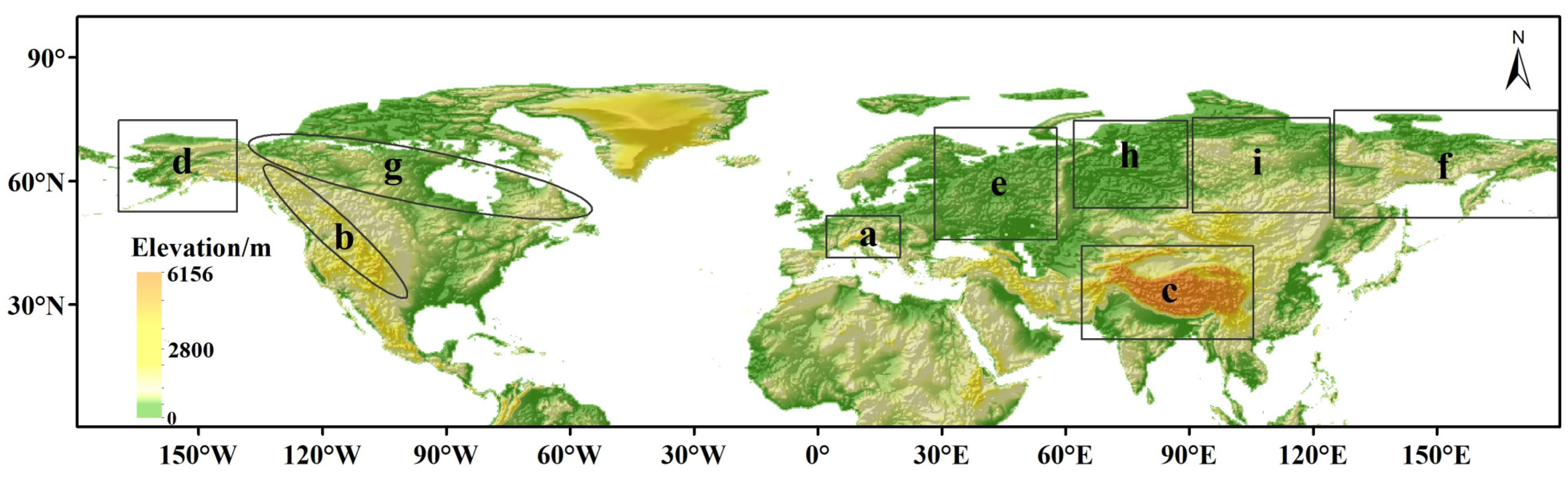
2.1. Study Area

Earth’s three poles, the Arctic, the Antarctic, and the Qinghai–Tibet Plateau, are susceptible to the climate change. Systematic research incorporating the three poles plays a critical role in studying global changes [19]. Therefore, based on the characteristics of high latitude or high altitude in the polar regions, we analyzed the spatio-temporal variability in terms of snow cover in the NH and nine typical areas located at high latitudes or high altitudes. The typical areas in the NH are shown in Figure 1, including six high latitudes and three high altitudes.
The high altitudes include the Alps, the Rocky Mountains, and the Qinghai–Tibet Plateau. The Alps is located in Europe, covering many countries, with an average elevation of 3000 m. The Rocky Mountains run through Canada and the western United States and are an important watershed for the North American climate, generally at an elevation of 2000 to 3000 m. The Qinghai–Tibet Plateau is located in southwest China and is called the third pole in the world, with an average elevation of 4000 m and an extreme climate. Moreover, a very complex orography characterizes these areas, with large elevation gradients and deep valleys of different orientations intersecting the ridge and shaping numerous mountain massifs [46]. The high latitudes include Alaska, the Eastern Europe Plain, the Eastern Siberia Mountains, Northern Canada, the Western Siberia Plain, and the Central Siberian Plateau. These areas are located in the north of North America and Eurasia, and most areas within of them are characterized by a latitude greater than 60°N. Therefore, we can assume that these high latitudes share some of the characteristics of the Arctic.
When analyzing changes in SP, to avoid the influence of instantaneous snow-covered areas, areas with snow-cover days larger than ten days were considered based on the average annual SCD over the NH. In addition, the Arctic Archipelago was excluded from this study.

2.2. NHSD and GlobSnow Datasets

This analysis was conducted based on a long time series of daily snow depth over the Northern Hemisphere (NHSD) and the Global Snow Monitoring for Climate Research (GlobSnow) V3.0 dataset. Both GlobSnow V3.0 and NHSD are passive microwave remote sensing products that use the brightness temperature data from the SMMR, SSMI, and SSMIS sensors archived in the National Snow and Ice Data Center (NSIDC). GlobSnow V3.0 is available from the European Space Agency (ESA, http://www.globsnow.info/swe/, accessed on 9 October 2021); this dataset covers areas between 35°N and 85°N and the period from 1979 to 2018 at a spatial resolution of 25 km. An assimilation algorithm was adopted in GlobSnow V3.0 [47,48] to obtain the optimized snow particle size by the combining snow microwave radiation transmission model (HUT) and in situ SD data to enhance the SD estimation accuracy. GlobSnow has been reported to be the most accurate SD dataset in the world [40,41,42]. Unfortunately, GlobSnow V3.0 is unavailable for mountainous regions and regions south of 35°N.
The NHSD dataset is provided by the National Tibetan Plateau Data Center (TPDC, https://poles.tpdc.ac.cn/, accessed on 9 October 2021) and covers the period from 1980 to 2018. This dataset was produced based on passive microwave brightness temperatures obtained from three sensors (SMMR, SMM/I, and SMMI/S) using a modified Chang algorithm [49,50]. During the NHSD process, the brightness temperatures of these different sensors were cross-calibrated to enhance the temporal consistency of this dataset [51]. Then, the relationship between the in-situ SD and brightness temperature difference between 18 and 36 GHz was established each month at each station pixel to obtain regression coefficients corresponding to each station. These station-specific monthly coefficients were then interpolated to the regional scale to obtain the dynamic algorithm. In forested areas, the forest cover fraction derived from the global land cover map [52] was used to reduce the influence of forests. The NHSD dataset was validated using station data, showing that the relative bias of the global snow depth data is within 30%. Additionally, the high accuracy of the NHSD dataset in mountainous areas was clarified by Xiao [53]. The pixel size of the NHSD dataset is 0.25°, and the projection coordinate system is WGS84; this dataset covers the whole NH mainland.
This study considered the 1988 to 2018 period covered by the two snow depth datasets. The NHSD dataset was used to analyze SD in mountainous areas and the SP across the NH. The SD analyses in non-mountainous areas of the NH were conducted based on the GlobSnow V3.0 dataset.

2.3. Auxiliary Datasets

2.3.1. Ground Observation Datasets

Passive microwave datasets are frequently used for SD retrievals and monitoring but have rarely been used for SP detections in previous studies. In this study, we validated the snow phenology information retrieved from the NHSD dataset using three globally available ground observation datasets, including the Global Historical Climatology Network-Daily (GHCN-Daily) dataset and meteorological observation data recorded in China and the former Soviet Union. The GHCN-Daily dataset is a comprehensive database, the newest version of which comprises climate data from many sites and institutions in more than 180 countries around the world [54] (https://doi.org/10.7289/V5D21VHZ, accessed on 20 October 2021). A total of 15706 sites in that database recorded SD from 1988 to 2018. Snow depth data of China was provided by the China National Meteorological Administration (http://data.cma.cn/, accessed on 20 October 2021); we collected snow depth data from 923 meteorological stations over the period of 1988–2018. The third kind of snow depth observation data published by the Russian meteorological center (http://aisori.meteo.ru/, accessed on 20 October 2021) was recorded at 613 stations from 1988 to 2018.
Due to the different sources of ground observation datasets, the quality and quantity of data corresponding to each site differed. To minimize random and systematic errors in the ground observation datasets and accurately retrieve SP information, it was essential to operate a quality control from 1988 to 2018. The methods used to screen the ground observation datasets are described as follows:
(1)
Quantity of data: if the quantity of data corresponding to a certain site in the study period was greater than or equal to 90% of the total data, these data were retained.
(2)
Distribution of data: data may have been unevenly distributed in certain years following step (1). Here, the data obtained in a given year at a certain site were divided into five-day groups, resulting in a total of 73 data groups; then, a judgment was made. If the number of valid values corresponding to each group was greater than or equal to four, the site was retained.
After the above two screening steps were performed, a total of 1797 sites in nine typical areas were retained and the SP information of these sites was obtained. Unfortunately, we found few matching sites in the Alps and the Qinghai–Tibet Plateau when the snow phenology information extracted from the two datasets was matched at the pixel scale and time series. This may have been caused by the large amount of transient snow cover that exists in the relatively low-latitude Alps and Qinghai–Tibet Plateau and the strict SP parameter definition (described in Section 3.2) adopted in this study. Hence, a comparative snow cover phenology analysis could not be conducted between the NHSD dataset and ground observation datasets in the Alps and the Qinghai–Tibet Plateau. Finally, a total of 496 sites in seven typical areas were reserved (Table 1), and we took seven typical areas as representative areas to study the feasibility of monitoring SP using the NHSD passive microwave snow depth dataset in Section 5.1.

2.3.2. IMS and ERA Datasets

The Interactive Multi-Sensor Snow and Ice Mapping System (IMS) [55,56] is manufactured by the United States National Ice Center (USNIC). The IMS dataset combines multiple optical and microwave sensors to provide coverage of snow, lake ice, and sea ice in the NH, free from cloud disturbance. This dataset provides daily snow and sea ice information collected from February 1997 to the present and has undergone several version updates since its release. Limited by the timespan length and the large scale of the study area considered in this study, the IMS dataset version with a 24 km spatial resolution was considered over the timespan from 1998 to 2019. The IMS dataset was used to extract SP information that was then compared to the SP derived from the NHSD dataset.
The ERA-Interim dataset [57] is provided by the European Centre for Medium-Range Weather Forecasts (ECMWF); this dataset is available from 1979 to 2019 (https://apps.ecmwf.int/datasets/data/interim-full-daily/, accessed on 20 July 2021). The snow parameters of ERA-Interim are derived from the Tiled ECMWF Scheme for Surface Exchanges over Land (TESSEL). The SWE and snow density information derived from 1980 to 2016 were employed in this study. The SD data of ERA-Interim were obtained by dividing the SWE by the snow density. The SP information was also derived from the ERA-Interim snow depth data and compared to that obtained from the NHSD dataset.

3. Methods

3.1. GlobSnow and NHSD Datasets Preprocessing

In this study, a complete snow hydrological year was defined as the period lasting from 1st September to 31st August the following year. Therefore, the study period (1988–2018) corresponded to 30 snow hydrological years. We analyzed the spatio-temporal variations in SD only from October to May due to data scarcity in the GlobSnow dataset from June to September. Because the projection and data types of GlobSnow and NHSD are different, we used the NHSD dataset as the standard for adjustment. We converted the GlobSnow projection to WGS84 and divided the SWE values in GlobSnow by the snow density (0.24 g/cm3) to obtain the SD.
However, some gaps in the study period (from October to May) remained in the GlobSnow daily SD dataset. To derive the monthly and yearly SD, we performed special preprocessing. First, the daily SD in a certain month were divided into six groups at the pixel scale; then, we judged whether the number of valid SD values in each group was larger than or equal to three (if the sixth group had fewer than five days, the judgment threshold was set to two). If the number of valid SD values was greater than or equal to three, the mean SD value of the group was calculated; otherwise, the mean SD value of the group was considered an invalid value. Next, the number of mean SD values obtained in the previous step was calculated. If this number was larger than or equal to four, the mean SD value of the valid values was calculated and used as the monthly average SD; otherwise, the value was regarded as invalid. Likewise, the mean SD value of the valid values was calculated and regarded as the annual SD of the snow hydrological year if the number of valid monthly average SD values was greater than or equal to seven; otherwise, the value was regarded as invalid.

3.2. Definition of Snow Phenology

The SP parameters derived from the NHSD dataset, including the SCOD, SCED, SD, and SCD, were defined as follows:
(1)
An SD greater than or equal to 3 cm was considered snow cover.
(2)
The first day on which the SD was greater than or equal to 3 cm and the length of continuous snow cover exceeded five days in the snow hydrological year was considered the snow cover onset day (SCOD).
(3)
The last day on which the SD was greater than or equal to 3 cm and the length of continuous coverage exceeded five days in the snow hydrological year was considered the snow cover end day (SCED).
(4)
The difference between the SCED and SCOD was regarded as the number for the snow season length (SSL).
(5)
The number of days with an SD greater than or equal to 3 cm on a given pixel in the snow hydrological year was considered the snow cover duration (SCD).
The five-day continuous snow cover setting in the definition of the SCOD and SCED effectively avoided the influence of instantaneous snow cover in autumn and spring on the extracted SCOD and SCED values [20]. The criteria used to establish snow or no snow differ among the diverse datasets employed in this study and are described as follows:
(1)
For the passive microwave dataset NHSD, the snow cover threshold is 3 cm due to uncertainties regarding shallow and thin snow measurements when using passive microwave snow cover inversion methods [58].
(2)
The model-simulation ERA-Interim dataset considers an area to be snow-covered when the snow depth is greater than 0 cm.
(3)
In the IMS dataset, pixel values of 4 or 165 are considered to be snow-covered [55].
(4)
The SD criterion for the ground observation datasets is 0.5 cm.

4. Results

4.1. Changes in Snow Depth

The results of the analysis of spatial variations in annual average SD in the NH are shown in Figure 2. Negative SD trends were found in most areas of the NH during the 1988–2018 period. These areas of decreasing SD were mainly distributed in Alaska, the north of the Rocky Mountains, Canada, the Scandinavian Peninsula, the Eastern European Plain, the West Siberian Plain, the Central Siberian Plateau, Central Asia, Mongolia, and China. Among them, the SD in many areas showed slight declining trends, with change rates between −0.5 cm/a and −0.01 cm/a. In a few fragmentary areas, the SD reduction rates reached values between −1.5 cm/a and −0.5 cm/a, passing the significance test at the 0.05 significance level. In contrast, the SD showed positive trends in northern Mongolia, central Northeast China, and in some mountainous regions of the Qinghai–Tibet Plateau, with smaller change rates varying between 0.01 cm/a and 0.5 cm/a. Higher SD growth rates were found in western Northwest Canada, scattered areas of the central and southern Rocky Mountains, and a number of areas in the Eastern Siberia Mountains; these growth rates ranged from 0.5 cm/a to 1 cm/a. In particular, the SD showed significant increasing trends in the southern Rocky Mountains and the Eastern Siberian Mountains.
The results of the analysis of interannual variations in monthly average SD from 1988 to 2018 are illustrated in Figure 3 and Figure 4. From November to March, the SD declined slightly in most of the high latitudes of North America, with rates ranging from −0.5 cm/a to −0.01 cm/a, with higher rates ranging from −2.5 cm/a to −1.5 cm/a (significant declines) being identified in some specific fragmented areas. This was also the case in the Eastern European Plain from November to January. The SD in the Western Siberian Plain and the Central Siberian Plateau from November to April was highly spatially heterogeneous: positive changes were intermixed with negative changes. However, the SD in May presented a significant decrease across the Central Siberian Plateau. The SD in the Eastern Siberia Mountains (except for Kamchatka) exhibited a positive trend in all months, especially from December to April.
Among high altitudes, the SD decreased in the northern Rocky Mountains and increased in the central and southern Rocky Mountains from October to February. The SD in most areas of the Alps showed significant increasing trends (with rates ranging from 0.01 cm/a to 0.5 cm/a), while opposite trends were observed throughout the area in May, with small decreasing rates. The SD in the Qinghai–Tibet Plateau was spatially heterogeneous, increasing significantly in the northern mountains and decreasing in most of the central areas from October to May. The Nyingchi Tanggula Mountains in the southeastern Qinghai–Tibet Plateau, which always has deep SD, showed a clear downward trend in SD from December to January. Although the spatial change pattern observed in the Qinghai–Tibet Plateau was complex, the rates of change were small and similar to those indicated in the Alps.
The SD in the NH generally presented a significant decreasing trend (p < 0.01), with a rate of −0.055 cm/a during the 1988–2018 period (Figure 5). Before 2010, the SD in the NH showed a strongly significant decreasing trend (p < 0.01), with a rate of −0.065 cm/a. In contrast, since 2010, the SD showed a significant increasing trend (p < 0.05), with a rate of 0.139 cm/a. In particular, continuously increasing SD trends were found in 2016/2017 and 2017/2018. In this study, the minimum SD (8.2cm) in the NH occurred in 2010.

4.2. Changes in Snow Phenology

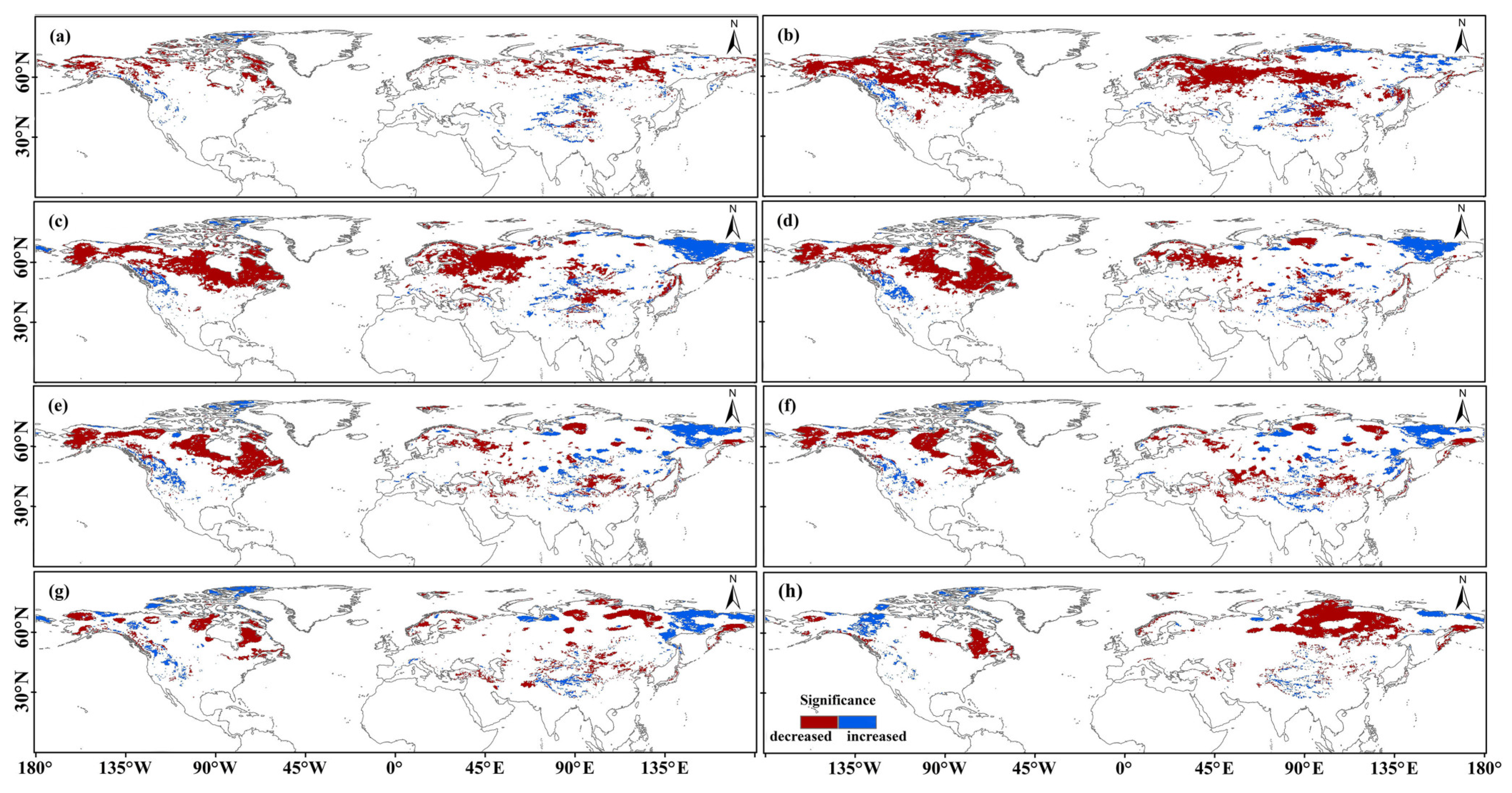
4.2.1. Spatial Distributions of SCOD, SCED, SSL and SCD

The spatial distribution patterns for the annual average SP from 1988 to 2018 are reported in Figure 6. The SP presented both latitudinal and vertical zonal distributions; in detail, the higher the latitudes and altitudes were, the earlier the SCOD occurred, the later the SCED occurred, and the longer the SCD and SSL were. Across the NH, areas where the SCOD occurred in December (on days 91–120) accounted for the largest proportion of the NH, at 15.5%; these areas were mainly located at middle and high latitudes. The earliest SCOD occurred in northern Alaska, the western Karakoram Mountains, and the western Himalayas in September (on days 1–30). The snow cover distributed in most areas between 30°N and 45°N ended in February (on days 150–180). Areas in which snow cover ended in May (on days 241–270) accounted for the largest proportion of the NH mainland, at 16.8%; these areas were mainly concentrated at high latitudes. The snow cover in 14.3% of the NH (mainly in the Arctic region, parts of the Rocky Mountains, and the Qinghai–Tibet Plateau) disappeared after May.
The SSL and SCD presented similar spatial distribution characteristics in most areas of the NH (Figure 6). The highest SCD and SSL, with values corresponding to periods longer than nine months, were found in the Pamirs, western Karakoram Mountains, and western Himalayas. The SCD and SSL were between seven and nine months in some areas of the Arctic and the western Qinghai–Tibet Plateau. By comparing the spatial distribution characteristics of the SSL and SCD, we found that proportions of areas corresponding to time periods from 10 to 60 days exhibited the greatest differences. Areas with an SSL between 10 and 60 days accounted for 6.5% of the NH, while areas with SCD between 10 and 60 days accounted for 10.2% of the NH. In this case, we found that the areas exhibiting differences were mainly located between 30°N and 45°N and were characterized by the widespread occurrence of transient snow cover due to the relatively low latitudes and high temperatures.

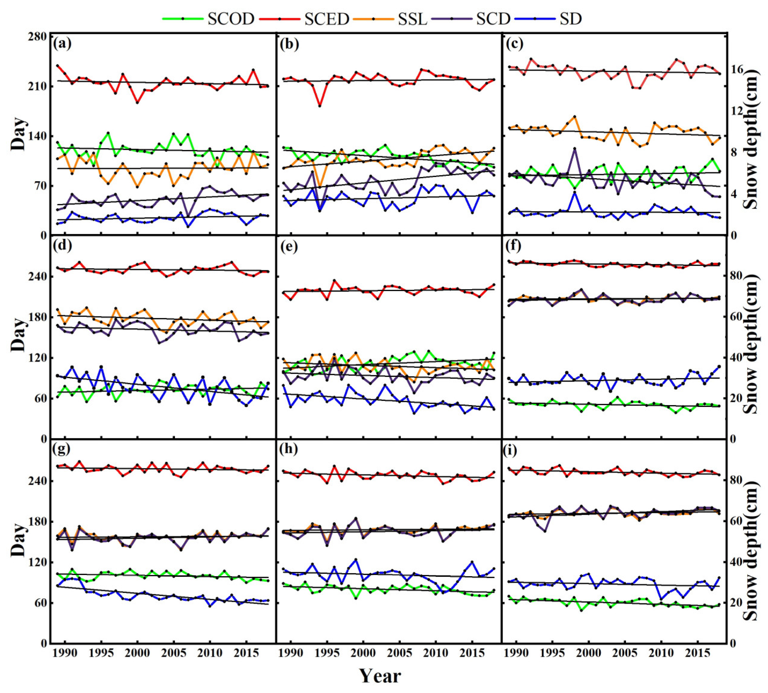
4.2.2. Interannual Variations in SCOD, SCED, SSL, and SCD

The interannual variations in SCOD, SCED, SSL, and SCD from 1988 to 2018 are shown in Figure 7 and Figure 8. In North America, areas with delayed SODs were mainly located in large parts of Alaska and Northern Canada, but the delay rates were small in these areas. In contrast, the SCOD advanced in the western mountains of the United States, and significantly advanced in fragmented areas (with rates more than two days/a). In Eurasia, the SCOD was delayed in most areas of Scandinavia and the Eastern European Plain, with relatively high delay rates of one–two days/a, especially in large parts of the Eastern European Plain. In the Siberia, the SCOD in most areas presented positive patterns. The spatial distribution of the SCOD in the Qinghai–Tibet Plateau was heterogeneous; in detail, the SCOD in the northern Qinghai–Tibet Plateau was significantly advanced, while the western and southeastern Tanggula Mountains and Nianqing Tanggula Mountains experienced significantly delayed SCODs. In other regions of the Qinghai–Tibet Plateau, negative patterns were intermixed with positive ones. According to the statistics, 60% of the NH had relatively small interannual SCOD variation slopes, within 0.5 days per year. More areas experienced SCOD advances (31.57%) than SCOD delays (21.10%), and more areas in the NH exhibited significantly advanced SCODs (5.90%) than significantly delayed SCODs (2.72%).
Across the NH, the SCED was delayed significantly in the central and southern Rockies of North America, with delays of one–two days per year recorded in some fragmented areas. This trend was also observed in Western Europe and northeast China, but the delay rates were smaller than those observed in the former region. In contrast, in most of the West Siberian Plain and the Central Siberian Plateau, the SCED showed significant advancing trends, especially in the Arctic region, where the SCED advanced by 0.5 to 1 days/a. The SCED across most of the Qinghai–Tibet Plateau showed significant advancing trends, advancing more than two days/a in some specific areas. According to the statistics, the SCED in 76.35% of the NH had relatively small interannual variation slopes, within 0.5 days per year, and more areas in the NH experienced advanced SCEDs (37.29%) than delayed SCEDs (14.77%).
The SCD and SSL displayed consistent spatial variation patterns in most areas of the NH. In North America, the SCD and SSL in most areas of Alaska, the Northwest Territories of Canada, Hudson Bay, and the Labrador Plateau showed negative trends. However, the SCD and SSL increased significantly in the Central Mountains of North America, increasing by more than two days/a in a few fragmented areas. In Eurasia, the SSL and SCD showed negative trends in Eastern Europe and positive trends in Central Europe. In the Qinghai–Tibet Plateau, the SSL and SCD decreased in most areas but increased in northern mountainous regions such as the western Kunlun Mountains and Altun Mountains. Comparing the changes in SCD and SSL, only in some fragmented areas, such as in parts of the central United States, did the SSL show decreasing trends while the SCD showed slight increasing trends. According to the statistics, approximately 60% of the NH experienced small interannual variation slopes in terms of SCD and SSL, within 0.5 days per year; fewer areas in the NH experienced SCD decreases (21.60%) than SD decreases (26.89%).

4.3. Characteristics of Snow Depth and Phenology in Typical Areas

A macro-comparative analysis of the SD and SP characteristics (SCOD, SCED, SCD, SSL) at high latitudes and high altitudes was carried out in this study. The results are reported in Table 2 and Figure 9.
The interannual variations in SD among the nine typical areas (Figure 9) showed that, for high altitudes, the SD in the Alps and the Rocky Mountains presented slight increasing trends, with growth rates of 0.013 cm/a and 0.018 cm/a, respectively. In the Qinghai–Tibet Plateau, the SD insignificantly decreased, with a slope of −0.003 cm/a. At high latitudes, specifically of Alaska, the Eastern European Plain, Northern Canada, the West Siberian Plain, and the Central Siberian Plateau, the SD showed negative trends, whereas the SD in the Eastern Siberian Mountains showed a positive trend. The SD in Northern Canada, Alaska, and the Eastern European Plain decreased significantly (p < 0.01), with slopes of −0.300 cm/a, 0.348 cm/a, and 0.230 cm/a, respectively. The SD in the Eastern Siberian Mountains showed a slight upward trend (with a slope of 0.076 cm/a).
With regard to the SCOD, at high altitudes, the advancing rate in the Rocky Mountains was the greatest, at 0.678 days per year, passing the significance test at the 0.01 level. The SCOD in the Alps also advanced, but this trend was insignificant. In contrast to these two areas, the SCOD in the Qinghai–Tibet Plateau showed an insignificantly delayed trend, with a rate of 0.156 day/a. At high latitudes, the SCOD in the Eastern Siberian Mountains, Northern Canada, the West Siberian Plain, and the Central Siberian Plateau was advanced. Among these areas, the SCOD in the West Siberian Plain and Central Siberian Plateau advanced significantly, especially in the Central Siberian Plateau, where the SODs advanced by 0.346 days per year, passing the significance test at the 0.01 level. The SCOD was delayed in Alaska and the Eastern European Plain; in the latter region, the SCOD was significantly delayed (p < 0.05) by 0.466 days per year.
Of the nine typical areas analyzed in this study, the SCED was insignificantly delayed in the Rocky Mountains and Eastern European Plain. Negative SCED trends were found in the remaining seven typical areas; in particular, significant advancing trends (p < 0.05) occurred in the Eastern Siberian Mountains and the Central Siberian Plateau, where the SCED occurred 0.135 and 0.215 days per year earlier, respectively.
The SCD and SSL trends were consistent in each typical area. The SCD and SSL increased in the Alps and the Rocky Mountains, the Eastern Siberian Mountains, Northern Canada, the West Siberian Plain, and the Central Siberian Plateau. Specifically, in the Rocky Mountains, the SSL and SCD growth rates were 0.78 days/a and 0.95 days/a, respectively, both of which passed the significance test at the 0.01 level. The SSL and SCD decreased in the Qinghai–Tibet Plateau, Alaska, and the Eastern European Plain; the decrease slope for SCD in the Qinghai–Tibet Plateau was significant.
The comprehensive comparative results of these snow parameters among the nine typical areas are summarized as follows:
(1)
Most typical areas were characterized by decreased SD, advanced SCOD and SCED, and insignificantly increased SCD and SSL trends.
(2)
The SCD and SSL were similar at high latitudes. The SSL was larger than the SCD at high altitudes; this may have been related to the presence of extensive transient snow cover in relatively low-elevation regions.
(3)
The general trends in SD, SSL, and SCD were consistent at high altitudes, while the trends in SSL and SCD at high latitudes were consistent. The interannual SD, SSL, and SCD fluctuations were similar in each typical area.
(4)
The SCOD variations influenced the changes in SCD and SSL. The SCD and SSL increased with an advanced SCOD and SCD, and the SSL decreased with a delayed SCOD.

5. Discussion

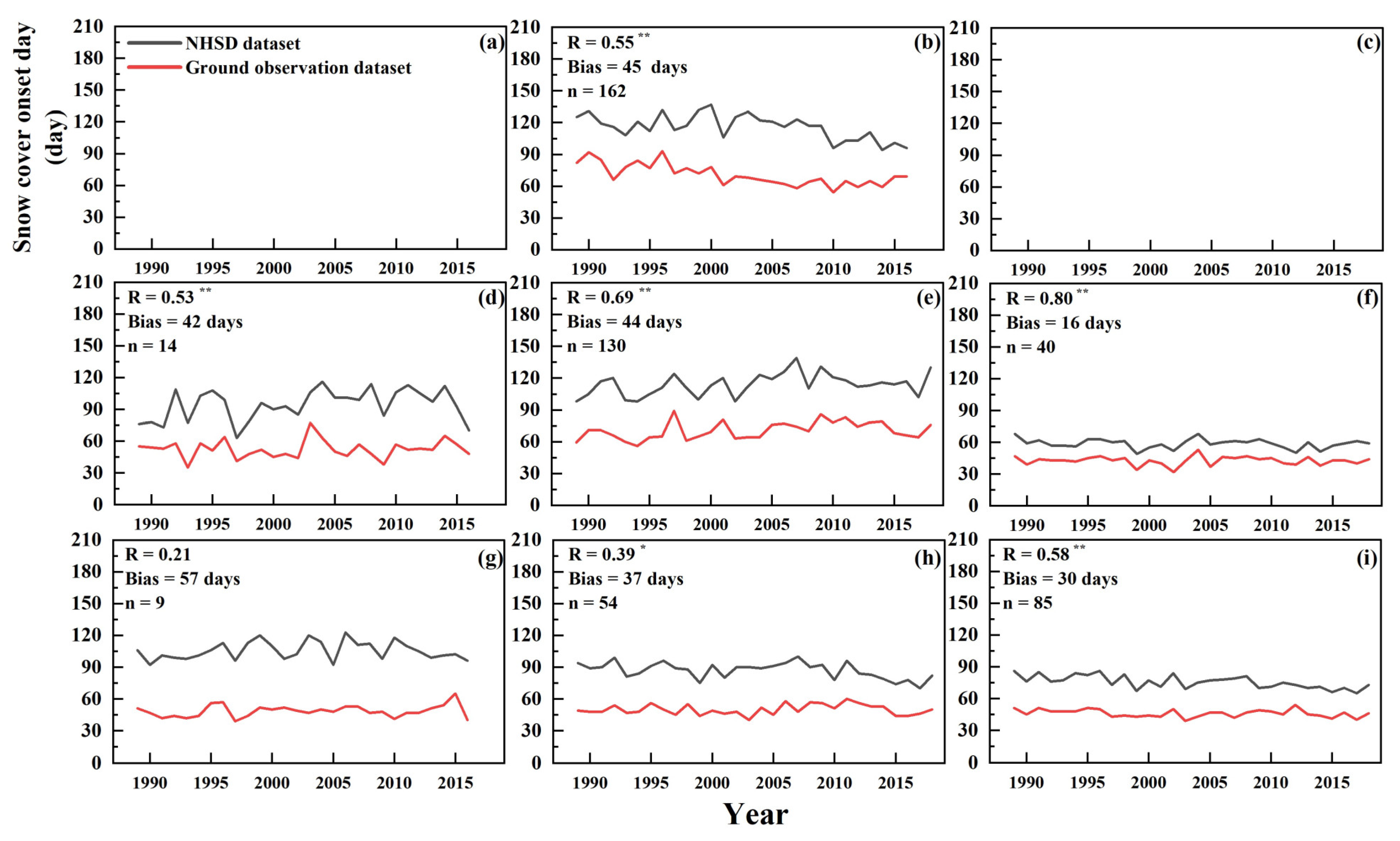
5.1. Comparisons with Ground Observation Datasets

The passive microwave snow depth dataset NHSD has never been used for SP information extraction before. Although Zhu [45] used the WESTDC, a Chinese passive microwave snow depth data source with the same algorithm as NHSD, to extract and analyze SP in China, she did not assess the accuracy of the SP information. To assess the accuracy of the SP information, we compared the SP information obtained from the NHSD dataset with that obtained from ground observation datasets in seven typical areas. The correlation coefficient (R) and bias values were employed to express the comparison results derived in this study.
The SCOD trends extracted from the NHSD dataset were consistent with that derived from the ground observation datasets in most areas (Figure 10), such as in the Rocky Mountains, Alaska, the Eastern European Plain, the Eastern Siberian Mountains, and the Central Siberian Plateau. The R values derived between these datasets were greater than 0.5 and passed the significance test at the 0.01 level. The R value obtained in Northern Canada performed badly, which may have been related to the small sample size (n = 9) applied in this study. Although the SCOD trends were consistent between the NHSD and ground observation datasets, there were also some differences in these values. The largest differences occurred in Northern Canada (bias = 57 days), and relatively small differences occurred in the Rocky Mountains, Alaska, the Eastern European Plain, the West Siberian Plain, and the Central Siberian Plateau, with an average bias of 40 days. The bias in the Eastern Siberian Mountains was the smallest, at 16 days. Moreover, we found that the ground observation datasets detected snow cover earlier than the NHSD dataset in the seven typical areas.
The SCED comparison results shown in Figure 11 indicated a strongly significant correlation between the NHSD and ground observation datasets in the Eastern European Plain, the West Siberian Plain, and the Central Siberian Plateau, with R values greater than 0.7, passing the significance test at the 0.01 level. In addition, the R values in the Rocky Mountains, Alaska, the East Siberian Mountains, and Northern Canada were also greater than or equal to 0.46, passing the significance test at the 0.05 or 0.01 level. It is important to note that not only were the SCED trends observed between the NHSD and ground observation datasets consistent, the average bias between these datasets in the seven areas was only approximately −2 days. As a result, the NHSD dataset can be said to be credible and critical for detecting and estimating the SCED in large-scale areas.
The SSL consistency between the NHSD and ground observation datasets was subject to the SCOD and SCED. As a result, the R values derived from these datasets exhibited good performances except in Northern Canada. The SCD consistency between the NHSD and ground observation datasets was well documented and shown in Figure A2. The R values for the SCD derived between the two datasets were larger in most areas than the R values for the SSL, indirectly demonstrating the accuracy of the NHSD dataset. With regard to the SSL and SCD, the values extracted from the NHSD dataset were lower than those observed on the ground. The biases between the SSL and SCD were similar in each typical area. Specific diagrams are shown in Figure A1 and Figure A2 in Appendix A.
In summary, the observed change trends in SP information (SCOD, SCED, SSL, and SCD) obtained from the NHSD dataset were similar to those derived from the ground observation datasets, especially the SCED trends (for which relatively high correlations and low biases were obtained). Relatively large biases arose when detecting the SCOD; these biases may have been related to the SP definition applied in this study (an SD greater than or equal to 3 cm was considered snow cover) or to the insensitivity of passive microwave brightness temperatures when detecting less and shallow snow [58]. A third reason could be the scale dependency of the ground observations [59,60]. Although relatively large biases occurred in some snow parameters, the general trends described by the two datasets were consistent, and the derived interannual fluctuations presented similar characteristics that did not affect the usage of the NHSD dataset in the trend analysis. As a result, large-scale SP information can be effectively detected using the NHSD dataset to reflect the spatio-temporal characteristics of snow phenology in the NH, thus overcoming the limitations associated with phenological monitoring with traditional ground observations and optical remote sensing data.

5.2. Comparisons with the IMS and ERA-Interim Datasets

To further analyze the accuracy of the SP information, we also compared SP information obtained from the NHSD dataset with that derived from the IMS and ERA-Interim datasets in the nine typical areas during the overlapping time period (1999–2016); the comparative results are shown in Figure 12, Figure 13, Figure A3 and Figure A4. For all typical areas, the appearance (disappearance) of snow cover was the first (last) detected by ERA-Interim. By contrast, the NHSD dataset was the last (first) to indicate the appearance (disappearance) of snow cover. The difference may be largely related to the SP definition applied in this study (an SD greater than or equal to 3 cm was considered as snow cover for NHSD, while for ERA-Interim, an SD greater than or equal to 0 cm was considered as snow cover).
Among the high altitudes, the SCOD derived from the IMS and ERA-Interim datasets presented consistency in the Alps and the Rocky Mountains. Although the NHSD dataset showed the opposite trend to the above two datasets, it showed similar interannual fluctuations over many years. In the Qinghai–Tibet Plateau, a high degree of agreement was demonstrated between the NHSD and IMS datasets when detecting the SCOD, both in terms of the SCOD values and trends. The ERA-Interim dataset performed differently from the other two datasets in the Qinghai–Tibet Plateau. For high latitudes, the SCOD obtained from the NHSD and IMS datasets presented consistent trends in almost all typical areas. The ERA-Interim dataset appeared to be inconsistent with the other two datasets in some areas, which might have been related to the inaccuracy of the model data itself [61,62].
The SCED derived from the three datasets showed identical trends at high latitudes, which may be related to the physical characteristics of relatively high snow densities and strong scattering during the snow termination period as well as high temperatures, lead to rapid snow melt, which facilitates less intrusive and simpler remote sensing monitoring. The SCED values extracted from the NHSD and IMS datasets were similar, while those obtained from the ERA-Interim dataset differed, especially at high altitudes.
The SSL obtained from the NHSD, IMS, and ERA-Interim datasets showed identical decreasing trends among high latitudes (except in the Eastern Siberian Mountains) (Figure A3 in the Appendix A). For the SCD, the same general trend was detected by all three datasets in the Qinghai–Tibet Plateau. However, the interannual fluctuations of the NHSD were different from the other datasets in most of years. In this case, it is hard to say which extracted phenology is more accurate because of the lack of comparable results from the ground observation datasets in Section 5.1. In contract to the Qinghai–Tibet Plateau, although the overall trends in the Alps and the Rocky Mountains were different, the interannual fluctuation was very similar. The SCD trends from the IMS dataset were consistent with those from the ERA-Interim dataset in the Alps and Rocky Mountains, but similar interannual fluctuations were found in the three datasets. Combining the results of the comparisons with the ground-based observations in Section 5.1, we can confirm that IMS and ERA-Interim underestimated the SCD in the Rocky Mountains after the year 2000, which is mainly due to IMS’s lack of ability of to recognize strong snow storms on cloudy days [63] and the inaccuracy of the model data itself [61,62]. At high latitudes, except for in Northern Canada, identical decreasing trends and similar values were obtained from the three datasets in five of the typical areas. Specific diagrams reflecting these comparisons are shown in Figure A4 in the Appendix A.
In summary, the comparison of SP information from NHSD with that from IMS and ERA-Interim has demonstrated a better correspondence of the datasets at high latitudes. At high altitudes, the performance of the three datasets is uncertain. The large bias in snow phenology detected by the ERA dataset is consistent with the results reported by Xiao [41] and may be related to the SP definition applied in this study (an SD greater than or equal to 0 cm was considered snow cover) or the inaccuracy of the model data itself [61,62].

5.3. Comparisons with Existing Studies

With regard to the SD in the NH, our finding of significantly decreasing SD trends is consistent with the results reported by Xiao [39] obtained in the corresponding period. The continuous increasing SD trends identified in 2016/2017 and 2017/2018 are consistent with the snow mass research results obtained by Pulliainen [40]. The latitudinal and vertical zonal spatial distributions patterns in regard to SP we report in this study are consistent with the results reported in [20,22,64].
We also compared the results of the study in terms of different areas with those of previous results in this section. In Europe, we reported delayed SCODs in the Eastern Europe Plain and the southeastern Qinghai–Tibet Plateau, similar to the results claimed by Zhong [22], who analyzed data recorded at meteorological stations across Eurasia from 1966 to 2012. However, our findings corresponding to the Eastern European Plain are in contrast to those of Sun [28], who claimed that the SCOD insignificantly advanced from 2000 to 2016. In the Qinghai–Tibet Plateau, we reported an insignificant decrease in SD, consistent with the results reported in [65]. The decreased SCD in the Qinghai–Tibet Plateau we reported from 1988 to 2018 are consistent with the results reported in Huang [66], Wang [33], Qiao [67], and Che [65], who found consistent results over the 1980–2015, 2001–2015, 2001–2014, and 1980–2009 periods, respectively. In the Alps, the observed increasing SD trend in winter is in contrast to some previous studies, while the decreased SD trend in May reported herein is consistent with the findings of previous studies [68,69,70,71]. The positive SCD trends reported in this study are inconsistent with the results found by Notarnicola [32] through MODIS data over the time period lasting from 2000 to 2018.
At the high latitudes of North America, we found that the monthly average SD decreased significantly in winter, consistent with the results reported by Jeong [43] in regard to interannual SWE variations from February to March. With regard to SP, the significantly advanced SCOD, delayed SCED, and significantly increased SSL observed herein in the central Rocky Mountains are consistent with the results of Chen [64] over the 2001–2020 period. Additionally, the notable SCED delay and SSL increase identified in the Rocky Mountains are similar to the results of Brown [72] derived from 1981 to 2017. The increasing SCD we observed in the central and southern Rocky Mountains are consistent with the results reported by Canada’s Changing Climate Report: seasonal snow accumulation increased by 2% to 5% per decade from 1981 to 2015 in southern Saskatchewan and parts of Alberta and British Columbia [23]. However, the results for the Rocky Mountains we report appear to contradict what Mote [24] reported: 33% of snow monitoring sites recorded significant decreasing trends, while only 2% of sites showed a significant increasing trend in the Rocky Mountains on 1 April from 2005 to 2018.
We summarized the possible reasons for the above differences as follows: (1) Differences in the applied study periods and trend calculation methods could cause different results. (2) The different datasets used in scientific research could cause different results. For example, the different results generated using ground observations and remote sensing data may be explained by the scale dependencies of the ground observations [59,60]. (3) The different SP definitions applied in different studies could also be an important source of discrepancies, especially discrepancies in the snow cover onset time.

6. Conclusions

In this study, we analyzed spatio-temporal variations in snow depth and snow phenology in the NH from 1988 to 2018 and conducted a macro-comparative analysis of the characteristics of snow depth and snow phenology in regard to the high latitudes and high altitudes. Our main findings are summarized as follows:
(1)
Snow depth in the NH showed a significant decreasing trend from 1988 to 2018, with a rate of −0.55 cm/decade. Different snow depth changes were observed between the pre-2010 period and the post-2010 period. Changes in snow depth were insignificant at high altitudes, while significant decreases were found at high latitudes.
(2)
The NHSD dataset was shown to be capable of obtaining large-scale and long-term snow phenology information via comparisons with ground observation datasets, IMS, and ERA-Interim. The snow phenology parameters presented both latitudinal and vertical zonal distributions; in detail, the higher the latitude and altitude was, the earlier the snow cover onset day occurred, the later the snow cover end day occurred, and the longer the snow cover duration and snow season length were. The areas associated with an earlier snow cover onset day were 10.47% larger than the delayed areas in the NH. The snow cover onset day occurred earlier at high altitudes except for the Qinghai–Tibet Plateau, as it did at most of the high latitudes. The areas associated with an advanced snow cover end day were 22.52% larger than the delayed areas in the NH. An advanced snow cover end day occurred in most typical areas.
(3)
Most typical areas were characterized by a decreased snow depth, an advanced snow cover onset day, an insignificantly advanced snow cover end day, and insignificant increasing trends in snow cover duration and snow season length. The snow cover duration and snow season length values were similar at high latitudes, while the snow season length value was larger than the snow cover duration value at high altitudes. The snow depth exhibited similar interannual fluctuation characteristics as snow cover duration and snow season length in each typical area. In addition, we found that the snow cover duration and snow season length increased and decreased corresponding to an advanced or delayed snow cover onset day.
In this study, we demonstrated the ability of the NHSD dataset to acquire large-scale and long-term snow phenology information and analyzed the characteristics of snow depth and snow phenology at high latitudes and high altitudes in the Northern Hemisphere from 1988 to 2018. However, the reasons for the similarities and differences in snow depth and phenology at high latitudes and high altitudes have not been explored in this study. In fact, snow cover in nature is a complex process, and changes in snow cover are influenced by a combination of long-term climate change conditions and short-term weather phenomena [40,73]. As a result, further work needs to consider both long-term monthly-to-seasonal climate conditions and short-term weather phenomena in order to accurately analyze and attribute phenomena identified at high latitudes and high altitudes with the help of physical models in order to strength our understanding of changes at the Earth’s three poles.

Author Contributions

Conceptualization, S.Y. and T.C.; methodology, S.Y. and L.D.; software, S.Y. and L.X.; formal analysis, S.Y. and J.D.; writing—original draft preparation, S.Y.; writing—review and editing, S.Y., T.C., L.D., L.X. and J.D. All authors have read and agreed to the published version of the manuscript.

Funding

This research was supported by the National Key Research and Development Program of China (2020YFA0608501), the National Nature Science Foundation of China (42125604, 42171143 and 42001289), the CAS ‘Light of West China’ Program (E029070101), and the China Postdoctoral Science Foundation (2022M713340).

Data Availability Statement

The GlobSnow SWE data are downloaded from ESA, NHSD snow depth datasets are provided by TPDC, and ERA-Interim and IMS are downloaded from ECMWF and NASA, respectively. The ground observation datasets are obtained from the meteorological administration from China, Russia and GHCN.

Acknowledgments

The authors thank the editors and anonymous reviewers for their constructive comments and suggestions for improving this paper.

Conflicts of Interest

The authors declare no conflict of interest.

Appendix A

Figure A1. Comparison of the SSL derived from NHSD and ground observation datasets in typical areas. The typical areas are (a) the Alps, (b) the Rocky Mountains, (c) the Qinghai–Tibet Plateau, (d) Alaska, (e) the Eastern European Plain, (f) the Eastern Siberian Mountains, (g) Northern Canada, (h) the West Siberian Plain, and (i) the Central Siberian Plateau. The vertical axis labels in panels (bi) are the same as those in panel (a). * and ** indicate that the correlation were significant at the 95% and 99% confidence level, respectively.
Remotesensing 14 05057 g0a1
Figure A2. Comparison of the SCD derived from NHSD and ground observation datasets in typical areas. The typical areas are (a) the Alps, (b) the Rocky Mountains, (c) the Qinghai–Tibet Plateau, (d) Alaska, (e) the Eastern European Plain, (f) the Eastern Siberian Mountains, (g) Northern Canada, (h) the West Siberian Plain, and (i) the Central Siberian Plateau. The vertical axis labels in panels (bi) are the same as those in panel (a). * and ** indicate that the correlation were significant at the 95% and 99% confidence level, respectively.
Remotesensing 14 05057 g0a2
Figure A3. Comparison of the SSL derived from NHSD, IMS, and ERA-Interim in typical areas. The typical areas are (a) the Alps, (b) the Rocky Mountains, (c) the Qinghai–Tibet Plateau, (d) Alaska, (e) the Eastern European Plain, (f) the Eastern Siberian Mountains, (g) Northern Canada, (h) the West Siberian Plain, and (i) the Central Siberian Plateau.
Remotesensing 14 05057 g0a3
Figure A4. Comparison of the SCD derived from NHSD, IMS, and ERA-Interim in typical areas. The typical areas are (a) the Alps, (b) the Rocky Mountains, (c) the Qinghai–Tibet Plateau, (d) Alaska, (e) the Eastern European Plain, (f) the Eastern Siberian Mountains, (g) Northern Canada, (h) the West Siberian Plain, and (i) the Central Siberian Plateau.
Remotesensing 14 05057 g0a4

References

  1. Bormann, K.J.; Brown, R.D.; Derksen, C.; Painter, T.H. Estimating snow-cover trends from space. Nat. Clim. Change 2018, 8, 923–927. [Google Scholar] [CrossRef]
  2. Flanner, M.G.; Shell, K.M.; Barlage, M.; Perovich, D.K.; Tschudi, M.A. Radiative forcing and albedo feedback from the Northern Hemisphere cryosphere between 1979 and 2008. Nat. Geosci. 2011, 4, 151–155. [Google Scholar] [CrossRef]
  3. Immerzeel, W.W.; van Beek, L.P.H.; Bierkens, M.F.P. Climate Change Will Affect the Asian Water Towers. Science 2010, 328, 1382–1385. [Google Scholar] [CrossRef] [PubMed]
  4. Barnett, T.P.; Adam, J.C.; Lettenmaier, D.P. Potential impacts of a warming climate on water availability in snow-dominated regions. Nature 2005, 438, 303–309. [Google Scholar] [CrossRef]
  5. Déry, S.J.; Brown, R.D. Recent Northern Hemisphere snow cover extent trends and implications for the snow-albedo feedback. Geophys. Res. Lett. 2007, 34, 2–7. [Google Scholar] [CrossRef]
  6. Sturm, M.; Goldstein, M.A.; Parr, C. Water and life from snow: A trillion dollar science question. Water Resour. Res. 2017, 53, 3534–3544. [Google Scholar] [CrossRef]
  7. Fugazza, D.; Manara, V.; Senese, A.; Diolaiuti, G.; Maugeri, M. Snow Cover Variability in the Greater Alpine Region in the MODIS Era (2000–2019). Remote Sens. 2021, 13, 2945. [Google Scholar] [CrossRef]
  8. Deng, J.; Che, T.; Xiao, C.; Wang, S.; Dai, L.; Meerzhan, A. Suitability analysis of ski areas in China: An integrated study based on natural and socioeconomic conditions. Cryosphere 2019, 13, 2149–2167. [Google Scholar] [CrossRef] [Green Version]
  9. Silberman, J.A.; Rees, P.W. Reinventing mountain settlements: A GIS model for identifying possible ski towns in the US Rocky Mountains. Appl. Geogr. 2010, 30, 36–49. [Google Scholar] [CrossRef]
  10. Lin, Y.; Jiang, M. Maximum temperature drove snow cover expansion from the Arctic, 2000–2008. Sci. Rep. 2017, 7, 15090. [Google Scholar] [CrossRef]
  11. Ke, C.; Li, X.; Xie, H.; Ma, D.; Liu, X.; Kou, C. Variability in snow cover phenology in China from 1952 to 2010. Hydrol. Earth Syst. Sci. 2016, 20, 755–770. [Google Scholar] [CrossRef] [Green Version]
  12. Liston, G.E.; Hiemstra, C.A. The Changing Cryosphere: Pan-Arctic Snow Trends (1979–2009). J. Clim. 2011, 24, 5691–5712. [Google Scholar] [CrossRef]
  13. Brown, R.D.; Robinson, D.A. Northern Hemisphere spring snow cover variability and change over 1922-2010 including an assessment of uncertainty. Cryosphere 2011, 5, 219–229. [Google Scholar] [CrossRef] [Green Version]
  14. Smith, N.V.; Saatchi, S.S.; Randerson, J.T. Trends in high northern latitude soil freeze and thaw cycles from 1988 to 2002. J. Geophys. Res. Atmos. 2004, 109, 1–14. [Google Scholar] [CrossRef] [Green Version]
  15. Pepin, N.; Bradley, R.S.; Diaz, H.F.; Baraer, M.; Caceres, E.B.; Forsythe, N.; Fowler, H.; Greenwood, G.; Hashmi, M.Z.; Liu, X.D.; et al. Elevation-dependent warming in mountain regions of the world. Nat. Clim. Change 2015, 5, 424–430. [Google Scholar] [CrossRef] [Green Version]
  16. Bongaarts, J. Intergovernmental Panel on Climate Change Special Report on Global Warming of 1.5 °C; IPCC: Geneva, Switzerland, 2018. [Google Scholar]
  17. Kohler, T.; Wehrli, A.; Jurek, M. Mountains and Climate Chance: A Global Concern; Geographica Bernensia: Bern, Switzerland, 2014. [Google Scholar]
  18. Kohler, T.; Giger, M.; Hurni, H.; Ott, C.; Wiesmann, U.; von Dach, S.W.; Maselli, D. Mountains and Climate Change: A Global Concern. Mt. Res. Dev. 2010, 30, 53–55. [Google Scholar] [CrossRef] [Green Version]
  19. Guo, H.; Li, X.; Qiu, Y. Comparison of global change at the Earth’s three poles using spaceborne Earth observation. Sci. Bull. 2020, 65, 1320–1323. [Google Scholar] [CrossRef]
  20. Peng, S.; Piao, S.; Ciais, P.; Friedlingstein, P.; Zhou, L.; Wang, T. Changes in snow phenology and its potential feedback to temperature in the Northern Hemisphere over the last three decades. Environ. Res. Lett. 2013, 8, 14008. [Google Scholar] [CrossRef] [Green Version]
  21. Zhong, X.; Zhang, T.; Kang, S.; Wang, K.; Zheng, L.; Hu, Y.; Wang, H. Spatiotemporal variability of snow depth across the Eurasian continent from 1966 to 2012. Cryosphere 2018, 12, 227–245. [Google Scholar] [CrossRef] [Green Version]
  22. Zhong, X.; Zhang, T.; Kang, S.; Wang, J. Spatiotemporal variability of snow cover timing and duration over the Eurasian continent during 1966–2012. Sci. Total Environ. 2021, 750, 141670. [Google Scholar] [CrossRef]
  23. Derksen, C.; Burgess, D.; Duguay, C.; Howell, S.; Mudryk, L.; Smith, S.; Thackeray, C.; Kirchmeier-Young, M. Changes in Snow, Ice, and Permafrost across Canada. In Canada’s Changing Climate Report 2019; Bush, E., Lemmen, D.S., Eds.; Government of Canada: Ottawa, Canada, 2019; Chapter 5; pp. 194–260. Available online: https://changingclimate.ca/CCCR2019/ (accessed on 9 July 2022).
  24. Mote, P.W.; Li, S.H.; Lettenmaier, D.P.; Xiao, M.; Engel, R. Dramatic declines in snowpack in the western US. NPJ Clim. Atmos. Sci. 2018, 1, 1–6. [Google Scholar] [CrossRef] [Green Version]
  25. Hall, D.K.; Riggs, G.A.; Salomonson, V.V.; DiGirolamo, N.E.; Bayr, K.J. MODIS snow-cover products. Remote Sens. Environ. 2002, 83, 181–194. [Google Scholar] [CrossRef] [Green Version]
  26. Zhang, N.; Fan, X.; Zhu, J. Spatial and Temporal Variation of Snow Cover over Northern Hemisphere Using MODIS Snow Products. Remote Sens. Inf. 2012, 27, 28–34. (In Chinese) [Google Scholar]
  27. Wang, Y.; Huang, X.; Liang, H.; Sun, Y.; Feng, Q.; Liang, T. Tracking Snow Variations in the Northern Hemisphere Using Multi-Source Remote Sensing Data (2000–2015). Remote Sens. 2018, 10, 136. [Google Scholar] [CrossRef] [Green Version]
  28. Sun, Y.; Zhang, T.; Liu, Y.; Zhao, W.; Huang, X. Assessing Snow Phenology over the Large Part of Eurasia Using Satellite Observations from 2000 to 2016. Remote Sens. 2020, 12, 2060. [Google Scholar] [CrossRef]
  29. Huang, X.; Deng, J.; Ma, X.; Wang, Y.; Feng, Q.; Hao, X.; Liang, T. Spatiotemporal dynamics of snow cover based on multi-source remote sensing data in China. Cryosphere 2016, 10, 2453–2463. [Google Scholar] [CrossRef] [Green Version]
  30. Hammond, J.C.; Saavedra, F.A.; Kampf, S.K. Global snow zone maps and trends in snow persistence 2001–2016. Int. J. Climatol. 2018, 38, 4369–4383. [Google Scholar] [CrossRef]
  31. Tekeli, A.E.; Akyürek, Z.; Arda Şorman, A.; Şensoy, A.; Ünal Şorman, A. Using MODIS snow cover maps in modeling snowmelt runoff process in the eastern part of Turkey. Remote Sens. Environ. 2005, 97, 216–230. [Google Scholar] [CrossRef]
  32. Notarnicola, C. Hotspots of snow cover changes in global mountain regions over 2000–2018. Remote Sens. Environ. 2020, 243, 111781. [Google Scholar] [CrossRef]
  33. Wang, X.; Wu, C.; Wang, H.; Gonsamo, A.; Liu, Z. No evidence of widespread decline of snow cover on the Tibetan Plateau over 2000–2015. Sci. Rep. 2017, 7, 14645. [Google Scholar] [CrossRef] [Green Version]
  34. Mudryk, L.R.; Derksen, C.; Kushner, P.J.; Brown, R. Characterization of Northern Hemisphere Snow Water Equivalent Datasets, 1981–2010. J. Clim. 2015, 28, 8037–8051. [Google Scholar] [CrossRef]
  35. Parker, W.S. Reanalyses and Observations: What’s the Difference? Bull. Am. Meteorol. Soc. 2016, 97, 1565–1572. [Google Scholar] [CrossRef] [Green Version]
  36. Snauffer, A.M.; Hsieh, W.W.; Cannon, A.J.; Schnorbus, M.A. Improving gridded snow water equivalent products in British Columbia, Canada: Multi-source data fusion by neural network models. Cryosphere 2018, 12, 891–905. [Google Scholar] [CrossRef] [Green Version]
  37. Dai, L.; Che, T. Estimating snow depth or snow water equivalent from space. Sci.Cold Arid Reg. 2022, 14, 79–90. [Google Scholar] [CrossRef]
  38. Li, Z.; Liu, J.; Tian, B. Spatial and temporal series analysis of snow cover extent and snow water equivalent for satellite passive microwave data in the northern hemisphere (1978–2010). In Proceedings of the IEEE International Geoscience and Remote Sensing Symposium (IGARSS), Munich, Germany, 22–27 July 2012; pp. 4871–4874. [Google Scholar]
  39. Xiao, X.; Zhang, T.; Zhong, X.; Li, X. Spatiotemporal Variation of Snow Depth in the Northern Hemisphere from 1992 to 2016. Remote Sens. 2020, 12, 2728. [Google Scholar] [CrossRef]
  40. Pulliainen, J.; Luojus, K.; Derksen, C.; Mudryk, L.; Lemmetyinen, J.; Salminen, M.; Ikonen, J.; Takala, M.; Cohen, J.; Smolander, T.; et al. Patterns and trends of Northern Hemisphere snow mass from 1980 to 2018. Nature 2020, 581, 294–298. [Google Scholar] [CrossRef]
  41. Xiao, L.; Che, T.; Dai, L. Evaluation of Remote Sensing and Reanalysis Snow Depth Datasets over the Northern Hemisphere during 1980–2016. Remote Sens. 2020, 12, 3253. [Google Scholar] [CrossRef]
  42. Luojus, K.; Pulliainen, J.; Takala, M.; Lemmetyinen, J.; Derksen, C.; Metsamaki, S.; Bojkov, B. Investigating hemispherical trends in snow accumulation using globsnow snow water equivalent data. In Proceedings of the IEEE International Geoscience and Remote Sensing Symposium (IGARSS), Vancouver, BC, Canada, 24–29 July 2011; pp. 3772–3774. [Google Scholar]
  43. Jeong, D.I.; Sushama, L.; Naveed Khaliq, M. Attribution of spring snow water equivalent (SWE) changes over the northern hemisphere to anthropogenic effects. Clim. Dyn. 2016, 48, 3645–3658. [Google Scholar] [CrossRef] [Green Version]
  44. Mudryk, L.R.; Kushner, P.J.; Derksen, C. Interpreting observed northern hemisphere snow trends with large ensembles of climate simulations. Clim. Dyn. 2014, 43, 345–359. [Google Scholar] [CrossRef]
  45. Zhu, L.; Ma, G.; Zhang, Y.; Wang, J.; Tian, W.; Kan, X. Accelerated decline of snow cover in China from 1979 to 2018 observed from space. Sci. Total Environ. 2022, 814, 152491. [Google Scholar] [CrossRef]
  46. Matiu, M.; Crespi, A.; Bertoldi, G.; Carmagnola, C.M.; Marty, C.; Morin, S.; Schoner, W.; Berro, D.C.; Chiogna, G.; De Gregorio, L.; et al. Observed snow depth trends in the European Alps: 1971 to 2019. Cryosphere 2021, 15, 1343–1382. [Google Scholar] [CrossRef]
  47. Takala, M.; Luojus, K.; Pulliainen, J.; Derksen, C.; Lemmetyinen, J.; Karna, J.P.; Koskinen, J.; Bojkov, B. Estimating northern hemisphere snow water equivalent for climate research through assimilation of space-borne radiometer data and ground-based measurements. Remote Sens. Environ. 2011, 115, 3517–3529. [Google Scholar] [CrossRef]
  48. Pulliainen, J. Mapping of snow water equivalent and snow depth in boreal and sub-arctic zones by assimilating space-borne microwave radiometer data and ground-based observations. Remote Sens. Environ. 2006, 101, 257–269. [Google Scholar] [CrossRef]
  49. Che, T.; Li, X.; Jin, R.; Armstrong, R.; Zhang, T. Snow depth derived from passive microwave remote-sensing data in China. Ann. Glaciol. 2008, 49, 145–154. [Google Scholar] [CrossRef] [Green Version]
  50. Chang, A.T.C.; Foster, J.L.; Hall, D.K. Nimbus-7 SMMR derived GlobSnow snow cover parameters. Ann. Glaciol. 1987, 9, 39–44. [Google Scholar] [CrossRef] [Green Version]
  51. Dai, L.; Che, T.; Ding, Y. Inter-Calibrating SMMR, SSM/I and SSMI/S Data to Improve the Consistency of Snow-Depth Products in China. Remote Sens. 2015, 7, 7212–7230. [Google Scholar] [CrossRef] [Green Version]
  52. Arino, O.; Ramos Perez, J.J.; Kalogirou, V.; Bontemps, S.; Defourny, P.; Van Bogaert, E. Global Land Cover Map For 2009 (GlobCover 2009); USAID: Washington, DC, USA, 2012. [Google Scholar]
  53. Xiao, L. Spatial and Temporal Consistency and Accuracy Assessment of Snow Depth Data in the Northern Hemisphere and Its Fusion; University of Chinese Academy of Sciences (Northwest Institute of Ecological and Environmental Resources, Chinese Academy of Sciences): Beijing, China, 2019. [Google Scholar]
  54. Menne, M.J.; Durre, I.; Vose, R.S.; Gleason, B.E.; Houston, T.G. An overview of the global historical climatology network-daily database. J. Atmos. Oceanic Technol. 2012, 29, 897–910. [Google Scholar] [CrossRef]
  55. Helfrich, S.R.; McNamara, D.; Ramsay, B.H.; Baldwin, T.; Kasheta, T. Enhancements to, and forthcoming developments in the Interactive Multisensor Snow and Ice Mapping System (IMS). Hydrol. Process. 2007, 21, 1576–1586. [Google Scholar] [CrossRef]
  56. Ramsay, B.H. The interactive multisensor snow and ice mapping system. Hydrol. Processes 1998, 12, 1537–1546. [Google Scholar] [CrossRef]
  57. Dee, D.P.; Uppala, S.M.; Simmons, A.J.; Berrisford, P.; Poli, P.; Kobayashi, S.; Andrae, U.; Balmaseda, M.A.; Balsamo, G.; Bauer, P.; et al. The ERA-Interim reanalysis: Configuration and performance of the data assimilation system. Q. J. R. Meteorolog. Soc. 2011, 137, 553–597. [Google Scholar] [CrossRef]
  58. Kelly, R.E. The AMSR-E Snow Depth Algorithm: Description and Initial Results. J. Remote Sens. Soc. Jpn. 2009, 29, 307–317. [Google Scholar]
  59. Saavedra, F.A.; Kampf, S.K.; Fassnacht, S.R.; Sibold, J.S. Changes in Andes snow cover from MODIS data, 2000–2016. Cryosphere 2018, 12, 1027–1046. [Google Scholar] [CrossRef]
  60. Fassnacht, S.R.; Cherry, M.L.; Venable, N.B.H.; Saavedra, F. Snow and albedo climate change impacts across the United States Northern Great Plains. Cryosphere 2016, 10, 329–339. [Google Scholar] [CrossRef] [Green Version]
  61. Frei, A.; Tedesco, M.; Lee, S.; Foster, J.; Hall, D.K.; Kelly, R.; Robinson, D.A. A review of global satellite-derived snow products. Adv. Space Res. 2012, 50, 1007–1029. [Google Scholar] [CrossRef] [Green Version]
  62. Foster, J.L.; Sun, C.J.; Walker, J.P.; Kelly, R.; Chang, A.; Dong, J.R.; Powell, H. Quantifying the uncertainty in passive microwave snow water equivalent observations. Remote Sens. Environ. 2005, 94, 187–203. [Google Scholar] [CrossRef]
  63. Chen, C.; Lakhankar, T.; Romanov, P.; Helfrich, S.; Powell, A.; Khanbilvardi, R. Validation of NOAA-Interactive Multisensor Snow and Ice Mapping System (IMS) by Comparison with Ground-Based Measurements over Continental United States. Remote Sens. 2012, 4, 1134–1145. [Google Scholar] [CrossRef] [Green Version]
  64. Chen, X.; Yang, Y.; Ma, Y.; Li, H. Distribution and Attribution of Terrestrial Snow Cover Phenology Changes over the Northern Hemisphere during 2001–2020. Remote Sens. 2021, 13, 1843. [Google Scholar] [CrossRef]
  65. Che, T.; Hao, X.; Dai, L.; Li, H.; Huang, X.; Xiao, L. Snow Cover Variation and Its Impacts over the Qinghai-Tibet Plateau. Bull. Chin. Acad. Sci. 2019, 34, 1247–1253. [Google Scholar]
  66. Huang, X.; Deng, J.; Wang, W.; Feng, Q.; Liang, T. Impact of climate and elevation on snow cover using integrated remote sensing snow products in Tibetan Plateau. Remote Sens. Environ. 2017, 190, 274–288. [Google Scholar] [CrossRef]
  67. Qiao, D.; Wang, N.; Li, Z.; Zhou, J.; Fu, X. Spatio-temporal changes of snow phenology in the Qinghai-Tibetan Plateau during the hydrological year of 1980–2009. Progress. Inquisitiones Mutat. Clim. 2018, 14, 137–143. (In Chinese) [Google Scholar]
  68. Beniston, M.; Farinotti, D.; Stoffel, M.; Andreassen, L.M.; Coppola, E.; Eckert, N.; Fantini, A.; Giacona, F.; Hauck, C.; Huss, M.; et al. The European mountain cryosphere: A review of its current state, trends, and future challenges. Cryosphere 2018, 12, 759–794. [Google Scholar] [CrossRef] [Green Version]
  69. Dyrrdal, A.V.; Saloranta, T.; Skaugen, T.; Stranden, H.B. Changes in snow depth in Norway during the period 1961–2010. Hydrol. Res. 2013, 44, 169–179. [Google Scholar] [CrossRef]
  70. Bocchiola, D.; Diolaiuti, G. Evidence of climate change within the Adamello Glacier of Italy. Theor. Appl. Climatol. 2010, 100, 351–369. [Google Scholar] [CrossRef]
  71. Marty, C.; Tilg, A.M.; Jonas, T. Recent Evidence of Large-Scale Receding Snow Water Equivalents in the European Alps. J. Hydrometeorol. 2017, 18, 1021–1031. [Google Scholar] [CrossRef]
  72. Brown, R.D.; Smith, C.; Derksen, C.; Mudryk, L. Canadian In Situ Snow Cover Trends for 1955–2017 Including an Assessment of the Impact of Automation. Atmos. Ocean 2021, 59, 77–92. [Google Scholar] [CrossRef]
  73. Henderson, G.R.; Peings, Y.; Furtado, J.C.; Kushner, P.J. Snow-atmosphere coupling in the Northern Hemisphere. Nat. Clim. Change 2018, 8, 954–963. [Google Scholar] [CrossRef]
Figure 1. Locations of (a) the Alps, (b) the Rocky Mountains, (c) the Qinghai–Tibet Plateau, (d) Alaska, (e) the Eastern European Plain, (f) the Eastern Siberian Mountains, (g) Northern Canada, (h) the West Siberian Plain, and (i) the Central Siberian Plateau in the NH.
Remotesensing 14 05057 g001
Figure 2. (a) Variation slopes and (b) significance pattern (p < 0.05) of SD in the NH.
Remotesensing 14 05057 g002
Figure 3. Variation slopes of the monthly average SD in the NH. (ah) correspond to October, November, December, January, February, March, April, and May, respectively.
Remotesensing 14 05057 g003
Figure 4. Significance patterns (p < 0.05) of monthly average SD in the NH. (ah) correspond to October, November, December, January, February, March, April, and May, respectively.
Remotesensing 14 05057 g004
Figure 5. Interannual SD variations in the NH.
Remotesensing 14 05057 g005
Figure 6. Spatial distributions of the annual (a) SCOD, (b) SCED, (c) SSL, and (d) SCD in the NH. The bar charts on the right correspond to the (a) SCOD, (b) SCED, (c) SSL, and (d) SCD legends.
Remotesensing 14 05057 g006
Figure 7. Variation slopes of the annual (a) SCOD, (b) SCED, (c) SSL, and (d) SCD in the NH. The histograms on the right correspond to the (a) SCOD, (b) SCED, (c) SSL, and (d) SCD legends.
Remotesensing 14 05057 g007
Figure 8. Significance patterns (p < 0.05) in the annual (a) SCOD, (b) SCED, (c) SSL, and (d) SCD. Significance was assessed at the 5% level.
Remotesensing 14 05057 g008
Figure 9. Interannual variations in SD and SP in (a) the Alps, (b) the Rocky Mountains, (c) the Qinghai–Tibet Plateau, (d) Alaska, (e) the Eastern European Plain, (f) the Eastern Siberian Mountains, (g) Northern Canada, (h) the West Siberian Plain, and (i) the Central Siberian Plateau. The vertical axes corresponding to SCOD and SCED indicate the day in the snow hydrological year, while the vertical axes corresponding to the SSL and SCD indicate the number of days accumulated during the snow hydrological year.
Remotesensing 14 05057 g009
Figure 10. Comparison of the SCOD derived from NHSD and ground observation datasets in typical areas. The typical areas are (a) the Alps, (b) the Rocky Mountains, (c) the Qinghai–Tibet Plateau, (d) Alaska, (e) the Eastern European Plain, (f) the Eastern Siberian Mountains, (g) Northern Canada, (h) the West Siberian Plain, and (i) the Central Siberian Plateau. The vertical axis labels in panels (bi) are the same as those in panel (a). * and ** indicate that the correlation were significant at the 95% and 99% confidence level, respectively.
Remotesensing 14 05057 g010
Figure 11. Comparison of the SCED derived from NHSD and ground observation datasets in typical areas. The typical areas are (a) the Alps, (b) the Rocky Mountains, (c) the Qinghai–Tibet Plateau, (d) Alaska, (e) the Eastern European Plain, (f) the Eastern Siberian Mountains, (g) Northern Canada, (h) the West Siberian Plain, and (i) the Central Siberian Plateau. The vertical axis labels in panels (bi) are the same as those in panel (a). * and ** indicate that the correlation were significant at the 95% and 99% confidence level, respectively.
Remotesensing 14 05057 g011
Figure 12. Comparison of the SCOD derived from NHSD, IMS, and ERA-Interim in typical areas. The typical areas are (a) the Alps, (b) the Rocky Mountains, (c) the Qinghai–Tibet Plateau, (d) Alaska, (e) the Eastern European Plain, (f) the Eastern Siberian Mountains, (g) Northern Canada, (h) the West Siberian Plain, and (i) the Central Siberian Plateau.
Remotesensing 14 05057 g012
Figure 13. Comparison of the SCED derived from NHSD, IMS, and ERA-Interim in typical areas. The typical areas are (a) the Alps, (b) the Rocky Mountains, (c) the Qinghai–Tibet Plateau, (d) Alaska, (e) the Eastern European Plain, (f) the Eastern Siberian Mountains, (g) Northern Canada, (h) the West Siberian Plain, and (i) the Central Siberian Plateau.
Remotesensing 14 05057 g013
Table 1. Number of ground observation sites in the different typical areas.
Typical AreaNumber
Alps1
Rocky Mountains162
Qinghai–Tibet Plateau0
Alaska14
Eastern European Plain130
Eastern Siberian Mountains40
Northern Canada9
West Siberian Plain54
Central Siberian Plateau85
Table 2. SD and SP changes among different typical areas. * and ** indicate that the correlation were significant at the 95% and 99% confidence level, respectively.
Typical AreaSD
(cm/a)
SCOD
(Day/a)
SCED
(Day/a)
SSL
(Day/a)
SCD
(Day/a)
High altitudesAlps0.013−0.210−0.1830.0330.519 **
Rocky Mountains0.018−0.678 **0.0920.784 **0.948 **
Qinghai–Tibet Plateau−0.0030.156−0.153−0.296−0.621 *
High latitudesAlaska−0.348 **0.215−0.100−0.323−0.267
Eastern European Plain−0.229 **0.466 *0.104−0.349−0.325
Eastern Siberian Mountains0.076−0.191−0.135 *0.0520.115
Northern Canada−0.300 **−0.184−0.1190.0610.197
West Siberian Plain−0.090−0.302 *−0.2400.0740.165
Central Siberian Plateau−0.071−0.346 **−0.215 *0.1420.384 *
Publisher’s Note: MDPI stays neutral with regard to jurisdictional claims in published maps and institutional affiliations.

