A Field-Data-Aided Comparison of Three 10 m Land Cover Products in Southeast Asia

Abstract

To study global and regional environment protection and sustainable development and also to optimize mapping methods, it is of great significance to compare three existing 10 m resolution global land cover products in terms of accuracy: FROM-GLC10, the ESRI 2020 land cover product (ESRI2020), and the European Space Agency world cover 2020 product (ESA2020). However, most previous validations lack field collection points in large regions, especially in Southeast Asia, which has a cloudy and rainy climate, creating many difficulties in land cover mapping. In 2018 and 2019, we conducted a 56-day field investigation in Southeast Asia and collected 3326 points from different places. By combining these points and 14,808 other manual densification points in a stratified random sampling, we assessed the accuracy of the three land cover products in Southeast Asia. We also compared the impacts of the different classification standards, the different sample methods, and the different spatial distributions of the sample points. The results show that in Southeast Asia, (1) the mean overall accuracies of the FROM-GLC10, ESRI2020, and ESA2020 products are 75.43%, 79.99%, and 81.11%, respectively; (2) all three products perform well in croplands, forests, and built-up areas; ESRI2020 and ESA2020 perform well in water, but only ESA2020 performs well in grasslands; and (3) all three products perform badly in shrublands, wetlands, or bare land, as both the PA and the UA are lower than 50%. We recommend ESA2020 as the first choice for Southeast Asia’s land cover because of its high overall accuracy. FROM-GLC10 also has an advantage over the other two in some classes, such as croplands and water in the UA aspect and the built-up area in the PA aspect. Extracting the individual classes from the three products according to the research goals would be the best practice.

1. Introduction

Land cover products are of great significance for conducting research on the human–land relationship, climate change, ecosystem management, and environmental protection on a global scale [1,2,3]. Driven by today’s high-resolution remote sensing images, land cover products also exhibit a trend toward a higher resolution. The free-access 30 m land cover products for 2010 have been gradually replaced by 10 m products. High-resolution land cover products can better identify the real distribution of the Earth’s biological resources, which is of great significance for improving the efficiency and suitability of the land cover [4,5]. Especially in the context of a rapid economic development and intensifying global climate change, land cover changes have far-reaching impacts on many aspects of the environment, ecology, and resources [6]. Currently, due to the availability of higher-resolution satellite images and the fusion of machine learning and remote sensing [7,8,9], creating global land cover products has become convenient and efficient and their creation has increased significantly over the last decade. A growing number of high-resolution land cover products have also been made publicly available for free, for example, the first 10 m resolution global land cover product (FROM_GLC10), released by the team of Professor Gong Peng of Tsinghua University, in 2017 [10]; the 2020 global 10 m land cover data released by ESRI, in June 2021 (ESRI2020) [11]; and the free 10 m global land cover product for 2020 released by the European Space Agency in, October 2021 (ESA2020). Hence, the rational use of data resources becomes more important than the availability of the data resources [12,13]. Comparing and analyzing the quality, advantages, and disadvantages of these products can not only provide directions for improving subsequent updates but also help us use these data more reasonably [14,15,16].

Although there have been many comparative analyses of land cover products, most of them are based on the consistency analysis method or the existing validation sample points in some local areas and the use of large-scale field collection points for support is lacking. For example, Giri et al. [17] compared the global land cover 2000 data (GLC-2000) and the moderate resolution imaging spectrometer (MODIS) global land cover data using a spatial consistency analysis and concluded that except for grasslands, shrublands, and wetlands, the overall land cover product level was consistent. Zhao et al. [18] compared the MCD12Q1 and the GlobCover datasets and identified and analyzed four aspects: the land cover change rate (K), the land-cover-integrated index (LD), the land cover dynamic degree (LUDD), and the transfer analysis. They determined that forests and grasslands have an impact on the overall results, which they attributed to the differences in the classification system used. Kang et al. [19] and Wang et al. [20] conducted a comparative analysis of three existing 10 m resolution land cover products. Based on consistency analysis, they concluded that the three products can be used in arid areas to identify water and croplands but are not suitable for direct use in rocky desertification areas. The above researchers have drawn valuable conclusions by comparing different land cover products, but their research has been mainly based on visual interpretation points on high-resolution Google Earth images or the use of existing indirect field collecting sample points, lacking large-scale field collected points. This makes it difficult to eliminate the subjective cognitive bias of the sample point interpreters.

With the support of the Chinese Academy of Sciences (CAS) Earth Big Data Science Project of China, we conducted 56 days of field data collection in Southeast Asia, in 2018 and 2019. Southeast Asia is located in the equatorial region and is on the crossroads between Asia and Oceania, as well as the Pacific Ocean and the Indian Ocean. The region is hot and humid, and it is cloudy and rainy all year round [21], which reduces the quality of remote sensing optical images. Southeast Asia is also densely populated and has undergone a rapid economic development [22], with rapid changes in land use types and a high human interference intensity, which makes it a key research area for global biogeochemical changes.

To fill the gap in the existing research, we took Southeast Asia as the study area and, on the basis of field data, we evaluated and compared the accuracies of three existing high-resolution (10 m) land cover products (FROM-GLC10, ESRI2020, and ESA2020). Some potential factors that could influence the conclusions are also discussed with the results of additional experiments. The results of this study provide a reference for producers of land cover products, as well as recommendations for product selection for use in Southeast Asia.

2. Study Area and Data

2.1. Southeast Asia

Southeast Asia is located in the southeastern part of Asia, with a total area of about 4.57 million km². It is adjacent to the Pacific Ocean to the east and the Indian Ocean to the west. It is at the crossroads between Asia, Oceania, the Pacific Ocean, and the Indian Ocean [23,24]. Southeast Asia is an indispensable area for international trade [25,26,27]. On the basis of the terrain, it can be divided into two sections: the Indo-China Peninsula and the Malay Archipelago [28]. Most of the Indo-China Peninsula has a tropical monsoon climate, and the year consists of a dry season and a rainy season [29]. Most of the Malay Archipelago has a tropical rain forest climate, with high temperatures, rain all year round, and dense tropical rain forests [30]. Southeast Asia also has a large population [31,32]. It is rich in mineral resources, of which tin and oil are the most famous [33,34]. The countries not only contain abundant terrestrial mineral resources but also have a huge development potential due to their long coastlines and vast areas. So, the rapid expansion of land reclamation, marine aquaculture, and oil palm plantations continues [35], causing great changes in land cover and land use [36].

In Southeast Asia, land cover products are of great significance for ecological protection, efficient use of land, and the rational planning of resources [10,37]. Thus, we took Southeast Asia as the research area (Figure 1). Through the comparative validation of three different land cover products, we wish to provide a reference of how to use the land cover products for studying the local human–land relationship, climate change, and ecosystem and environmental protection [38].

2.2. Data

2.2.1. Three 10 m Land Cover Products

Currently, there are three main global land cover datasets with a resolution of 10 m that can be downloaded freely. The first is the FROM_GLC10 product, released by the team of Professor Gong Peng of Tsinghua University, in 2017; the second is the global 10 m land cover product for 2020 released by ESRI, in June 2021 (ESRI2020); and the third is a free 10 m resolution global land cover product for 2020 (ESA2020) released by the European Space Agency, in October 2021.

Table 1. Comparison of the three land cover products.

Land Cover Products	FROM-GLC10	ESRI2020	ESA2020
Producer	The team of Professor Gong Peng of Tsinghua University	ESRI2020 and Microsoft’s Planetary Computer	European Space Agency (ESA2020)
Publication date	2017	2020	2021
Resolution	10 m	10 m	10 m
Source of remote sensing images	2015 Landsat-8 2017 Sentinel-2	2020 Sentinel-2	2020 Sentinel-1 2020 Sentinel-2
Number of classes	10	10	11
Production method	Random forest algorithm	Deep learning model	Cat boost
Validation method	It uses the equal-area stratified sampling method.	The Impact Observatory adjusts the acreage estimates for each class using its respective user’s accuracy as computed from the comparison with the validation set.	(1) It carries out a statistical accuracy validation. (2) It makes a visual comparison with other products. (3) It conducts a spatial uncertainty validation.
Overall global accuracy	72.76%	86%	74.4%
Download link	http://data.ess.tsinghua.edu.cn	https://www.arcgis.com/home/item.html?id=d6642f8a4f6d4685a24ae2dc0c73d4ac	https://ESA2020-worldcover.org/en

Note: The information was obtained on 12 June 2022.

presents a comparison of the three land cover products.

(1)

FROM_GLC10

FROM-GLC10 was extracted from the 10 m Sentinel-2 images acquired in 2017. It was produced by Gong Peng et al., Tsinghua University, China, using the random forest algorithm [10,39]. FROM-GLC10 provides 10 general land cover classes: cropland, forest, grassland, shrubland, wetland, water bodies, tundra, impervious area, bare land, and snow/ice. Transferred from the Landsat 8 images acquired in 2015, the sampling based on the equal-area stratified method was used to collect the multi-seasonal sample points, including the training and validation points [40]. The training points contain about 340,000 samples of different sizes (from 30 m × 30 m to 500 m × 500 m) located at about 93,000 sampling places around the world, and the validation points contain about 140,000 samples for the different seasons from more than 38,000 places. The training sample points were then transferred to the Sentinel-2 images acquired in 2017. On the basis of the data collected by the Sentinel-2 images for 13 spectral bands (four 10 m resolution visible light and near-infrared bands plus six 20 m resolution red-edge and mid-range bands), a random forest classifier was used to generate global land cover maps with a 10 m resolution. The validation sample points were used to detect the accuracy. The test showed that an overall global accuracy of 72.76% is achieved using the training and validation sample points for 2015 [41].

(2)

ESRI2020

ESRI2020 (ESRI 2020 Land Cover) is also a global land cover product extracted from 10 Sentinel-2 images acquired in 2020 [11]. It was produced by ESRI in partnership with Microsoft’s Planetary Computer and scaled by the Microsoft Azure Batch by a deep learning model trained on 5 billion hand-labeled Sentinel-2 pixels distributed over 20,000 sampling places around the world, using six bands of the Sentinel-2 remote sensing data: the visible blue band, the green band, the red band, the near-infrared band, and the two short-wave infrared bands. To create the final map, the model was run on images acquired on multiple dates throughout the year and the output was synthesized into a final representative map for 2020. The final map depicts a total of 10 different land cover classes: water, trees, grass, flooded vegetation, crops, scrub/shrubs, built-up area, bare ground, snow/ice, and clouds (https://www.arcgis.com/home/item.html?id=d6642f8a4f6d4685a24ae2dc0c73d4ac, accessed on 12 June 2022). This product is made available by the Impact Observatory to provide decision-makers with artificial intelligence, machine learning algorithms, and data for validating map accuracy to carry out sustainability and environmental risk analyses. The Impact Observatory has a best-practice in terms of accuracy validation, that is, it adjusts the estimated area for each class on the basis of the respective user’s accuracy calculated in comparison to the validation points. The validation is based on a simple analysis of the uncertainty in the land change area confidence bounds applied to the carbon flux models, which numerically account for the variability in the land change area estimates and also allows the Impact Observatory to generate 95% confidence intervals for each planted area estimate, providing users with clearer results regarding the accuracy of each class and the total area [42]. Finally, eight land cover classes (excluding snow/ice and clouds) of the land cover map achieve an overall accuracy of 86%, globally, on the basis of the validation points.

(3)

ESA2020

The ESA World Cover 2020 (ESA2020) was extracted from the 10 m global land cover dataset produced by the World Cover Project, initiated by the European Space Agency (http://worldcover2017.ESA2020.int, accessed on 12 June 2022) [43]. The source of the data is Sentinel-1 and Sentinel-2 acquired in 2020, characterized by the comprehensive use of optical earth observation data, Sentinel-2 data, and SAR data. ESA2020 includes 11 land cover classes: tree cover, shrubland, grassland, cropland, built-up land, bare/sparse vegetation, snow and ice, permanent water bodies, herbaceous wetland, mangroves, moss, and lichen forest. All of the classes are independently verified. The accuracy validation of this product involves a statistical accuracy validation, map comparison, and spatial accuracy validation. The statistical accuracy validation was conducted by the Committee on Earth Observation Satellites-Working Group on Calibration and Validation (CEOS-WGCV, Stage-4 validation) and the multipurpose independent land cover validation system. The system has been developed, scientifically published, and used in operations as part of the Copernicus Global Land Service (CGLS), and it is regularly updated [15]. For the map comparison, this dataset was also visually assessed for spatial accuracy and spatial uncertainty with the help of two datasets using over 200,000 reference data locations. The ESA2020 product has an overall accuracy rate of 74.4% worldwide.

2.2.2. The Collection of the Field Data

In 2018 and 2019, with the support of the CAS Earth Big Data Science Project of China, we carried out a total of 56 days of field data collection in Thailand, Malaysia, Laos, Cambodia, Indonesia, and Myanmar. Figure 2 shows a schematic diagram of our field collection route.

Table 2. Dates and duration of field data collection in Southeast Asia.

Country	Start Date–End Date	Duration (Days)
Thailand	2018/09/07–2018/09/16	10
Malaysia	2018/11/29–2018/12/07	9
Laos-Cambodia	2019/03/20–2019/03/31	12
Cambodia	2019/08/08–2019/08/14	7
Myanmar	2019/09/20–2019/09/28	9
Indonesia	2019/09/11–2019/09/19	9

presents the specific times and duration.

The information recorded for each sample point included the longitude, the latitude, the altitude, the land cover class, and the surrounding environment of the sample point. The main recording method was photographing. For the sample points with inconsistent changes with time, we interviewed local people to verify the changes, for example, regarding the differences between the growth cycle and the planting time of oil palm and rice. For areas that were not suitable for close field checking, detailed descriptions were added when taking the photos and the classes of the points determined when taking the photos were recorded in as much detail as possible. For example, oil palm and rubber, as characteristic southeast Asian planting industries, were assigned a separate class to meet the validation requirements of different land cover data classes. A record of forest points is shown in

Table 3. An example of a field collection point record.

Field Point Number		A08
Latitude (°)		18.33061396
Longitude (°)		99.32298898
Elevation (m)		315.356323
Field photo		Corresponding remote sensing image
Visit date	2018/09/08	Road number	11
		Landform class	Plain
Investigators	Li He, Zhang Chenchen	Land cover class	Plantation
		Detailed description	Oil palm

.

When implementing the spatial layout of the sample points, the following principles were followed. The field sample points were typical and representative of the classification system. The actual land cover class of the sample point was singular, the area was large, and all of the classes in the classification system were involved. A precise description of each sample was recorded. When positioning, it was ensured that the distance between the sample points and the patches was at least 50 m. Thus, the overall location of the sample point was consistent with the investigation route. To avoid the systematic bias of the classification system differences where accuracy validation was concerned and to improve the accuracy of the remote sensing interpretation, a unified interpretation of the field photos and remote sensing images is necessary [44,45]. To ensure the point’s land cover class, we referred to the class definition of the three land cover products, the spectral characteristics of the image, the field collection records, and spatial distribution. Once these materials were synthesized, the interpretation rules were finally established to provide a unified standard for the visual interpretation of the manual densification points conducted next. Finally, all of the sample points were summarized into eight main classes: bare land, built-up area, wetland, water, shrubland, grassland, forest, and cropland.

Table A1. Interpretation of the field photos and the remote sensing images of each class.

Cropland
Field Photo CODE: IMG_8322 Acquisition date: 2018/11/30 10:21:03 Latitude: 4°50′36.46″N Longitude: 100°54′1.04″E Elevation: 96.7 m	Remote Sensing Image 10 m image: Sentinel-2 (12/25/2018) High-resolution image: From Google Earth Color channels: Red, green, and blue Shape: Obvious geometric features, with block or strip distribution, different areas, and clear boundaries Hue: Light green, dark green, brown, orange, yellow, light red, and other colors Texture: Uniform texture, with linear texture features inside
Forest
Field Photo CODE: IMG_141005 Acquisition date: 2018/12/06 14:10:06 Latitude: 6°2′34.63″N Longitude: 116°42′22.90″E Elevation: 0 m	Remote Sensing Image 10 m image: Sentinel-2 (12/17/2018) High-resolution image: From Google Earth Color channels: Red, green, and blue Shape: Regular geometric features (planted forests) or irregular boundaries (natural forests) with clear boundaries Hue: Light green, green, and dark green Texture: Rough texture; chaotic, complex, and pitted image texture
Grassland
Field Photo CODE: IMG_8459 Acquisition date: 2018/12/01 09:29:46 Latitude: 5°56′22.91″N Longitude: 102°26′51.64″E Elevation: 1.3 m	Remote Sensing Image 10 m image: Sentinel-2 (01/14/2019) High-resolution image: From Google Earth Color channels: Red, green, and blue Shape: Surface, strip, block, irregular geometry, small area distribution Hue: Green, light green, dark green, and yellow Texture: No obvious textural features, more common in the slope areas on both sides of the road
Shrubland
Field Photo CODE: IMG_8566 Acquisition date: 2018/12/01 15:51:24 Latitude: 4°32′27.64″N Longitude: 103°27′56.71″E Elevation: 19.0 m	Remote Sensing Image 10 m image: Sentinel-2 (02/05/2019) High-resolution image: From Google Earth Color channels: Red, green, and blue Shape: Irregular shape Hue: Brown and green Texture: Uniform image structure
Wetland
Field Photo CODE: IMG_8697 Acquisition date: 2018/12/01 18:29:46 Latitude: 4°7′23.15″N Longitude: 103°23′5.51″E Elevation: 8.1 m	Remote Sensing Image 10 m image: Sentinel-2 (02/25/2019) High-resolution image: From Google Earth Color channels: Red, green, and blue Shape: Distributed in strips and sheets along rivers and seas, coastal zones, and confluence zones Hue: Yellow-white, off-white, yellow, and bright green Texture: Image structure uniform
Water
Field Photo CODE: IMG_8415 Acquisition date: 2018/11/30 15:45:54 Latitude: 5°33′8.56″N Longitude: 101°20′51.15″E Elevation: 244.6 m	Remote Sensing Image 10 m image: Sentinel-2 (12/25/2018) High-resolution image: From Google Earth Color channels: Red, green, and blue Shape: Geometric features, natural curvature, and obvious boundaries Hue: Light blue, blue, dark blue, and dark green Texture: Smooth texture; uniform image structure
Built-up area
Field Photo CODE: IMG_145702 Acquisition date: 2018/12/07 14:57:02 Latitude: 5°59′23.20″N Longitude: 116°4′44.74″E Elevation: 63.62 m	Remote Sensing Image 10 m image: Sentinel-2 (01/11/2019) High-resolution image: From Google Earth Color channels: Red, green, and blue Shape: Obvious geometric features and clear boundaries Hue: Colorful, white, blue, red, yellow, and gray Texture: Complex and rough image structure
Bare land
Field Photo CODE: IMG_135822 Acquisition date: 2018/12/04 13:58:22 Latitude: 1°2′6.15″N Longitude: 110°40′52.53″E Elevation: 37.4 m	Remote Sensing Image 10 m image: Sentinel-2 (03/23/2019) High-resolution image: From Google Earth Color channels: Red, green, and blue Shape: Different geometric shapes and clear boundaries Hue: Yellow-white, off-white, and white Texture: Fine texture; uniform image structure

presents the interpretation rules.

To ensure that the details of the class (for example, in the case of the forest class, the type of forest, such as natural forest, oil palm, rubber, 5-year plantation, or 10-year plantation) were recorded during the field collection, the main class was not determined before the field collection. When carrying out this study, all of the field collection points were unified and sorted to eliminate the systematic bias effect caused by the differences in the classification system.

To avoid the possibility of noise due to projection and resampling errors applied when retrieving the corresponding land cover class, we created a 30 m × 30 m bounding box, centered the point, and judged the number of land cover classes. The method can provide an insight into the reliability of the chosen locations. We built a point-centered bounding box based on ArcGIS and judged it on the basis of Google Earth. In principle, when the number of classes in the box was greater than two, the class characteristics of this point were complex and changeable and did not have a good representation. We deleted these points. However, when the number of classes in the box was equal to two, we would judge the spatial distance between the point and the edge of the two classes and move these points to the area where the class was located. The reason we kept these points is that had they been discarded, a lot of fieldwork data would have been lost as most of the collected points belong to this situation. Moreover, these points had been inspected in the field and we could determine the land cover class correctly even if there was a spatial offset. When there was only one class, we retained this point without making any changes. In addition, we conducted a manual visual validation on the basis of high-resolution Google Earth images.

On the basis of the above data processing, we recorded 3326 field collection points. The processing and the final field-collected point distribution are shown in Figure 3. The statistics show that a large number of inspection sites were located in croplands and forests, both exceeding 1000, while fewer points were located in bare land, built-up areas, wetland, and other classes. For example, only 64 points were located in wetland areas.

3. Methods

3.1. Method of Validation Point Processing

As per the spatial distribution map of the field collection points (Figure 3), the points exhibit a biased distribution, which does not conform to the principle of a uniform distribution of the validation sample points [46]. The cost of field collection is high, and due to limited funds and time, most of the field sampling points were located in the vicinity of a road, resulting in the spatial distribution being centered on and around the inspection route. In areas that could be easily assessed, the points were densely distributed. The field collection was limited by a variety of external environmental factors, such as deep mountains, wild forests, and inconvenient transportation. Thus, in the end, the number of the field collection sample points collected was limited and did not have a good spatial distribution across Southeast Asia.

To solve the problem of the uneven distribution of points, we collected additional points from the high-spatial-resolution images. First, we randomly generated points based on the consistency analysis results of the three existing land cover products. Next, we verified the class of the points by combining Google’s high-resolution remote sensing images. Then, we conducted a consistency analysis and comparison, including a spatial consistency and an area consistency, of the three land cover products. According to the spatial consistency, we confirmed the spatial locations and collected additional validation points. A high regional spatial consistency indicates that the ground object type is assured, while a low regional spatial consistency indicates that the area is confusing and should be paid more attention. Therefore, we randomly generated more points in areas with a low spatial consistency than in those with a high spatial consistency. The added points could help to solve the problem of the uneven spatial distribution of the validation points. According to the area consistency, we calculated the area proportion of each class. To meet the quantitative requirements of the area ratio between classes, we conducted random and stratified sampling. To reduce any accidental error, the mean value of 100 sampling results was taken as the final result. The method flow is presented in Figure 4.

3.1.1. Consistency Analysis of the Three Land Cover Products

In this study, the consistency analysis was conducted on the three 10 m land cover products in Southeast Asia in terms of the area and spatial location. To facilitate a unified analysis, we standardized the three data products as there are differences in the classification classes of the three land cover data products. The classes were standardized according to

Table 4. Classification standardization of the three land cover products.

Standardization	FROM_GLC10	ESRI2020	ESA2020
Cropland	Cropland	Crops	Cropland
Forest	Forest	Trees	Tree cover
Grassland	Grassland	Grass	Grassland
Shrubland	Shrubland	Scrub/shrubs	Shrubland
Wetland	Wetland Mangroves	Flooded vegetation	Herbaceous wetland
Water	Water body	Water	Permanent water bodies
Built-up area	Impervious area	Built-up area	Built-up area
Bare land	Bare land	Bare ground	Bare/sparse vegetation
Other	Snow/ice Moss and lichen forest	Snow/ice Clouds	Snow and ice

.

In terms of area, we calculated the differences in the areas of the eight land cover classes identified by the three land cover products. In terms of the spatial distribution, on the basis of the eight classes of the three data products, a spatial overlay analysis was performed for each class and the regions with a high consistency, medium consistency, and low consistency in Southeast Asia were obtained. In general, a land cover map can clearly describe the area characteristics of the land cover classes but finds it difficult to accurately describe their spatial distributions [47].

Traditionally, spatial locations are compared by analyzing the consistency between the products. In the spatial consistency analysis, the number of consistent occurrences of the three land cover products were calculated to describe the differences and similarities in a given area, making it convenient for producers and users [48]. We comprehensively evaluated the spatial consistency of the land cover products by visualizing and calculating the spatial consistency index. The map overlay method was applied to the visual map. The grid pixel values described the numerical consistency of the three land cover products: the larger the grid pixel value, the higher the consistency between the datasets. For example, a grid pixel value of 3 indicates that in a given pixel, the three land cover products contain the same land cover type, while a grid pixel value of 2 indicates that only two of the land cover products contain the same land cover class. According to the grid pixel value, the spatial consistency can be divided into three levels, high consistency, moderate consistency, and low consistency, corresponding to grid pixel values of 3, 2, and 1, respectively. The spatial consistency index A can be calculated to reveal the similarity between the spatial distributions of the different land cover products [49,50]:

$$A=\frac{P_i\left(\mathrm{High}\mathrm{Consistency}\right)}{\frac{\left(F_i+ESR{I}_i+ES{A}_i\right)}{n}}\times 100\%,$$

(1)

where $F_i$, $ESR{I}_i$, and $ES{A}_i$ are the number of pixels of the land cover classes in land cover products FROM-GLC10, ESRI2020, and ESA2020, respectively, and $P_i$ represents the number of pixels of the land cover classes that are consistently determined for the three products.

3.1.2. Method of Determining the Number of Points

When using sample points to verify the accuracy of a dataset, it is necessary to obtain enough samples to adequately represent the confusion between the classes. We estimated the number of validation samples required for Southeast Asia, according to the method proposed by Congalto et al., to calculate the number of sample points [51,52]. The calculation formula is as follows:

$$n=B\times {\mathsf{\Pi }}_i\times \left(1-{\mathsf{\Pi }}_i\right)÷b_i^2,$$

(2)

where n is the total number of samples required, ${\mathsf{\Pi }}_i$(I = 1, 2……k) is the proportion of class i in the population, $b_i$ is the absolute accuracy of each parameter in the polynomial population, and the value of B is determined using the free chi-squared determination table for degrees 1 and 1 − α/k. This formula can be used to conservatively estimate the number of validation samples required.

For example, there are eight classes (k = 8) in our classification system, the expected confidence level is 95%, the expected accuracy is 5%, and it is assumed that this class occupies 30% of the total area of the map (${\mathsf{\Pi }}_i$ = 30%). The value of B is determined using the chi-squared table for 1 and 1 − α/k degrees of freedom (1 − α/k = 1 − 0.05/8 = 0.99375). Thus, the suitable value for B is ${\mathsf{\chi }}_{\left(1,0.99375\right)}^2=7.568$. The number of points n is calculated as follows:

$$n=B\times {\mathsf{\Pi }}_i\times \left(1-{\mathsf{\Pi }}_i\right)÷b_i^2=7.568\times 0.3\times 0.7÷{0.05}^2=636.$$

(3)

According to the calculation, there should be a total of 636 sample points to fill an error matrix with eight classes, so each class should contain about 80 samples. For the above calculation method, 30% is a rough class area estimate. Because we have already calculated the area statistics for a single class in the three land cover products in this area, there are differences in the area statistics of the same class for the different products. To ensure that the number of validation sample points are not biased toward a certain land cover product, we added up all of the class areas of the three products and used the mean [53].

3.1.3. Stratified Random Sampling

To solve the problem of the number of validation points not matching the areas of the classes in terms of proportion, we adopted stratified random sampling. In random sampling, each sample has an equal probability of being chosen. Suppose there are N samples in total, numbered in sequence from 1 to N. A sample is randomly selected from the N samples and then put back so that the overall sample number remains N. In this way, for any sampling, because the overall capacity remains unchanged, the chances of any of the N numbers being drawn are equal [54]. This method is suitable when the number of samples drawn is greater than N. In stratified sampling, the population is first divided into different samples according to a certain characteristic or a certain rule, each layer becoming a new population. Then, the samples are independently and randomly selected from each layer [55]. In this way, the structure of the final sample is similar to the structure of the population, improving the accuracy of the sampling. The method we use can be called stratified random sampling. The specific operation is to treat each class as a separate stratification and to perform the sampling according to the above calculation results. For example, all cropland sample points can be one stratification and all forest sample points can be another stratification. This method is more suitable for a situation in which the number of sample points used to improve the land classification does not meet the requirements [56,57]. The random sampling error of a single point is too large, and there is a chance to calculate the accuracy of the confusion matrix (refer to Section 4 for details). Therefore, to eliminate the error caused by a single sampling, we sampled the points 100 times and took the mean value.

3.2. Accuracy Validation Method

Map accuracy validation is an important part of producing land cover products because the accuracy of the land cover products directly affects the authenticity and availability of the land classes [58,59]. Recently, several sets of 10 m global land cover products have been released and their self-validation accuracy is greater than 70%. However, the existing validation and research have mainly been based on the visual interpretation and validation of high-resolution Google Earth images, and a large-scale analysis, based on field data, is lacking. To better test the quality of the existing land cover products, from 2018 to 2019, we conducted a 56-day field data collection campaign in Southeast Asia with the support of the CAS Earth Big Data Science Project of China. We collected sample points based on the field collection, but the sample points were distributed on or near the inspection route. Thus, deviation of the spatial sampling easily occurred. Therefore, on the basis of the consistency analysis results of the three land cover products and the field investigation records, we added sample points using high-resolution Google Earth images. The newly added points can effectively balance the biased distribution of the field collection points. Later, we calculated the required number of points according to the calculation rules of the number of sample points in the research area. The calculation results showed that we had solved the problem of the original classes not meeting the sampling ratio on application of the random sampling with replacement. Finally, we achieved the accuracy validation of the three land cover products in Southeast Asia. We used a confusion matrix as the accuracy evaluation method.

In the field of machine learning, the confusion matrix is a visualization tool, especially for supervised learning [60,61]. Each column of the matrix represents an instance of prediction of a class, and each row represents an actual class instance, which can be used to easily determine whether the machine is confusing two different classes. The confusion matrix method is by far the most practical and operational validation method in remote sensing image classification [62]. The efficiency of this method is high because it combines most of the functions into the error matrix: it adopts user accuracy (UA), producer accuracy (PA), overall accuracy (OA), and kappa coefficient as indicators; and it can synthesize the impact of the different classification methods or the impact of the reference data collection process. Given the above advantages, the confusion matrix has been widely used in validating the accuracy of the remote sensing image classification data [52,63]. However, some scholars have noticed a problem, that is, the kappa coefficient is a potentially misleading statistic [64,65,66]. Thus, we avoided using the kappa coefficient. Therefore, when we calculated the confusion matrix, we mainly include UA, PA, and OA.

Table 5. Principles of the confusion matrix calculation.

Class	Actual
		${\mathrm{A}}_1$	${\mathrm{A}}_2$	${\mathrm{A}}_3$	…	${\mathrm{A}}_n$	Correct	Total	UA
Predicted	${\mathrm{A}}_1$	${\mathrm{A}}_{11}$	${\mathrm{A}}_{12}$	${\mathrm{A}}_{13}$	…	${\mathrm{A}}_{1n}$	${\mathrm{A}}_{11}$	${\mathrm{H}}_1$	${\mathrm{UA}}_1$
	${\mathrm{A}}_2$	${\mathrm{A}}_{21}$	${\mathrm{A}}_{22}$	${\mathrm{A}}_{23}$	…	${\mathrm{A}}_{2n}$	${\mathrm{A}}_{22}$	${\mathrm{H}}_2$	${\mathrm{UA}}_2$
	${\mathrm{A}}_3$	${\mathrm{A}}_{31}$	${\mathrm{A}}_{32}$	${\mathrm{A}}_{33}$	…	${\mathrm{A}}_{3n}$	${\mathrm{A}}_{33}$	${\mathrm{H}}_3$	${\mathrm{UA}}_3$
	…	…	…	…	…	…	…	…	…
	${\mathrm{A}}_n$	${\mathrm{A}}_{n1}$	${\mathrm{A}}_{n2}$	${\mathrm{A}}_{n3}$		${\mathrm{A}}_{nn}$	${\mathrm{A}}_{nn}$	${\mathrm{H}}_n$	${\mathrm{UA}}_n$
	Correct	${\mathrm{A}}_{11}$	${\mathrm{A}}_{22}$	${\mathrm{A}}_{33}$		${\mathrm{A}}_{nn}$	${\mathrm{sum}}_{\mathrm{Correct}}$
	Total	${\mathrm{V}}_1$	${\mathrm{V}}_2$	${\mathrm{V}}_3$		${\mathrm{V}}_n$		${\mathrm{sum}}_{\mathrm{Total}}$
	PA	${\mathrm{PA}}_1$	${\mathrm{PA}}_2$	${\mathrm{PA}}_3$		${\mathrm{PA}}_n$			OA

describes the calculation principle.

In Table 5, A₁, A₂, and A₃ represent three different types of land cover classes, and there are n classes in total. The actual class represents the field collection points, and the predicted class represents the class of the three land cover products. A₁₁ denotes that the land cover class identified in the field is A₁ and the class identified by the land cover product is also A₁. A_n1 denotes that the land cover class identified in the field is A_n but the class identified by the land cover product is A₁, which means that the land cover product misclassified class A_n as A₁. Similarly, A_1n denotes that the class identified during the field collection is A₁ and the land cover product incorrectly classified it as A_n. “Correct” represents the number of points for which the land cover class is correctly classified, which means that the class identified during the field collection is the same as the class identified by the land cover product. “Total” represents all of the points of this class. H_n is the total number of all of the field collection points containing land cover class A_n, and V_n is the sum of the land cover class A_n in the land cover products. H and V satisfy the following relationship:

$${\mathrm{sum}}_{\mathrm{Total}}={\displaystyle \sum }\left({\mathrm{H}}_1+{\mathrm{H}}_2+{\mathrm{H}}_3\dots +{\mathrm{H}}_n\right)={\displaystyle \sum }\left({\mathrm{V}}_1+{\mathrm{V}}_2+{\mathrm{V}}_3\dots +{\mathrm{V}}_n\right),$$

(4)

$${\mathrm{sum}}_{\mathrm{Correct}}={\displaystyle \sum }\left({\mathrm{A}}_{11}+{\mathrm{A}}_{22}+{\mathrm{A}}_{33}\dots +{\mathrm{A}}_{nn}\right),$$

(5)

where ${\mathrm{sum}}_{\mathrm{Correct}}$ is the number of points for which the class identified during the field collection and the class identified by the land cover products completely match.

$${\mathrm{UA}}_n={\mathrm{A}}_{nn}÷{\mathrm{H}}_n,$$

(6)

$${\mathrm{PA}}_n={\mathrm{A}}_{nn}÷{\mathrm{V}}_n,$$

(7)

where UA_n is the user accuracy of land cover class A_n. Therefore, when the land cover products are put into use, for the user, there should be H_n points belonging to land cover class A_n but only A_nn was found in the land cover product. PA_n is the producer accuracy of land cover class A_n. Therefore, there are V_n points in land cover class A_n in the land cover product but only the A_nn points are consistent with the actual class. The relevant calculation formulas are as follows:

$$\mathrm{OA}={\mathrm{sum}}_{\mathrm{Correct}}÷{\mathrm{sum}}_{\mathrm{Total}},$$

(8)

where OA is the overall accuracy of the confusion matrix, which can be understood as the ratio between the number of land cover class points that are correctly predicted by land cover products and the total number of validation points.

3.3. Accuracy Validation Uncertainty Analysis Methods

The number of points of each class do not match the area proportion of the land cover type. To address this problem, we used the stratification and random sampling method. We carried out 100 rounds of sampling. We analyzed the error of the 100 samples and measured the error using a box plot. A box plot, also known as a box-whisker plot, is used to reflect the central location and spread of one or more groups of continuous quantitative data distributions [67]. The upper quartile (75%: Q3) and the lower quartile (25%: Q1) of the dataset in the boxplots are the upper and lower quartiles of the middle rectangular box. The horizontal line in the middle represents the median value of the dataset (50%: Q2), and the number next to the box is the average value of the dataset. The ends of the two lines protruding from the upper and lower edges of the box are also called tentacles and are generally 1.51 QR away from the box (Q3–Q1, the length of the box). Thus, the upper end of the tentacles should be Q3 + 1.51 QR and the lower end of the tentacles should be Q1 − 1.51 QR. If the maximum value of the dataset exceeds Q3 + 1.51 QR or the minimum value exceeds Q1 − 1.51 QR, we call these data outliers, which indicates that they have exceeded the normal range [68,69].

In this study, the stratified random sampling method is adopted. When stratifying, we follow the principle of the class area ratio. In this section, we explore the impact of different sampling methods on the validation results. Figure 5 shows a comparison of different sampling methods. A comparison experiment without stratification is added, along with a comparative experiment without considering the area ratio. When the area ratio is not considered, the number of points in each class remains the same. Therefore, we have added comparative experiments with different numbers of points.

In addition, when random sampling was performed in Section 3.1.3, the field collection points and the manual densification points were used as the validation points. Following the stratification of the classes according to the demand, a total of 18,134 points were sampled. For these 18,134 points, the ratio of the field collection points and the manual densification points was 1:1, that is, each accounted for 50%. We used a 1:1 ratio because the field collection points had a biased distribution in the entirety of Southeast Asia and each class of the field collection points did not conform to the area ratio. Therefore, we added the manual densification points so that the validation points would meet the requirements of a uniform spatial distribution and class area ratios in the entire study area. The question is, if such sample points are mixed in different proportions, will it affect the validation results? We conducted experiments to find the answer. Taking OA as an example, with a span of 10%, we calculated the statistics of the OA for different mixing ratios of field collection points and manual densification points.

4. Results

4.1. Final Validation Points

4.1.1. Consistency Analysis Results of the Three Land Cover Products

The consistency analysis results include the area consistency analysis results and the spatial consistency analysis results.

(1)

Area consistency analysis results

Area is an important attribute of land cover products, and it is of great significance to compare the areas of each land cover class in the three land cover products.

Table 6. The areas of the different land cover classes in the three products.

Unit: km2	ESA2020		ESRI2020		FROM-GLC10		Average
CP (Cropland)	540,447.75	23.95%	644,158.74	23.91%	786,799.12	33.80%	27.22%
FR (Forest)	1124,595.80	49.84%	1167,954.10	43.35%	1142,617.50	49.08%	47.42%
GL (Grassland)	330,066.35	14.63%	40,306.44	1.50%	199,832.56	8.58%	8.24%
SL (Shrubland)	26,184.84	1.16%	501,742.20	18.62%	30,170.35	1.30%	7.03%
WL (Wetland)	19,714.29	0.87%	27,522.65	1.02%	4471.40	0.19%	0.69%
WT (Water)	91,009.76	4.03%	118,099.02	4.38%	106,481.40	4.57%	4.33%
BA (Built-up area)	51,466.86	2.28%	186,863.85	6.94%	46,856.13	2.01%	3.74%
BL (Bare land)	72,832.96	3.23%	7798.59	0.29%	10,539.68	0.45%	1.32%
Other	184.40	0.01%	0	0.00%	340.48	0.01%	0.01%
Total	2256,503.00		2694,445.60		2328,108.60

and Figure 6 show the areas of the different land cover classes for the three land cover products in Southeast Asia.

According to Figure 6, the forest and water areas were highly consistent in ESA2020, ESRI2020, and FROM-GLC10. The proportions of the forest area to the total land cover area in ESA2020, ESRI2020, and FROM-GLC10 were 49.84%, 43.35%, and 49.08%, respectively; and the proportions of the water area to the total land cover area were 4.03%, 4.38%, and 4.57%, respectively. The cropland area of FROM-GLC10 (786,799.12 km²) was greater than those of ESA2020 and ESRI2020. The cropland proportions of ESA2020 and ESRI2020 were 23.95% and 23.91%, respectively, and their area proportions were relatively consistent. The grassland, shrubland, and built-up areas in ESA2020 and FROM-GLC10 were relatively consistent. In ESRI2020, the proportions of grassland and shrubland areas to the total area were 1.50% and 18.62%, respectively, significantly different from their proportions in the other two products. The built-up areas in ESA2020, ESRI2020, and FROM-GLC10 were 51,466.86 km², 186,863.85 km², and 46,856.13 km², accounting for 2.28%, 6.94%, and 2.01% of the total area, respectively. The built-up area in ESRI2020 was higher than those of the other two land cover products. In ESA2020, mangroves were classified into a separate class. However, according to previous research, mangroves belong to wetland ecosystems. Therefore, in this study, we classified the mangroves as wetland. In ESA2020, the area of wetland was 91,009.76 km², which was low compared with the wetland area in ESRI2020 but high compared to the wetland area in FROM-GLC10.

(2)

Spatial consistency analysis results

Figure A1 presents the spatial analysis results of each class. The spatial consistency analysis results of each class show that the consistency results in the Indo-China Peninsula region, including Myanmar, Thailand, and Cambodia, were worse than those in the Malay Archipelago region. Therefore, we mainly selected these areas with poor spatial consistency, we randomly generated points, imported the randomly generated points into Google Earth to verify them one by one, and changed or deleted them according to the actual class. We called these new points manual densification points.

4.1.2. Final Number of Validation Points

To calculate the required number of points, we substituted the area proportion of each class into Equation (2). However, these calculation results do not take the different study areas into account. Southeast Asia covers an area of more than 4.5 million km², which makes it a large study area. Based on the experience of Congalto et al., a general guideline or good rule of thumb is to collect at least 50 samples for each mapping class for maps with less than 1 million acres in area and fewer than 12 classes [70]. Maps of larger or more complex areas should include 75 to 100 accuracy validation points per class. These guidelines have been empirically derived through many projects. Polynomial equations confirm that these guidelines provide a good balance between statistical validity and practicality [51,52]. Therefore, we ensured that the number of points in each class was greater than 100. The final number of points was calculated on the basis of wetlands, which had the smallest area ratio.

Table 7. Calculation results of the number of the final validation points required.

Class	Average Area Ratio	Calculation Results (Consider Area Ratio)	Number of Final Validation Points
			Field Collection	Manual Densification	Total
Cropland	27.2%	3926	3926	3971	5142
Forest	47.4%	6840	6840	6883	8016
Grassland	8.2%	1188	1188	1238	1626
Shrubland	7.0%	1013	1013	1067	1205
Wetland	0.7%	100	100	189	253
Water	4.3%	624	624	645	739
Built-up area	3.7%	540	540	552	760
Bare land	1.3%	191	191	263	393
Total	100.0%	14,422	3326	14,803	18,134

presents the calculation results, Figure 7 shows the final points distribution.

4.1.3. Results of the Stratified Random Sampling

The final number of validation points was 18,134. According to the calculation results, we needed 14,422 points. Therefore, the validation points met the requirements in terms of numbers. We used the stratified random sampling method to achieve the final validation points. Because our samples were land cover points, each point represented a different type of ground object and the validation points needed to meet the above-mentioned requirements for the area ratio of each class. When we sampled, we stratified across classes [71]. Taking OA as an example, the results show (Figure 8) that the overall accuracy values calculated using 100 samplings are not much different and none exceed 0.02. Therefore, in the final accuracy validation, we selected the mean of the 100 sampling points as the result. Similarly, we measured the PA and the UA 100 times and took the mean as the result.

4.2. Accuracy Validation Results Based on a Confusion Matrix

According to the validation points, we used the method of stratified random sampling based on the Google Earth Engine (GEE) platform and Python and completed the accuracy validation of FROM-FLC10, ESRI2020, and ESA2020.

Taking the accuracy validation of ESRI2020 as an example, the specific process was as follows: (1) We uploaded the verified field collection points and corrected them in the GEE platform. (2) Using the GEE platform, we directly retrieved the ESRI2020 land cover product to obtain the ESRI2020 classes at the same point positions. (3) We exported the ESRI land cover classes at the points. (4) We sampled the points using Python and compared the real classes of all of the sampling points with the ESRI classes. (5) We calculated the confusion matrix.

Table 8. Average validation results based on 100 random samples.

Land Cover Products		Class Abbreviations
		CL	FR	GL	SL	WL	WT	BA	BL	OA (%)
FROM-GLC10	PA (%)	73.27	88.50	72.50	12.04	13.85	32.78	83.92	35.33	75.43
	UA (%)	90.44	86.17	44.89	0.26	1.83	91.37	58.35	5.35
ESRI2020	PA (%)	89.40	90.83	82.78	32.68	34.23	83.24	54.86	81.33	79.99
	UA (%)	81.18	91.70	29.22	58.45	22.51	90.29	93.07	25.48
ESA2020	PA (%)	89.27	84.66	55.72	41.02	30.90	90.25	80.93	37.84	81.11
	UA (%)	82.44	95.17	66.46	2.03	69.53	86.44	77.85	58.74

Note: CL, cropland; FR, forest; GL, grassland; SL, shrubland; WL, wetland; WT, water; BA, built-up area; BL, bare land.

presents the mean results for the 100 random samples.

Table 8 lists the overall accuracy (OA) of each land cover product and the accuracy of the UA and the PA of the different classes. The results show that ESA2020 had the highest OA value (up to 81.11%), followed by ESRI2020 (79.99%) and FROM_GLC10 (75.43%). The accuracy of FROM_GLC10 was the lowest, nearly 5% lower than the accuracies of the other two land cover products. Therefore, from the perspective of the overall accuracy, the accuracies of the three land cover products are as follows: ESA2020 > ESRI2020 > FROM_GLC10. Although this is different from the self-validation results of the three products (the self-validation accuracies of FROM-FLC10, ESRI2020, and ESA2020 are 72.76%, 86%, and 74.4%, respectively), the difference is within 10%.

In terms of the accuracy of a single class, cropland, forest, water, and built-up area of the three products had high accuracies (Figure 9), while shrubland, wetland, and bare land had lower PA and UA values, indicating the serious misclassification of and omission related to these three land cover classes. This is consistent with the conclusion reached by Kang et al. [19]. The PAs of the individual classes in FROM_GLC10 were quite different, and the PAs of wetland and bare land were less than 15% (Figure 9a). Moreover, there is a comparison of the FROM-GLC10 product in the ESA2020 product description and FROM-GLC10 mainly classifies wetland as grassland, rarely classifying it as wetland, which is the same as our conclusion. The PAs of cropland, shrubland, and water in FROM_GLC10 were also lower than those in the other two land cover products, but the PA of the built-up area in FROM_GLC10 was the highest. For ESRI2020, except for shrubland and wetland, the producer accuracies of all the other classes exceeded 55%, and cropland and forest were as high as 90%. All classes in ESA2020 had PAs of at least 30%. Among all of the classes, bare land had the lowest PA (30.90%) and water had the highest PA (90.25%).

The user accuracy (UA) of shrubland in FROM_GLC10 was only 0.26% (Figure 9b). Compared with the other two products, the difference was as high as 58%. However, the UAs of cropland, forest, and water in FROM_GLC10 were high. In ESRI2020, the UAs of cropland, forest, shrubland, water, and bare land were relatively good. However, the UA of grassland was the worst among the three products. Except for shrubland, the UAs of the other classes in ESA2020 were not significantly different and were all greater than 58%. Overall, the UA of each class was acceptable.

4.3. Accuracy Validation Uncertainty Analysis Results

We made an assessment of the random errors when sampling using boxplots. Figure 10a presents a boxplot of the OA values of 100 samples for the three land cover products. According to the boxplot of the overall precision of the sampled data, these 100-sample precision estimators are almost unbiased and outliers exist, but the number does not exceed five. Therefore, on the basis of 100 sampling points, it is scientifically reasonable that we chose the mean as the final accuracy validation result. Moreover, the samples for ESA2020 and ESRI2020 have few outliers, while there are outliers for FROM_GLC10.

We calculated the validation results based on the points obtained under different sampling methods. As shown in

Table 9. The overall accuracy of the results assessed by the different sampling methods.

Land Cover Products	No Stratification	with Stratification
		with Area Ratio	No Area Ratio (Different Numbers)
			10	50	100	500	1000	2000	5000	Average
FROM_GLC10	74.13%	75.43%	47.04%	47.41%	47.29%	47.24%	47.34%	47.35%	47.32%	47.28%
ESRI2020	78.54%	79.99%	61.78%	61.44%	61.64%	61.47%	61.49%	61.44%	61.45%	61.53%
ESA2020	80.56%	81.11%	66.73%	67.38%	67.45%	67.37%	67.38%	67.33%	67.38%	67.29%

, without stratification, the point validation results of FROM_GLC10, ESRI2020 and ESA2020 are 74.13%, 78.54% and 80.56%. In the case of stratification, the results of whether or not to consider the different categories area ratio vary greatly. If the area ratio is considered, the results are 75.43%, 79.99%, and 81.11%, respectively. If the area ratio is not considered, the average results are 47.28%, 61.53%, and 67.29%. When the area ratio is not considered, each category adopts the same number of points. The results show that the influence of the number of points on the results is less than 1%, so we take the average value as a reference. Under the influence of different sampling methods, the results are numerically different, but there is no change in the trend. ESA2020 still has the highest accuracy, followed by ESRI2020 and FROM_GLC10.

We conducted experiments to evaluate the effect of the validation results for different mixing ratios of the field collection points and the manual densification points. We take OA as an example. The results are shown in Figure 11. The results show that the verification result of FROM_GLC10 under the proportion of 100% field collection points and 0% manual densification points is 59.1%. When the proportion of the field collection points and the manual densification points is 0% and 100%, the result is 78.6%. The value differs by 19.5%. The ESRI2020 verification results changed from 75.2% to 80.8% in the process of changing the proportion of the field collection points from 100% to 0%. The ESA2020 verification results changed from 79.8% to 81.2% in the process of changing the proportion of the field collection points from 100% to 0%.

5. Discussion

5.1. Influence of the Classification Standard Differences on the Accuracy Validation

Both FROM-GLC10 and ESRI2020 have independent classification standards. The classes of ESA2020 are mostly consistent with the classification definitions of the other two products. The ESA2020 classification follows the land cover classification system (LCCS) [72]. There are also differences between the three products in terms of the land cover class definitions. The main differences are as follows: (1) FROM-GLC10 has a separate tundra class, while the ESRI2020 and ESA2020 products include this class in shrubland and grassland. This may be the reason why the grassland area of FROM-GLC10 is smaller than that of ESA2020 and the shrubland area of ESRI2020 is much smaller than that of ESRI2020 (Figure 6). (2) ESA2020 has a separate class for moss and lichen forest, which most likely contains some grassland, so the PA and the UA of the grassland in ESA2020 are not high. We did not have a separate class of moss and lichen forest in the validation of ESA2020, which may have caused the grassland validation of ESA2002 to be inaccurate. This is due to the error caused by the inconsistent class definitions and standards. (3) In ESA2020, mangroves are a separate class. Compared with ESA2020, the division of mangroves in ESRI2020 is ambiguous because it is included in both trees and flooded vegetation, which results in these land cover classes not being mutually exclusive. According to our validation results, the PA and the UA of the wetland class in ESRI2020 are 34.23% and 22.51%, respectively. Compared with the PA (30.90%) and UA (69.53%) of the wetland class in ESA2020, the accuracy is lower (Table 9). The reason for this poor accuracy is probably the fuzzy definition of mangroves in ESRI2020. (4) The developers of FROM-GLC10 have pointed out that the wetland class is the most difficult to map automatically because it can contain any surface cover type as long as it is developed in wet areas [10]. Therefore, the accuracies of the wetland class in the three land cover products are not high. The specific definitions of the three land cover classes can be checked in the product description of ESA2020 [43]. The fuzzy definition of the class itself, as well as the cognitive differences between the different classes, influences the differences in the classification systems of the land cover products. Therefore, we suggest that when classifying land cover, it is essential to create clear classification standards for grassland, shrubland, wetland, and bare land. The geographic elevation, the vegetation height, and the surrounding environment can be taken into account to improve the overall classification accuracy.

5.2. Uncertainties of the Different Sampling Method and the Sampling Points

According to the boxplot of OA (Figure 10a), compared with ESA2020 and ESRI2020, FROM_GLC10 is more affected by changes in the sample points. According to the boxplot of the sampling data for the individual classes, the errors of the different classes are quite different. For the PA, it can be seen from Figure 10b, the grassland box is drawn longer than the boxes for the other classes in ESA2020; the built-up area box and the shrubland box are drawn longer than the boxes for other classes in ESRI2020; and the built-up area, grassland, and shrubland boxes are drawn longer than those for other classes in FROM_GLC10. This shows that these classes are greatly affected by the sampling. First, grassland and shrubland have long boxes in all three land cover products, probably because grassland has a strong seasonality. The grasslands change significantly in the four seasons, the spectral expressions are diverse, and the texture characteristics of the distribution are also irregular [73,74]. Shrublands contain a wide variety of plants, and the height of the vegetation varies [75]. In addition, for ESRI2020, it has been pointed out that the confusion between grassland and shrubland is more intuitive, and one of the reasons for this is that it is difficult to determine the transition between the two classes on 10 m remote sensing images [76]. Therefore, the fuzzy definitions of the grassland and shrubland classes themselves cause classification errors. For the UA, it can be seen from Figure 10c that the sampling errors of bare land and wetland in ESRI2020 and ESA2020 are large. There were a few outliers for wetland in FROM_GLC10. Moreover, the wetland accuracies of the FROM_GLC10 and ESRI2020 products were not high, at 1.83% and 22.51%, respectively, probably due to the use of too few validation sample points for the wetland class. In our accuracy validation, the number of sample points in each class was determined on the basis of the area ratio. Because the area ratio of the wetland class was the smallest (0.7%), the number of sample points for the other classes was calculated on the basis of the number of sample points in this class reaching 100 points. Therefore, to ensure that the number of classes satisfy the rationality of the area ratio, only 100 wetland sample points were selected for use in the actual validation, which is the lowest number among all of the classes. In particular, when comparing wetland and forest, the 6840 validation points for the forest class are much greater than the 100 points for the wetland class. As can be seen from the boxplot for forest, the box is short and the data distribution is dense. The number of validation points for cropland is 3926, and its box is also short. The number of validation points for bare land is 191, and its box is elongated. This demonstrates that the number of sampling points for each class plays a decisive role in the length of the box and it is likely to influence the accuracy validation of the individual classes. Therefore, we recommend using a sufficient number of validation sample points when validating the accuracy of a single class.

From Table 9, we can conclude that the stratification has an effect on the accuracy of the validation points and can improve it. In addition, the area ratio must be considered. If we sample without considering the area ratio and extracting the same number of points for each class, the accuracy of validation points will lead to lower results than those when considering the area ratio. Because the importance of points of some indistinguishable small-area classes may be reduced, the importance of points that are easy to distinguish in large-area classes increases accordingly. For example, the forest area occupies 47.4% of the whole Southeast Asia and the wetland area occupies only 0.7%. The PA and the UA of forest are as high as 85%, while the PA and the UA of wetland are about 30%. If the accuracy of the entire dataset is validated with 100 forest points and 100 wetland points at the same time, the OA will decrease. Therefore, it is crucial to calculate the number of points required for each class according to the area ratio.

Figure 11 reveals that the mixing ratio of the field collection points and the manual densification points can influence the validation results by as much as 19.5%. This effect is related to whether the sample points are evenly distributed, and it may also be related to the intensity of human interference in the distribution area of our field collection points. Therefore, when sample points are used to verify the accuracy, they must have a good spatial distribution [77]. In addition, we found that the effect of the sample point ratio was greater in FROM_GLC10 than in the other two products. The proportions of the field collection points and the manual densification points were 19.5%, 5.6%, and 1.4% for FROM-GLC10, ESRI2020, and ESA2020, respectively. Of the three products, ESA2020 was the least affected, followed by ESRI2020. Therefore, we conclude that ESA2020 is the least affected by the distribution of the validation sample points, which also reflects the advantages of this product over the other two. In the process of gradually changing the sample distribution from biased to uniform, the OA of the three products all steadily increased. Therefore, improving the spatial distribution of the validation sample points may improve the accuracy of the product.

5.3. Suggestions for the Production and Usage of Land Cover Products in Southeast Asia

FROM_GLC10, ESRI2020, and SEA2020 are all based on the land cover on a global scale, and their classification system was established for the whole world, without special consideration for the specific land cover classes in some local areas (e.g., oil palm and rubber in Southeast Asia), resulting in the mutual inclusion and confusion between certain classes. Therefore, when extracting the vegetation, a clear and complete classification system should be established and a uniform vegetation coverage and tree height factor values should be given to reduce the uncertainty caused by the classification system [20]. When applied to Southeast Asia, these global land cover products inevitably affect the analysis and application of the individual classes [78]. On the basis of the validation results for a single class, we summarized the accuracy of each class in the three land cover products and provided recommendations for the use of each class. Our validation criterion was that both the UA and the PA of a single class should be 50%. The results are presented in Figure 12.

The cropland, forest, and built-up areas in the three products met our validation criteria. The grassland area in ESA2020 and the water area in ESRI2020 and ESA2020 also met our validation criteria. From the point of view of data production, the built-up area in FROM_GLC10 had high precision, which is probably because FROM_GLC10 was improved by incorporating night-time light-impervious surface area (NL-ISA) and MODIS urban extent (MODIS-urban) data [39]. The cropland, forest, water, and built-up areas in ESRI2020 had high accuracy, related to the use of deep learning and scalable cloud-based computing [11], as well as the 95% confidence interval set by the ESRI for each class [42]. ESA2020’s high accuracy for grassland, shrubland, wetland, and water may be attributed to the mixed use of Sentinel-2 and Sentinel-1 images. Regarding the single-class accuracy of ESA2020, the simultaneous use of Sentinel-1 and Sentinel-2 has advantages when dealing with complex land cover classes (shrubland and wetland). The fusion of Sentinel-1 and Sentinel-2 data may provide more spatial details. For a similarly complex land cover class (grassland), ESA2020 does have good accuracy, probably because another class was defined by the ESA (moss and lichen forest). On the basis of the PA values, we recommend that producers set a 95% confidence interval, as in the case of ESRI2020, or consider many other data, such as FROM_GLC10′s built-up area. On the basis of the UA values, we recommend that users use these three land cover products comprehensively. Specifically, we recommend the cropland and water areas of FROM_GLC10; the shrubland and built-up areas of ESRI2020; and the forest, grassland, wetland, and bare land areas of ESA2020.

6. Conclusions

On the basis of the data of the field collection points obtained in 2018 and 2019 and the manual densification points obtained from the consistency analysis results in Southeast Asia, we used a total of 18,134 validation points to evaluate and compare the overall classification accuracies and the accuracy of each land cover class for three existing high-resolution (10 m) land cover products (FROM-GLC10, ESRI2020, and ESA2020). The main conclusions are as follows

(1)

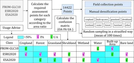
On taking the mean of 100 random samplings in a stratified manner as a reference, ESA2020 was found to have the highest OA (81.11%), followed by ESRI2020 (79.99%) and FROM_GLC10 (75.43%). In terms of single-class accuracy, the cropland, forest, and built-up areas in the three products all had higher accuracies, while the shrubland, wetland, and bare land areas all had lower PA and UA values.

(2)

Differences in classification standards are a major problem in the production of the current land cover products, and the unclear definition of a certain land cover class tends to lead to complete confusion during the classification. Land cover producers should pay particular attention to creating a single classification standard.

(3)

The sampling method affects the validation results. Both stratification and consideration of the class area ratio are important.

(4)

According to the different mixing ratios of the field collection points and the manual densification points, we found that the validation accuracy of the sample points close to the road and the uniform distribution of the sample points have a deviation of nearly 19%.

(5)

The accuracy of a class differed in different products, and each had its advantages and disadvantages. The overall accuracy of the cropland, forest, and built-up areas in the three land cover products; the accuracy of the grassland area in ESA2020; and the accuracy of the water area in ESRI2020 and ESA2020 exceeded 50%. From the perspective of the PA, we recommend that when producing land cover maps, the built-up area be extracted using FROM_GLC10. For cropland, forest, grassland, wetland, and bare land, ESRI2020 is more applicable. ESA2020 applies to shrubland and water. According to the UA, we recommend that users use these three land cover products comprehensively, for example, the cropland and water areas of FROM_GLC10; the shrubland and built-up areas of ESRI2020; and the forest, grassland, wetland, and bare land areas of ESA2020.

References

1. Din, S.U.; Mak, H.W.L. Retrieval of Land-Use/Land Cover Change (LUCC) Maps and Urban Expansion Dynamics of Hyderabad, Pakistan via Landsat Datasets and Support Vector Machine Framework. Remote Sens. 2021, 13, 3337. [Google Scholar] [CrossRef]
2. Yu, W.; Zang, S.; Wu, C.; Liu, W.; Na, X. Analyzing and modeling land use land cover change (LUCC) in the Daqing City, China. Appl. Geogr. 2011, 31, 600–608. [Google Scholar] [CrossRef]
3. Borrelli, P.; Robinson, D.A.; Fleischer, L.R.; Lugato, E.; Ballabio, C.; Alewell, C.; Meusburger, K.; Modugno, S.; Schütt, B.; Ferro, V. An validation of the global impact of 21st century land use change on soil erosion. Nat. Commun. 2017, 8, 2013. [Google Scholar] [CrossRef] [PubMed] [Green Version]
4. He, C.; Zhang, J.; Liu, Z.; Huang, Q. Characteristics and progress of land use/cover change research during 1990–2018. J. Geogr. Sci. 2022, 32, 537–559. [Google Scholar] [CrossRef]
5. Gong, P.; Wang, J.; Yu, L.; Zhao, Y.; Zhao, Y.; Liang, L.; Niu, Z.; Huang, X.; Fu, H.; Liu, S. Finer resolution observation and monitoring of global land cover: First mapping results with Landsat TM and ETM+ data. Int. J. Remote Sens. 2013, 34, 2607–2654. [Google Scholar] [CrossRef] [Green Version]
6. Zhou, G.; Wei, X.; Chen, X.; Zhou, P.; Liu, X.; Xiao, Y.; Sun, G.; Scott, D.F.; Zhou, S.; Han, L. Global pattern for the effect of climate and land cover on water yield. Nat. Commun. 2015, 6, 5918. [Google Scholar] [CrossRef] [Green Version]
7. Yuan, Q.; Shen, H.; Li, T.; Li, Z.; Li, S.; Jiang, Y.; Xu, H.; Tan, W.; Yang, Q.; Wang, J.; et al. Deep learning in environmental remote sensing: Achievements and challenges. Remote Sens. Environ. 2020, 241, 111716. [Google Scholar] [CrossRef]
8. Zhu, X.X.; Tuia, D.; Mou, L.; Xia, G.-S.; Zhang, L.; Xu, F.; Fraundorfer, F.; Magazine, R.S. Deep learning in remote sensing: A comprehensive review and list of resources. IEEE Geosci. Remote Sens. Mag. 2017, 5, 8–36. [Google Scholar] [CrossRef] [Green Version]
9. Maxwell, A.E.; Warner, T.A.; Fang, F. Implementation of machine-learning classification in remote sensing: An applied review. Int. J. Remote Sens. 2018, 39, 2784–2817. [Google Scholar] [CrossRef] [Green Version]
10. Gong, P.; Liu, H.; Zhang, M.; Li, C.; Wang, J.; Huang, H.; Clinton, N.; Ji, L.; Li, W.; Bai, Y.; et al. Stable classification with limited sample: Transferring a 30-m resolution sample set collected in 2015 to mapping 10-m resolution global land cover in 2017. Sci. Bull. 2019, 64, 370–373. [Google Scholar] [CrossRef]
11. Karra, K.; Kontgis, C.; Statman-Weil, Z.; Mazzariello, J.C.; Mathis, M.; Brumby, S.P. Global land use/land cover with Sentinel 2 and deep learning. In Proceedings of the 2021 IEEE International Geoscience and Remote Sensing Symposium IGARSS, Brussels, Belgium, 11–16 July 2021; pp. 4704–4707. [Google Scholar]
12. Kibria, M.G.; Nguyen, K.; Villardi, G.P.; Zhao, O.; Ishizu, K.; Kojima, F. Big data analytics, machine learning, and artificial intelligence in next-generation wireless networks. Kibria M G, Nguyen K, Villardi G P, et al. Big data analytics, machine learning, and artificial intelligence in next-generation wireless networks. IEEE Access 2018, 6, 32328–32338. [Google Scholar] [CrossRef]
13. Wu, J.; Guo, S.; Li, J.; Zeng, D. Big data meet green challenges: Big data toward green applications. IEEE Syst. J. 2016, 10, 888–900. [Google Scholar] [CrossRef]
14. Stoian, A.; Poulain, V.; Inglada, J.; Poughon, V.; Derksen, D. Land cover maps production with high resolution satellite image time series and convolutional neural networks: Adaptations and limits for operational systems. Remote Sens. 2019, 11, 1986. [Google Scholar] [CrossRef] [Green Version]
15. Tsendbazar, N.; Herold, M.; De Bruin, S.; Lesiv, M.; Fritz, S.; Van De Kerchove, R.; Buchhorn, M.; Duerauer, M.; Szantoi, Z.; Pekel, J.-F. Developing and applying a multi-purpose land cover validation dataset for Africa. Remote Sens. Environ. 2018, 219, 298–309. [Google Scholar] [CrossRef] [Green Version]
16. Venter, Z.S.; Barton, D.N.; Chakraborty, T.; Simensen, T.; Singh, G. Global 10 m Land Use Land Cover Datasets: A Comparison of Dynamic World, World Cover and Esri Land Cover. Remote Sens. 2022, 14, 4101. [Google Scholar] [CrossRef]
17. Giri, C.; Zhu, Z.; Reed, B. A comparative analysis of the Global Land Cover 2000 and MODIS land cover data sets. Remote Sens. Environ. 2005, 94, 123–132. [Google Scholar] [CrossRef]
18. Zhao, J.; Dong, Y.; Zhang, M.; Huang, L. Comparison of identifying land cover tempo-spatial changes using GlobCover and MCD12Q1 global land cover products. Arab. J. Geosci. 2020, 13, 1–12. [Google Scholar] [CrossRef]
19. Kang, J.; Yang, X.; Wang, Z.; Cheng, H.; Wang, J.; Tang, H.; Li, Y.; Bian, Z.; Bai, Z. Comparison of Three Ten Meter Land Cover Products in a Drought Region: A Case Study in Northwestern China. Land 2022, 11, 427. [Google Scholar] [CrossRef]
20. Wang, J.; Yang, X.; Wang, Z.; Cheng, H.; Kang, J.; Tang, H.; Li, Y.; Bian, Z.; Bai, Z. Consistency Analysis and Accuracy Validation of Three Global Ten-Meter Land Cover Products in Rocky Desertification Region—A Case Study of Southwest China. ISPRS Int. J. Geo-Inf. 2022, 11, 202. [Google Scholar] [CrossRef]
21. Chang, C.-P.; Wang, Z.; McBride, J.; Liu, C.-H. Annual cycle of Southeast Asia—Maritime Continent rainfall and the asymmetric monsoon transition. J. Clim. 2005, 18, 287–301. [Google Scholar] [CrossRef]
22. Hall, R.J.B.-B. Southeast Asia’s changing palaeogeography. Blumea-Biodivers. Evol. Biogeogr. Plants 2009, 54, 148–161. [Google Scholar] [CrossRef] [Green Version]
23. Paradis, E. Forest gains and losses in Southeast Asia over 27 years: The slow convergence towards reforestation. For. Policy Econ. 2021, 122, 102332. [Google Scholar] [CrossRef]
24. Rahman, M.S.; Khan, M.; Jolly, Y.; Kabir, J.; Akter, S.; Salam, A. Assessing risk to human health for heavy metal contamination through street dust in the Southeast Asian Megacity: Dhaka, Bangladesh. Sci. Total Environ. 2019, 660, 1610–1622. [Google Scholar] [CrossRef] [PubMed]
25. Plummer, M.G.; Morgan, P.J.; Wignaraja, G. Connecting Asia: Infrastructure for Integrating South and Southeast Asia; Edward Elgar Publishing: Cheltenham, UK, 2016. [Google Scholar]
26. Yu, H. China’s Belt and Road Initiative and its implications for Southeast Asia. Asia Policy 2017, 24, 117–122. [Google Scholar] [CrossRef]
27. Lam, J.S.L.; Cullinane, K.P.B.; Lee, P.T.-W. The 21st-century Maritime Silk Road: Challenges and opportunities for transport management and practice. Transp. Rev. 2018, 38, 413–415. [Google Scholar] [CrossRef] [Green Version]
28. Weber, N. Malays in the Indochinese Peninsula: Adventurers, Warlords and Ministers. J. Malays. Branch R. Asiat. Soc. 2021, 94, 1–23. [Google Scholar] [CrossRef]
29. Xu, L.; Sun, S.; Chen, H.; Chai, R.; Wang, J.; Zhou, Y.; Ma, Q.; Chotamonsak, C.; Wangpakapattanawong, P. Changes in the reference evapotranspiration and contributions of climate factors over the Indo–China Peninsula during 1961–2017. Int. J. Clim. 2021, 41, 6511–6529. [Google Scholar] [CrossRef]
30. Ohtani, M.; Tani, N.; Ueno, S.; Uchiyama, K.; Kondo, T.; Lee, S.L.; Ng, K.K.S.; Muhammad, N.; Finkeldey, R.; Gailing, O.; et al. Genetic structure of an important widely distributed tropical forest tree, Shorea parvifolia, in Southeast Asia. Tree Genet. Genomes 2021, 17, 1–13. [Google Scholar] [CrossRef]
31. Lord, F. Transformation to sustainable and resilient urban futures in Southeast Asia. ISPRS Ann. Photogramm. Remote Sens. Spat. Inf. Sci. 2020, 6, 43–50. [Google Scholar] [CrossRef]
32. Wang, C.; Wang, D.; Abbas, J.; Duan, K.; Mubeen, R. Global financial crisis, smart lockdown strategies, and the COVID-19 spillover impacts: A global perspective implications from Southeast Asia. Front. Psychiatry 2021, 12, 643783. [Google Scholar] [CrossRef]
33. Sovacool, B. The political economy of oil and gas in Southeast Asia: Heading towards the natural resource curse? Pac. Rev. 2010, 23, 225–259. [Google Scholar] [CrossRef]
34. Kumar, S. Validation of renewables for energy security and carbon mitigation in Southeast Asia: The case of Indonesia and Thailand. Appl. Energy 2016, 163, 63–70. [Google Scholar] [CrossRef]
35. Clay, J. World Agriculture and the Environment: A Commodity-by-Commodity Guide to Impacts and Practices; Island Press: Washington, DC, USA, 2004. [Google Scholar]
36. Hasan, M.H.; Mahlia, T.I.; Nur, H.J.R.; Reviews, S.E. A review on energy scenario and sustainable energy in Indonesia. Renew. Sustain. Energy Rev. 2012, 16, 2316–2328. [Google Scholar] [CrossRef]
37. Liu, Q.; Wu, J.; Li, L.; Yu, L.; Li, J.; Xin, X. Ecological environment monitoring for sustainable development goals in the Belt and Road region. AOGEOSS Prog. 2018, 22, 686–708. [Google Scholar]
38. Huang, B.; Hu, X.; Fuglstad, G.-A.; Zhou, X.; Zhao, W.; Cherubini, F. Predominant regional biophysical cooling from recent land cover changes in Europe. Nat. Commun. 2020, 11, 1066. [Google Scholar] [CrossRef] [PubMed] [Green Version]
39. Yu, L.; Wang, J.; Li, X.; Li, C.; Zhao, Y.; Gong, P. A multi-resolution global land cover dataset through multisource data aggregation. Sci. China Earth Sci. 2014, 57, 2317–2329. [Google Scholar] [CrossRef]
40. Zhao, Y.; Gong, P.; Yu, L.; Hu, L.; Li, X.; Li, C.; Zhang, H.; Zheng, Y.; Wang, J.; Zhao, Y. Towards a common validation sample set for global land-cover mapping. Int. J. Remote Sens. 2014, 35, 4795–4814. [Google Scholar] [CrossRef]
41. Li, C.; Gong, P.; Wang, J.; Zhu, Z.; Biging, G.S.; Yuan, C.; Hu, T.; Zhang, H.; Wang, Q.; Li, X. The first all-season sample set for mapping global land cover with Landsat-8 data. Sci. Bull. 2017, 62, 508–515. [Google Scholar] [CrossRef] [Green Version]
42. Olofsson, P.; Foody, G.M.; Stehman, S.V.; Woodcock, C.E. Making better use of accuracy data in land change studies: Estimating accuracy and area and quantifying uncertainty using stratified estimation. Remote Sens. Environ. 2013, 129, 122–131. [Google Scholar] [CrossRef]
43. Zanaga, D.; Van De Kerchove, R.; De Keersmaecker, W.; Souverijns, N.; Brockmann, C.; Quast, R.; Wevers, J.; Grosu, A.; Paccini, A.; Vergnaud, S.; et al. ESA WorldCover 10 m 2020 v100. Zenodo 2021, 601280. [Google Scholar] [CrossRef]
44. Powell, R.; Matzke, N.; de Souza Jr, C.; Clark, M.; Numata, I.; Hess, L.; Roberts, D. Sources of error in accuracy validation of thematic land-cover maps in the Brazilian Amazon. Remote Sens. Environ. 2004, 90, 221–234. [Google Scholar] [CrossRef]
45. Ruelland, D.; Tribotte, A.; Puech, C.; Dieulin, C. Comparison of methods for LUCC monitoring over 50 years from aerial photographs and satellite images in a Sahelian catchment. Int. J. Remote Sens. 2011, 32, 1747–1777. [Google Scholar] [CrossRef]
46. Lee, S. Application of logistic regression model and its validation for landslide susceptibility mapping using GIS and remote sensing data. Int. J. Remote Sens. 2005, 26, 1477–1491. [Google Scholar] [CrossRef]
47. Lu, M.; Wu, W.; Zhang, L.; Liao, A.; Peng, S.; Tang, H. A comparative analysis of five global cropland datasets in China. Sci. China Earth Sci. 2016, 59, 2307–2317. [Google Scholar] [CrossRef]
48. Xu, Y.; Yu, L.; Feng, D.; Peng, D.; Li, C.; Huang, X.; Lu, H.; Gong, P. Comparisons of three recent moderate resolution African land cover datasets: CGLS-LC100, ESA-S2-LC20, and FROM-GLC-Africa30. Int. J. Remote Sens. 2019, 40, 6185–6202. [Google Scholar] [CrossRef]
49. Hua, T.; Zhao, W.; Liu, Y.; Wang, S.; Yang, S. Spatial consistency validations for global land-cover datasets: A comparison among GLC2000, CCI LC, MCD12, GLOBCOVER and GLCNMO. Remote Sens. 2018, 10, 1846. [Google Scholar] [CrossRef] [Green Version]
50. Wu, W.; Shibasaki, R.; Yang, P.; Ongaro, L.; Zhou, Q.; Tang, H. Validation and comparison of 1 km global land cover products in China. Int. J. Remote Sens. 2008, 29, 3769–3785. [Google Scholar] [CrossRef]
51. Congalton, R.G.; Green, K. Assessing the Accuracy of Remotely Sensed Data: Principles and Practices; CRC Press: Boca Raton, FL, USA, 2019. [Google Scholar]
52. Congalton, R. A review of assessing the accuracy of classifications of remotely sensed data. Remote Sens. Environ. 1991, 37, 35–46. [Google Scholar] [CrossRef]
53. Olofsson, P.; Foody, G.M.; Herold, M.; Stehman, S.V.; Woodcock, C.E.; Wulder, M.A. Good practices for estimating area and assessing accuracy of land change. Remote Sens. Environ. 2014, 148, 42–57. [Google Scholar] [CrossRef]
54. Horvitz, D.G.; Thompson, D.J. A generalization of sampling without replacement from a finite universe. J. Am. Stat. Assoc. 1952, 47, 663–685. [Google Scholar] [CrossRef]
55. Neyman, J. On the two different aspects of the representative method: The method of stratified sampling and the method of purposive selection. In Breakthroughs in Statistics; Springer: Berlin/Heidelberg, Germany, 1992; pp. 123–150. [Google Scholar]
56. Stehman, S.V. Estimating area and map accuracy for stratified random sampling when the strata are different from the map classes. Int. J. Remote Sens. 2014, 35, 4923–4939. [Google Scholar] [CrossRef]
57. Stehman, S.V. Sampling designs for accuracy validation of land cover. Int. J. Remote Sens. 2009, 30, 5243–5272. [Google Scholar] [CrossRef]
58. Tsendbazar, N.; Herold, M.; Li, L.; Tarko, A.; de Bruin, S.; Masiliunas, D.; Lesiv, M.; Fritz, S.; Buchhorn, M.; Smets, B.; et al. Towards operational validation of annual global land cover maps. Remote Sens. Environ. 2021, 266, 112686. [Google Scholar] [CrossRef]
59. Negassa, M.D.; Mallie, D.T.; Gemeda, D.O. Forest cover change detection using Geographic Information Systems and remote sensing techniques: A spatio-temporal study on Komto Protected forest priority area, East Wollega Zone, Ethiopia. Environ. Syst. Res. 2020, 9, 1. [Google Scholar] [CrossRef] [Green Version]
60. Townsend, J.T. Theoretical analysis of an alphabetic confusion matrix. Percept. Psychophys. 1971, 9, 40–50. [Google Scholar] [CrossRef]
61. Visa, S.; Ramsay, B.; Ralescu, A.L.; Van Der Knaap, E. Confusion matrix-based feature selection. MAICS 2011, 710, 120–127. [Google Scholar]
62. Hay, A. The derivation of global estimates from a confusion matrix. Int. J. Remote Sens. 1988, 9, 1395–1398. [Google Scholar] [CrossRef]
63. Luque, A.; Carrasco, A.; Martín, A.; de las Heras, A. The impact of class imbalance in classification performance metrics based on the binary confusion matrix. Pattern Recognit. 2019, 91, 216–231. [Google Scholar] [CrossRef]
64. Maxwell, A.E.; Warner, T.A.; Guillén, L.A. Accuracy validation in convolutional neural network-based deep learning remote sensing studies—Part 2: Recommendations and best practices. Remote Sens. 2021, 13, 2591. [Google Scholar] [CrossRef]
65. Maxwell, A.E.; Warner, T.A.; Guillén, L.A. Accuracy validation in convolutional neural network-based deep learning remote sensing studies—Part 1: Literature review. Remote Sens. 2021, 13, 2450. [Google Scholar] [CrossRef]
66. Pontius, R.G., Jr.; Millones, M. Death to Kappa: Birth of quantity disagreement and allocation disagreement for accuracy validation. Int. J. Remote Sens. 2011, 32, 4407–4429. [Google Scholar] [CrossRef]
67. Benjamini, Y. Opening the box of a boxplot. Am. Stat. 1988, 42, 257–262. [Google Scholar]
68. Frigge, M.; Hoaglin, D.C.; Iglewicz, B. Some implementations of the boxplot. Am. Stat. 1989, 43, 50–54. [Google Scholar]
69. Rousseeuw, P.J.; Ruts, I.; Tukey, J.W. The bagplot: A bivariate boxplot. Am. Stat. 1999, 53, 382–387. [Google Scholar]
70. Congalton, R.G. A comparison of sampling schemes used in generating error matrices for assessing the accuracy of maps generated from remotely sensed data. Photogramm. Eng. Remote Sens. 1988, 54, 593–600. [Google Scholar]
71. Stehman, S.V.; Olofsson, P.; Woodcock, C.E.; Herold, M.; Friedl, M.A. A global land-cover validation data set, II: Augmenting a stratified sampling design to estimate accuracy by region and land-cover class. Int. J. Remote Sens. 2012, 33, 6975–6993. [Google Scholar] [CrossRef]
72. Di Gregorio, A. Land Cover Classification System: Classification Concepts and User Manual: LCCS; Food & Agriculture Org.: Yokohama, Japan, 2005; Volume 2. [Google Scholar]
73. Xie, Y.; Sha, Z.; Yu, M. Remote sensing imagery in vegetation mapping: A review. J. Plant Ecol. 2008, 1, 9–23. [Google Scholar] [CrossRef]
74. He, C.; Zhang, Q.; Li, Y.; Li, X.; Shi, P. Zoning grassland protection area using remote sensing and cellular automata modeling—a case study in Xilingol steppe grassland in northern China. J. Arid. Environ. 2005, 63, 814–826. [Google Scholar] [CrossRef]
75. Stow, D.; Hamada, Y.; Coulter, L.; Anguelova, Z. Monitoring shrubland habitat changes through object-based change identification with airborne multispectral imagery. Remote Sens. Environ. 2008, 112, 1051–1061. [Google Scholar] [CrossRef]
76. Rendenieks, Z.; Tērauds, A.; Nikodemus, O.; Brūmelis, G. Comparison of input data with different spatial resolution in landscape pattern analysis–a case study from northern latvia. Appl. Geogr. 2017, 83, 100–106. [Google Scholar] [CrossRef]
77. Olofsson, P.; Stehman, S.V.; Woodcock, C.E.; Sulla-Menashe, D.; Sibley, A.M.; Newell, J.D.; Friedl, M.A.; Herold, M. A global land-cover validation data set, part I: Fundamental design principles. Int. J. Remote Sens. 2012, 33, 5768–5788. [Google Scholar] [CrossRef]
78. Kang, J.; Wang, Z.; Sui, L.; Yang, X.; Ma, Y.; Wang, J. Consistency analysis of remote sensing land cover products in the tropical rainforest climate region: A case study of Indonesia. Remote Sens. 2020, 12, 1410. [Google Scholar] [CrossRef]
Figure 1. Location and topography of Southeast Asia.
Remotesensing 14 05053 g001
Figure 2. Field collecting routes in Southeast Asia.
Remotesensing 14 05053 g002
Figure 3. Processing flow and spatial distribution of 3326 field collection points: 1171 cropland points, 1133 forest points, 388 grassland points, 138 shrubland points, 64 wetland points, 94 water points, 208 built-up area points, and 130 bare land points.
Remotesensing 14 05053 g003
Figure 4. Method flow of validation point processing based on consistency analysis.
Remotesensing 14 05053 g004
Figure 5. Comparison results with the different sampling experiments.
Remotesensing 14 05053 g005
Figure 6. Comparison of the areas of each land cover class in the three land cover products.
Remotesensing 14 05053 g006
Figure 7. Distribution of the field collection points and consistent manual densification points. There are 18,134 points in total, including 3326 field collection points and 14,808 manual densification points. Among the manual densification points, there are 3971 cropland points, 6883 forest points, 1238 grassland points, 1061 shrubland points, 189 wetland points, 645 water points, 552 built-up area points, and 263 bare land points.
Remotesensing 14 05053 g007
Figure 8. Overall accuracy values calculated with 100 samples.
Remotesensing 14 05053 g008
Figure 9. Accuracy of the eight main classes: cropland (CL), forest (FR), grassland (GL), shrubland (SL), wetland (WL), water (WT), built-up area (BA), and bare land (BL). (a) Mean PA values of the three land cover products, and (b) mean UA values of the three land cover products.
Remotesensing 14 05053 g009
Figure 10. Boxplots of the OA, PA, and UA values. (a) Boxplot of the OA values of 100 samples for the three products. (b,c) Boxplots of the individual classes for the three products sampled 100 times, including built-up area (BA), bare land (BL), cropland (CL), forest (FR), grassland (GL), shrubland (SL), wetland (WL), and water (WT).
Remotesensing 14 05053 g010
Figure 11. The mean OA value of 100 samples for the different mixing ratios of the field collection points and the manual densification points.
Remotesensing 14 05053 g011
Figure 12. Suggestions for each class. Blue indicates that it meets our validation criteria, that is, the UA and the PA of a single class both reach 50%. The check marks indicate the highest PA (pink) and UA (green) values for each class among the three land cover products.
Remotesensing 14 05053 g012