Article

An Oblique Projection-Based Beamforming Method for Coherent Signals Receiving

1
National Laboratory of Radar Signal Processing, Xidian University, Xi’an 710071, China
2
Hangzhou Institute of Technology, Xidian University, Hangzhou 311200, China
3
School of Microelectronics and Communication Engineering, Chongqing University, Chongqing 400044, China
*
Author to whom correspondence should be addressed.
Remote Sens. 2022, 14(19), 5043; https://doi.org/10.3390/rs14195043
Submission received: 25 August 2022 / Revised: 25 September 2022 / Accepted: 4 October 2022 / Published: 9 October 2022

Abstract

:
Within a complex sea or ground surface background, multipath signals are strongly correlated or even completely coherent, which leads to signal cancellation when conventional optimal beamforming is performed. Aiming at the above problem, a coherent signal-receiving algorithm is proposed based on oblique projection technology in this paper. The direction of arrival (DOA) of incident signals is estimated firstly by the space smoothing-based MUSIC method. The composite steering vector of multipath coherent signals is then obtained utilizing the oblique projection matrix constructed with the estimated angles. The weight vector is thereby derived with the minimum variance distortionless response criteria. The proposed oblique projection-based beamformer can receive the multipath coherent signals effectively. Moreover, the proposed beamformer is more robust and converges to optimal beamformer rapidly without aperture loss. The theoretical analysis and simulation verify the validity and superiority of the proposed coherent signal beamformer.

1. Introduction

In the 1840s, the concept of radio detection and ranging (radar) was put forward by Christian Andreas Doppler. Since then, the study of radar has been uninterrupted, and has been developed rapidly. As an important means of remote sensing, radar, benefitting from its characteristics of working for full-weather and full-time, has not only played an indispensable role in the military field, but also extensively applied in various civil applications (weather forecast [1], resource exploration [2], environmental monitoring [3], etc.) and scientific researches [4] (astronomical object, atmospheric physics, ionospheric structure, etc.). In the process of radar development, various kinds of radar have been derived, such as early warning radar, weather radar, spaceborne and airborne synthetic aperture radar (SAR), etc. In the late 1930s, the presentation of phased array radar promoted a great development of radar technology. The phase array radar technology has been widely used in many practical applications with a high degree of excellence such as flexible controllable beam and multi-targets surveillance.
As an important research branch in the field of signal processing, array signal processing technology has the rapidly developed in two aspects of theoretical research and practical application since the 1960s, which cover the application scope of radar, communications, sonar telemetry, radio astronomy, biological medical [5,6,7], and many other fields. Beamforming, an important research content of array signal processing, can achieve directional selectivity by processing the data collected by array sensors in the spatial domain. Therefore, beamforming is also called spatial filtering. The purpose of beamforming is to align the main lobe of the antenna beam pattern with the desired signal by changing the weight vector on the array antenna, meanwhile suppressing interferences to improve the output signal to interference plus noise ratio (SINR). Adaptive beamforming technology can adaptively change the weight vector according to the signal environment, which can obtain better output performance.
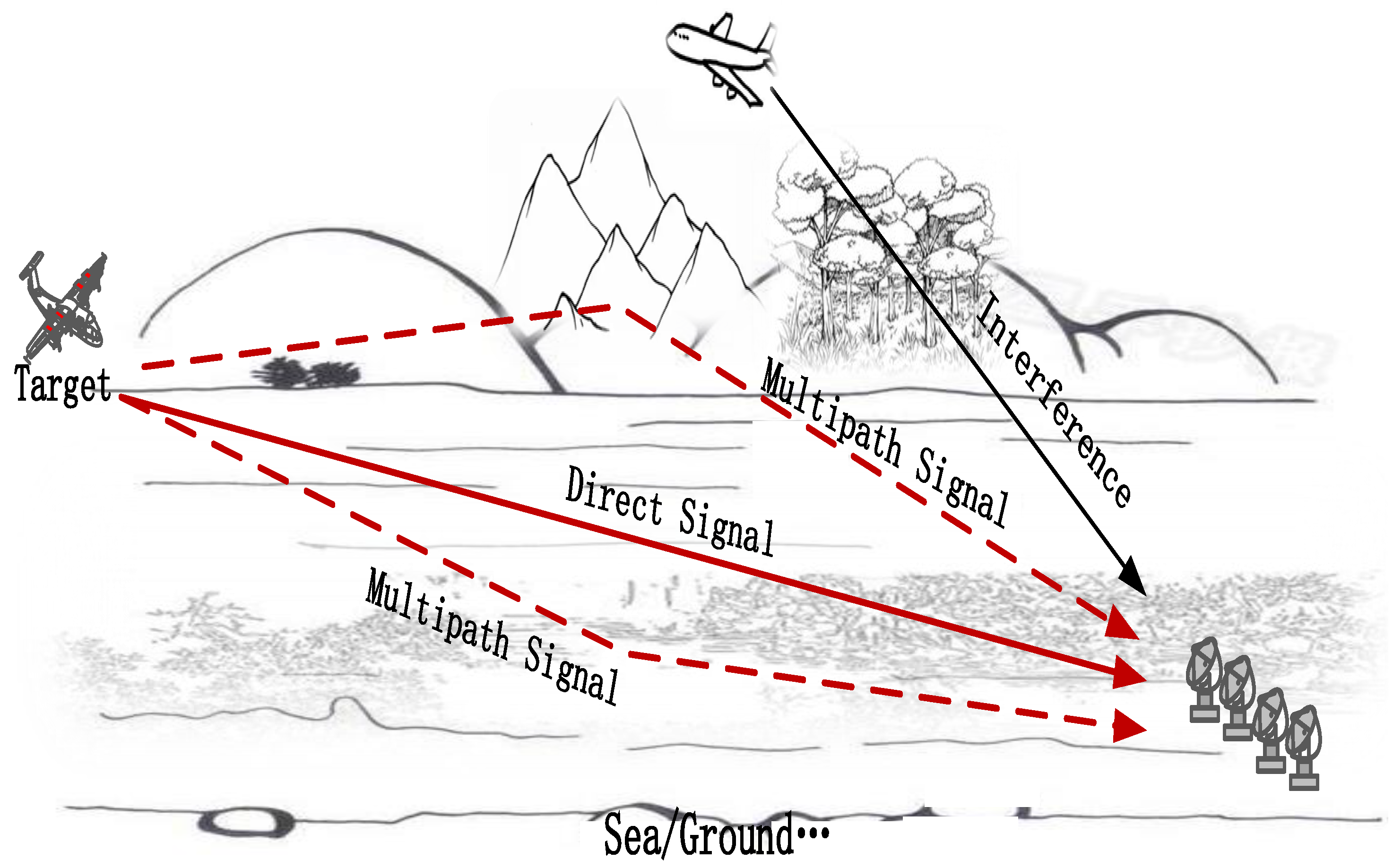
However, the desired target echo signals are strongly correlated or even completely coherent with multipath signals in complex scenes, such as the low-altitude targets surveillance within sea/ground surface or urban background, which brings severe challenges to radar target signal receiving, detecting and tracking. The multipath effect [8,9] refers to the electromagnetic wave transmission through different paths. Besides the direct path from the source to the receiving end, the electromagnetic wave propagation path also includes more than the rest of the transmission path. When the received signals are uncorrelated, the traditional adaptive beamforming methods [10,11,12], such as minimum variance distortionless response (MVDR) [13] and Minimum Mean Square Error (MMSE), can effectively receive the target signal while suppressing the irrelevant interference signal, so as to output the maximum SINR. However, in a multipath environment, the target signal has multiple receiving paths, and the received signals of different paths are highly correlated, or even coherent. The direct signal and reflected signal are superimposed according to their respective phases at the receiver, resulting in distortion or error of the target signal. As a result, the performance of traditional beamforming technology deteriorates dramatically in a multipath environment [14]. Signal attenuation and delay caused by the multipath effect directly affect the target detection, tracking and recognition performance of electronic reconnaissance equipment, so it has been widely studied by experts and scholars in the radar field. In the 1950s, a large amount of theoretical and experimental research was carried out on the problems caused by the multipath effect, mainly analyzing the characteristics of a low altitude target echo and multipath reflection [15,16]. In the 1970s, experts began to build low-altitude echo models to suppress and separate multipath signals.
For the beamforming problem in the multipath coherence case, the early research mainly focused on the direct signal reception, regarding other multipath signals as interferences. Reducing the correlationship of the correlated signals and performing conventional adaptive beamforming is a typical kind of method to suppress the coherent interference. In reference [17], the classical spatial smoothing was proposed to recover the rank of the signal plus interference subspace, which divided the full array into overlapping subarrays with equal number elements and ultimately obtained the averaged subarray correlation matrix. To improve the decorrelation performance, all the elements of the averaged subarray correlation matrix were averaged along its diagonals to restore its Toeplitz structure in [18]. In reference [19], an adaptive spatial smoothing algorithm was present to improve the array output gain when the angle between the interference source and the desired signal was small. The robust beamforming methods were proposed based on the spatial smooth considering the steering vector errors and correlation matrix errors in reference [20]. Other spatial smoothing methods are present for coherent interference suppression in reference [21,22,23,24,25].
Although the spatial smoothing methods reduced the signal correlation, they suffered from the array gain loss with the decrease of effective aperture. The method proposed in [26] constructed a weight vector to minimize the output power and put null in the coherent multipath direction so as to suppress the coherent interference and avoid signal cancellation. However, the method needed to estimate the incident angle of the coherent signals in advance. In [27], a transformation was constructed based on the DOA estimation results to remove the signal in the desired direction and preserve the coherent interference. Then beamforming was performed on the transformed signal which contained only coherent multipath interference, irrelevant interference and noise, and thus the signal cancellation was also avoided. The reference [28] eliminated the signal of the desired direction by using the Duvall structure. In this way, the computation cost was reduced. The method in [29,30,31] reconstructed the covariance matrix to satisfy the Toeplitz property. Compared with spatial smoothing methods, these methods have the advantage of retaining full aperture, but there are many influencing factors and large estimation errors.
Although the above methods can solve the signal cancellation problem in the case of coherentsignal beamforming, they only take the direct signal as the useful signal in the beamforming process, which can not make full use of the multipath signal. The signal energy is lost and the maximum output SINR cannot be reached. Therefore, the other strategy of coherent signal beamforming is to take the multipath signal as the useful signal like the direct signal. In reference [32], an adaptive weight vector was obtained for coherent signal receiving based on the composite steering vector of coherent multipath signals estimated by utilizing the transformation matrix which was constructed by the DOA of uncorrelated interference. Two beamforming algorithms were present in [33] with forcing the array responses to the pre-estimated angle clusters of the coherent multipath signal no less than unity while minimising the output power. A coherent beamforming method was proposed in [34] with the multiple coherent signals’ DOA information known, which optimized the covariance matrix and constrained the beam mainlobe magnitude of multiple coherent signals to obtain the optimal weight vector. It is essential that the coherent signals and irrelevant interference should be distinguished from the DOA estimation results. Based on the anti-diagonal unit matrix, the reference [35] constructed a new covariance matrix and obtained the weight vector according to the MVDR criterion, which broke the reverse relationship of the output phases between direct and multipath signal to avoid signal cancellation. However, the method is not robust. Using the subaperture weight vector of the spatial smoothing beamformer (SSB) mentioned in [17], the eigenspace-based beamformer (ESB) proposed in [36] extracted the composite steering vector of the coherent signal, and further obtained the MVDR optimal weight vector to combine the multipath signals. In the article [37], the desired signal was obtained with noise and firstly utilized a subtraction-based MVDR beamformer, which was fed back to the original full aperture array to perform the MMSE beamformer.
In order to solve the problem of signal cancellation with traditional beamforming with multipath coherent signals, an oblique projection-based beamforming method for coherent signal receiving is proposed in this paper, which can effectively suppress irrelevant interference and improve the output SINR by combining coherent signals. Firstly, spatial smoothing is performed to reduce the coherence of multipath signals. Secondly, DOA estimation is obtained by conducting the multiple signal classification (MUSIC) algorithm covariance matrix. Then, the oblique projection matrix is constructed to extract the composite steering vector of the multipath coherent signals. Finally, the weight vector of the proposed oblique projection-based beamformer is derived with the minimum variance distortionless response criteria. The proposed beamforming is implemented with the full aperture of the array. What’s more, it can effectively combine multipath coherent signals, and converges to optimal beamformer rapidly.
This paper is organized as follows. Section 2 builds the general array signal model in coherent multipath case with interference. The optimal beamforming method MVDR and DOA estimation based on spatial smoothing are dealt with in Section 3. The proposed oblique projection-based beamformer (OPB) algorithm is introduced in Section 4. The theoretical performance and the numerical simulation results are provided in Section 5 and Section 6, respectively. Section 7 draws the conclusion.

2. Signal Model

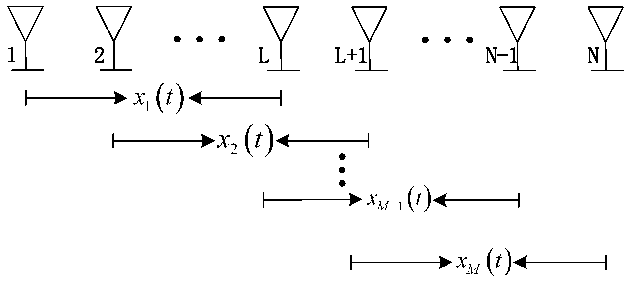
A linear array, with N elements equally spaced with spacing d, is considered in this paper. Due to the multipath effect, the received target signal consists of K + 1 coherent signals with DOAs { θ i } i = 0 K . In addition, the received signal contains P uncorrelated interferences with DOAs { θ j } j = 1 P . As is shown in Figure 1, the received signal data of the nth element for time t is represented by x N ( t ) . Then the received signal vector of the whole array, denoted by x ( t ) , can be expressed as
x ( t ) = x 1 ( t ) x 2 ( t ) x N ( t ) T = i = 0 K ρ i a N ( θ i ) s d ( t ) + j = 1 P a N ( θ j ) s j ( t ) + n N ( t )
where P + K + 1 < N . ρ i , i = 0 , , K , is the reflection coefficient of i t h path of the target signals. And generally, the reflection coefficient form direction θ 0 is assumed ρ 0 = 1 . s d ( t ) , s j ( t ) ( j = 1 , , P ) , and n N ( t ) are the desired signal, the j t h uncorrelated interference signal and the additive white Gaussian noise with power σ n 2 , respectively. s d ( t ) , s j ( t ) and n N ( t ) are assumed uncorrelated mutually. a N ( θ ) stands for the N-dimension steering vector at the direction θ
a N ( θ ) = [ 1 e j 2 π d / λ   sin θ e j 2 π ( N 1 ) d / λ   sin θ ] T
The covariance matrix R x of received data x ( t ) can be expressed
R x = E x ( t ) x H ( t )
It should be noted that both the target and interference signal in the model are assumed far-field narrowband signals. Due to the influence of spatial dispersion and aperture traverse, the adaptive beamforming technique of the wideband signal is different from that of the narrowband signal. Here we emphasize the study of the narrowband adaptive beamforming algorithm.

3. Optimal Beamformer and Problem Statement

The basic principle of adaptive beamforming is that it can automatically adjust the amplitude and phase of the weight coefficient of the antenna array according to the receiving criterions so as to minimize the cost function and achieve the best receiving effect under the receiving criterions. MVDR and MMSE are two main criterions of adaptive beamforming to maximize the output SINR. Moreover, the two algorithms are equivalent when the noise is independent of the desired signal and the interference signal.

3.1. Optimal Beamformer

In the case of coherent multipath signals, given the direction of the direct signal, the optimal weight under the MVDR criterion can be obtained as [38]
w M V D R = η R x 1 a N ( θ 0 )
where θ 0 denote the direction of the direct signal. Due to the existence of coherent multipath signals, the optimal adaptive weight (4) will make all paths of the desired signals cancellation, resulting in almost no expected signals received [35]
w M V D R H k = 0 K ρ k a N ( θ k ) = 0
Therefore, in order to achieve the optimal beamforming, the composite steering vector must be obtained by the given of all the reflected signal angles and reflection coefficients of the expected signal, where the optimal weight is
w M V D R = η R x 1 a d
where a d = k = 0 K ρ k a N ( θ k ) denotes the composite steering vector of the expected signal. Substituting a d into (3) and rewriting the received data model as follows
x t = a d s d ( t ) + j = 1 P a N ( θ j ) s j ( t ) + n N ( t )
However, in the actual situation, the arrival angles and the reflection coefficients of all coherent signals cannot be obtained directly.

3.2. DOA Estimation Method Based on Spatial Smoothing

In recent years, there are many DOA estimation methods for coherent signals, such as the MUSIC method based on decorrelation, maximum likelihood, subspace fitting method, spatial sparse method, parameter estimation method based on Sparse Bayes, and so forth. Some of the above methods have strong space resolution ability. The MUSIC method has obvious advantages of high resolution, high precision and strong robustness, so it is adopted to realize the DOA estimation in this paper. Of course, the DOA estimation algorithm mentioned above can be selectively used in different environmental contexts. For example, when the DOA difference between coherent signals is small and the number of paths of coherent signals is large, DOA estimation algorithms without decoherence (such as parameter estimation method based on Sparse Bayes, etc.) can be adopted accordingly. Here is a brief introduction to forward spatial smoothing for coherent DOA estimation.
As shown in Figure 2, the array is divided into overlapping subarrays of size L according to the signal model shown in Equation (1). The total number of subarrays is M = N L + 1 . The signal model of the mth sub-array can be expressed as
X m ( t ) = x m ( t ) x m + 1 ( t ) x m + L 1 ( t ) T
And its corresponding covariance matrix is
R m = E x m ( t ) x m H ( t )
The MUSIC method based on the forward space smoothing restores the rank of the coherent signal covariance matrix by averaging the subarray covariance matrixes. Therefore, the covariance matrix modified by forward space smoothing is
R f = 1 M m = 1 M R m
If N P , the averaged covariance matrix R f is full rank when L P [39].
The eigenvector matrix U N of noise subspace can be obtained by eigen decomposition of R f . Therefore, DOA estimation can be realized by finding the minima of the following equation
θ M U S I C = arg min θ a L H ( θ ) U N U N H a L ( θ )
Generally, DOA estimation is performed equivalently by finding the maxima of the space spectrum
P M U S I C = 1 a L H ( θ ) U N U N H a L ( θ )

3.3. Orthogonal Projection and Oblique Projection

Supposing that Matrix C is a full column rank matrix of m × n dimension, the projection matrix P C of matrix C is obtained as follows according to projection theory,
P C = C [ C H C ] 1 C H
where matrix P C is the projection operator of the subspace S C represented by the column vectors of matrix C , and is the m-dimensional square matrix.
The orthogonal projection matrix of matrix C can be constructed as
P C = I m P C
where matrix P C is the projection operator of the orthogonal subspace S C , which is also an m-dimensional square matrix, I m is the m-dimensional identity matrix.
Similarly, given that matrix D is a m × k dimension with full column rank matrix, the rank of [ C , D ] is n + k . If n + k < m , the oblique projection matrix P D / C can be constructed
P D / C = D [ D H P C D ] 1 D H P C
where matrix P D / C is the projection operator onto the space S C along the space S D . According to the properties of oblique projection, there are
P D / C D = D
P D / C C = 0

4. The Proposed Approach: Oblique Projection-Based Beamformer (OPB)

The signal model in Equation (1) can be simplified to
x ( t ) = x 1 ( t ) x 2 ( t ) x N ( t ) T = i = 0 K ρ i a N ( θ i ) s d ( t ) + j = 1 P a N ( θ j ) s j ( t ) + n N ( t ) = A S ( t ) + n N ( t )
where A = [ a d a J ( θ 1 ) a J ( θ 2 ) a J ( θ P ) ] is the steering vector matrix, a d = i = 0 K ρ i a N ( θ i ) is the composite steering vector of the expected signal, S ( t ) = [ s d ( t ) s 1 ( t ) s P ( t ) ] T stands for the echo signal of the target and interference.
In addition, the interference steering vector matrix is expressed as
A J = a J ( θ 1 ) a J ( θ 2 ) a J ( θ P )
Then, A = a d A J , and the covariance matrix of the array can be written as
R x = E x ( t ) x H ( t ) = A R S A H + σ n 2 I N = [ a d A J ] σ d 2 0 1 × P 0 1 × P R J a d H A J H + σ n 2 I N
The steering vector matrix of all echo signals except the direct angle θ 0 can be written as
B = [ a ( θ 1 ) a ( θ 2 ) a ( θ K ) a J ( θ 1 ) a J ( θ 2 ) a J ( θ P ) ]
Based on the Equations (13) and (14), the projection matrix P B and orthogonal projection matrix P B of matrix B can be deduced.
P B = I N P B = I N B B H B 1 B H
In Equation (15), the projection matrix P a ( θ 0 ) / B is obtained along matrix B onto the space of vector a ( θ 0 ) .
P a ( θ 0 ) / B = a ( θ 0 ) a ( θ 0 ) H P B a ( θ 0 ) 1 a ( θ 0 ) H P B
The steering vectors at different angles are incoherent. According to the properties of oblique projection in Equations (16) and (17), if the matrix A is projected along B onto a ( θ 0 ) as follows, the output of oblique projection is given by
P a ( θ 0 ) / B A = P a ( θ 0 ) / B [ a d A J ] = P a ( θ 0 ) / B [ i = 0 K ρ i a N ( θ i ) A J ] = [ a ( θ 0 ) 0 0 ]
Then there are
a ( θ 0 ) H P a ( θ 0 ) / B A = [ N 0 0 ]
A R S A H P a ( θ 0 ) / B H a ( θ 0 ) = [ a d A J ] σ d 2 0 1 × P 0 1 × P R J N 0 1 × P = N σ d 2 a d
From the Equation (26), it is obvious that the composite steering vector a d is obtained, which is important for the following deduction of the optimal weight.
According to the adaptive weight vector (6) of optimal beamformer in Section 2, the above conclusion we have mentioned is that the optimal weight w M V D R can be obtained once given the composite steering vector. Therefore, the MVDR beamformer can be performed according to the above result.
w M V D R O P = R X 1 A R S A H P a ( θ 0 ) / B H a ( θ 0 )
According to the above weight vector W M V D R O P , the maximum signal to interference plus noise power ratio (SINR) can be obtained by beamforming. However, it is difficult to obtain A R S A H directly in practice. In the derivation process, it is apparent that the steering vector matrix A contains the composite steering vector a d , and it is very complicated to estimate the reflection coefficient. Moreover, R S is another puzzle. Therefore, it is unrealistic to estimate A R S A H .
From the Equation (20), A R S A H is the part of the received signal’s covariance matrix that removes the component of noise. So it can be extracted from the received signal’s covariance matrix R x . The eigenvalue decomposition of the covariance matrix R x is represented as
R X = E x ( t ) x H ( t ) } = A R S A H + σ n 2 I = U S Λ S U S H + U N Λ N U N H = i = 1 N λ i u i u i H
where λ 1 λ 2 λ P + 1 λ P + 2 = λ P + 3 = = λ N = σ n 2 are the eigenvalues of R X , and u i are their corresponding orthonormal eigenvectors. U S = [ u 1 , u 2 , , u P , u P + 1 ] is the signal plus interference subspace, which is composed of the corresponding eigenvectors of the first P + 1 great eigenvalues. Λ S is a ( P + 1 ) dimension diagonal matrix, whose diagonal elements are the eigenvalues of U S . Accordingly, U N = [ u P + 2 , u P + 3 , , u N ] is the noise subspace, which is composed of the corresponding eigenvectors of the rest eigenvalues. Λ N is a ( N P 1 ) dimension diagonal matrix, whose diagonal elements are σ n 2 .
Both U S and A represent the signal plus interference subspace of the received signal R X . Therefore, according to the subspace theory, the steering vector matrix A and the eigenvector matrix U S span the same subspace. Based on the theory, combined with Equation (13), the projection matrix of A can be obtained
P A = A [ A H A ] 1 A H = U S [ U S H U S ] 1 U S H = U S U S H
The projection of R X onto the subspace represented by the A is just the subspace of the signal plus the interference. It is, in fact,
A R S A H = P A R X = U S U S H R X
Substituting the Equation (30) into (27), the weight vector of the proposed oblique projection beamformer based on MVDR optimal criterion can be obtained
w O P = R X 1 [ U S U S H R X P a ( θ 0 ) / B H a ( θ 0 ) ] = U S U S H P a ( θ 0 ) / B H a ( θ 0 )
It is worth noting that all the above theoretical derivations are based on the assumption that the angles of the incident signals are known accurately. The DOA estimation method can be chosen as spatial smoothing-based MUSIC as introduced in Section 3.2 for the coherent case. Other DOA estimation methods can also be adopted, such as Sparse Bayes and other methods proposed in recent years, which are not limited by the coherent condition. By analyzing the Equations (24)–(26), it can be concluded that as long as the angle estimation of irrelevant interference is relatively accurate, the weight vector obtained by the Equation (31) still effectively receiving the combination of the multipath signals even when the angle estimation of the coherent signal are inaccurate or unsuccessful. It is worth emphasizing that there is no correlation between interference and target echo signal, so the angle estimation of interference is relatively simple. Suppose θ is the real angle, and θ ^ is the estimated angle. The steering vector matrix of all estimated angles θ ^ except the desired direct angle θ 0 can be written as
B ^ = [ a ( θ ^ 1 ) a ( θ ^ 2 ) a ( θ ^ K ) a J ( θ ^ 1 ) a J ( θ ^ 2 ) a J ( θ ^ P ) ]
The projection matrix will be P a ( θ 0 ) / B ^ . The Equations (25) and (26) will be rewritten as
a ( θ 0 ) H P a ( θ 0 ) / B ^ A = [ α 0 0 ]
and
A R S A H P a ( θ 0 ) / B ^ H a ( θ 0 ) = α σ d 2 a d
respectively. The factor N is replaced by α = a ( θ 0 ) H P a ( θ 0 ) / B ^ a ( θ d ) , which caused by the estimation error of the mutlipath signal.
From (34), it is obvious that the composite steering vector of the desired signal can be obtained as long as the angle of irrelevant interference is estimated accurately. The condition is usually satisfied considering that the input interference power is great enough in general.
Replacing P a ( θ 0 ) / B with P a ( θ 0 ) / B ^ into (31), the weight vector of the proposed OPB method is
W ^ O P = U S U S H P a ( θ 0 ) / B ^ H a ( θ 0 )
According to the previous derivation, the flow of the proposed OPB is summarized in the Table 1.
The specific steps of the proposed method are summarized as follows. Firstly, referring to the Equations (8)–(10), spatial smoothing is performed on the array-received data to reduce the coherence of multipath signals. Secondly, the eigen decomposition is performed on the averaged subarray covariance matrix, and DOA estimation with MUSIC method is performed according to the Equation (11), which results in Θ ^ = { θ ^ 1 θ ^ 2 θ ^ 3 } . Thirdly, the oblique projection matrix P A ( θ 0 ) / B ^ is constructed based on the Equation (23) with the steering vector matrix B ^ is B ^ = a ( Θ ^ ) . Finally, the weight vector of the OPB algorithm is calculated according to (35), and beamforming is performed to the whole array.

5. Performance Analysis

5.1. Output SINR of MVDR Optimal Beamforming

The covariance matrix shown in Equation (7) can be further simplified as
R x = σ s 2 a d a d H + R J N
where R J N = i = 1 P a N ( θ i ) s i ( t ) + N ( t ) is the covariance matrix of the interference plus noise data.
Based on the matrix inversion lemma
( b b H + C ) 1 = C 1 C 1 b b H C 1 1 + b H C 1 b
The inverse matrix of R x can be expressed as
R x 1 = ( σ s 2 a d a d H + R J N ) 1 = R J N 1 σ s 2 R J N 1 a d a d H R J N 1 1 + σ s 2 a d H R J N 1 a d
Substituting the above formula into the Equation (6)
w M V D R = η ( R J N 1 σ s 2 R J N 1 a d a d H R J N 1 1 + σ s 2 a d H R J N 1 a d ) a d = η R J N 1 a d ( 1 σ s 2 a d H R J N 1 a d 1 + σ s 2 a d H R J N 1 a d ) = η 1 R J N 1 a d
where η 1 = η / ( 1 + σ s 2 a d H R J N 1 a d ) .
The above equation shows that, under the condition, the direction vector constraints and the correlation matrix are known exactly; it is equivalent to use R X and R J N to calculate the weight vector. When the conditions are not satisfied, R J N should be used to calculate the weight vector. Directly using R X will lead to signal power loss.
R J N = A J R J A J H + σ n 2 I N
Based on the matrix inverse lemma, the inverse matrix of R J N can be represented as
R J N 1 = ( A J R J A J H + σ n 2 I N ) 1 = 1 σ n 2 [ I A J ( A J H A J ) 1 A J H ] = 1 σ n 2 P A J
The optimal weight vector of MVDR beamforming is obtained as
w M V D R = R J N 1 a d a d H R J N 1 a d = P A J a d a d H P A J a d
The interference is unrelated to the target signal and the interference, and the interference output power can be obtained from the above equation
P J o u t = E w M V D R H A J s J ( t ) 2 = 0
The output of the signal and noise is calculated
P S o u t = E w M V D R H a d s d ( t ) 2 = σ d 2 w M V D R H a d 2 = σ d 2 a d H P A J a d a d H P A J a d 2 = σ d 2
P N o u t = E w M V D R H n ( t ) 2 = σ n 2 w M V D R H 2 = σ n 2 1 a d H P A J a d
According to (43)–(45), the output Signal to Interference plus Noise Ratio (SINR) of the optimal MVDR beamforming is obtained
S I N R M V D R o u t = P S o u t P J o u t + P N o u t = σ d 2 σ n 2 a d H P A J a d

5.2. Output SINR of the Proposed Method

In this subsection, the output SINR of the proposed OPB is dealt with and compared with the optimal beamforming method to illustrate the performance of the proposed method.
Similarly, the suppression ability of the OPB to irrelevant interference is discussed firstly. The output power of interference is
P J o u t = E w O P H A J s J ( t ) 2 = a H ( θ 0 ) P a ( θ 0 ) / B U s U s H A J Λ J A J U S U S H P a ( θ 0 ) / B H a ( θ 0 ) = 0
where Λ J is a P dimension diagonal matrix, whose diagonal elements are the corresponding power of the interference with respect to A J . Similar to the optimal beamformer, the proposed OPB has excellent performance on interference suppression.
The output power of the signal and noise are
P S o u t = E w O P H a d s d ( t ) 2 = σ d 2 w O P H a d 2 = σ d 2 a H ( θ 0 ) P a ( θ 0 ) / B a d 2 = N 2 σ d 2
and
P N o u t = E w O P H n ( t ) 2 = σ n 2 w O P H 2 = σ n 2 a H ( θ 0 ) P a ( θ 0 ) / B U S U S H P a ( θ 0 ) / B H a ( θ 0 )
respectively.
Substituting the Equations (29) and (25) into the equation above, and it is carried out that
P N o u t = σ n 2 [ N 0 0 ] ( A H A ) 1 [ N 0 0 ] H
Noting that
A H A = a d a d H a d H A J A J H a d A J A J H
For the Equation (50), it is obvious that only the element in the first row and first column of A H A 1 makes contribution to the output. Based on the matrix inverse lemma, the inverse of A H A can be written as
A H A 1 = a d H P A J a d 1 : : :
Substituting the above Equation (52) into the Equation (50), the output power of noise can be obtained as
P N o u t = N 2 σ n 2 1 a d H P A J a d
Based on Equations (47), (48) and (53), the SINR of the proposed OPB is
S I N R O P o u t = P S o u t P J o u t + P N o u t = σ d 2 σ n 2 a d H P A J a d
Comparing the above result (54) with (46), it is apparent that the proposed OPB can obtain the same output SINR as the optimal beamforming under ideal conditions.

6. Simulation

In this section, the performance of the beamforming method based on oblique projection is verified for multipath coherent signals received by numerical experiments and simulation analysis. For comparison, the performances of other beamforming methods based on MVDR, MMSE, Feedback, SSB and ESB are also dealt with in this section. As mentioned in the Section 1, the SSB method is the classical one of the kind of decoherence beamforming methods. Therefore, the SSB method is selected to verify the validity and superiority of the coherent beamforming methods, especially the proposed OPB method.
All experiments in this section are performed by simulation experiments with the software MATLAB. In the simulation, a uniform linear array with N = 20 omnidirectional antennas is considered, and the spacing between elements is half a wavelength. The coherent multipath scenario is set that the target has a direct signal with DOA being 4 and a multipath signal with DOA being 4 and reflection coefficient ρ 1 = 1 . There is an unrelated interference incoming from 8 . The target and interference signals are assumed far-field narrowband signals. The input signal to noise ratio (SNR), input interference to noise ratio (INR) and the snapshot number are set to 0 dB, 15 dB and 1600, respectively. When performing spatial smoothing, the smoothing times are 8, which means that each subarray has 13 elements.
The performance of beamforming methods are measured by the output SINR. Based on the common possible influence factors on the performance of the proposed method and other methods, the influence of four classical and important factors are discussed on the performance in the following experiments.
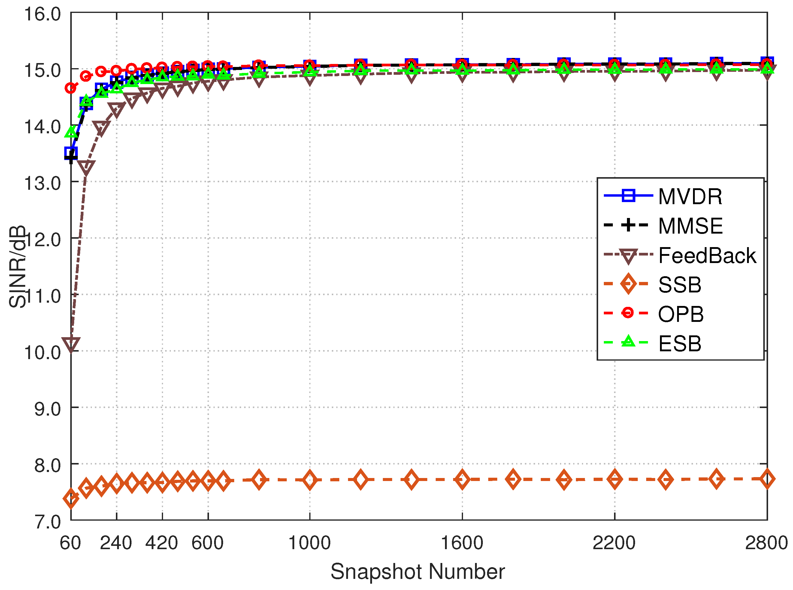
Example 1.
The output SINR versus with the number of snapshots.
In this experiment, the main topic discussed is how the output SINR of the proposed method and other algorithms varies with the snapshots of the echo data. In the scenario set above, the snapshot number of the echo data changes from 60 to 2800. Monte Carlo simulation is performed with 400 trials for each value of snapshot.
In Figure 3, the output SINR of the beamforming methods are given as a function of snapshot number. All performance curves are obtained by averaging over 400 independent Monte Carlo runs at each value of snapshot.
The curves show that all methods converge as the number of snapshot increases. The proposed OPB method converges faster than other methods, and attains to the performance of the optimal beamforming, namely the MVDR and MMSE method. It is meant that the proposed method can effectively receive all the desired signal including the direct path signal and the coherent multipath signal. As discussed in the Section 4, the performance of the proposed OPB method is mainly determined by the DOA estimation accuracy of the incident signal, especially the interference signal. Compared with the results in reference [36], the ESB method cannot suppress the interference well with little snapshots number, when angle difference between the interference and multipath signal is small. The SSB method only receives the direct path signal, while other methods combine the direct signal with the coherent signal, which result in a 3 dB difference between their output SINR. Furthermore, the output SINR gap is about 1.9 dB due to the aperture difference between the whole array and subarray. Therefore, the theoretical SINR difference is about 4.9 dB between the SSB method and other methods. The small angle difference between the interference and multipath signal leads to the great noise power with the high sidelobe of beam pattern, which prevents the SSB method from attaining its theoretical performance.
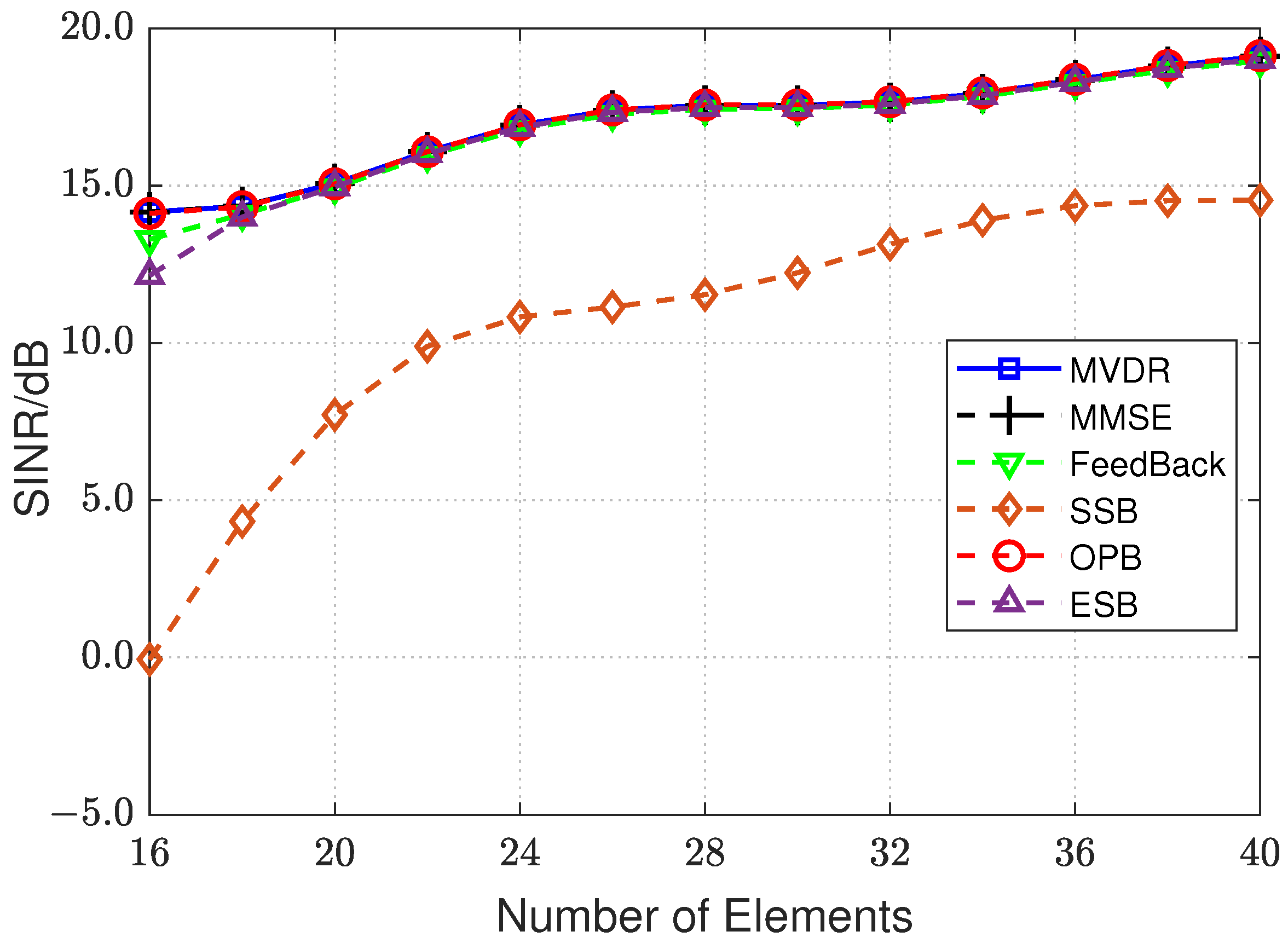
Example 2.
The output SINR versus with the number of elements.
The number of sensors is one of the important influencing factors of beamforming. Therefore, the following experiment studies the sensitivity of the proposed and other above methods to the number of elements. In the scenario set in the beginning of this section, the element number of the array varies from 16 to 40 with other settings unchanged. The snapshot number is chosen as 1600. Monte Carlo simulation is performed with 400 trials for each value of element number.
In Figure 4, the output SINR of the beamforming methods are given versus a different sensor number. All performance curves are obtained by averaging over 400 independent Monte Carlo runs at each value of sensor number. From the simulation result, the performance of all the methods improves with the increase of the number of sensors. However, the ESB and Feedback method can not approach the optimal performance with a small sensor number. But for the proposed method, it is obvious that it is very close to the optimal performance with all sensor numbers. This experiment further verifies the superiority of the proposed OPB method.
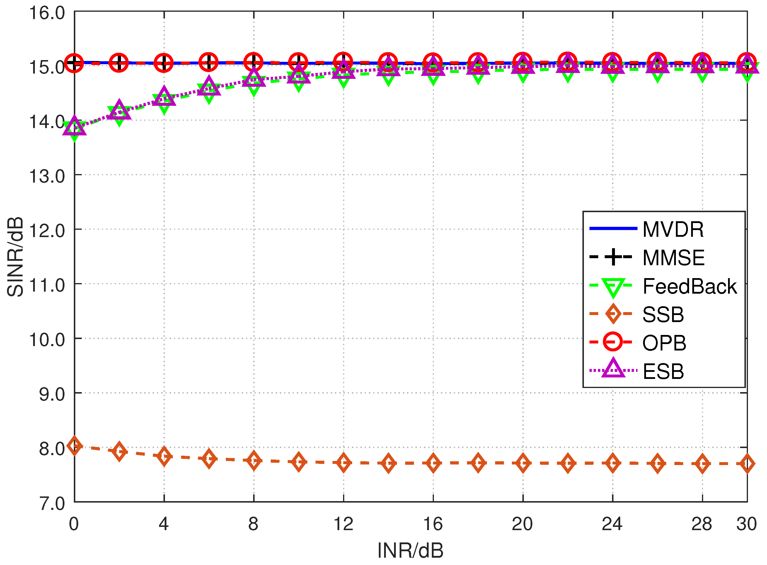
Example 3.
The output SINR versus with the input INR.
In this experiment, the influence of the input INR is studied on the performance of the proposed and other above methods. In the scenario set in the beginning of this section, the input INR varies from 0 dB to 30 dB with other settings unchanged. The snapshot number is set as 1600. Monte Carlo simulation is performed with 400 trials for each value of the input INR.
As shown in 
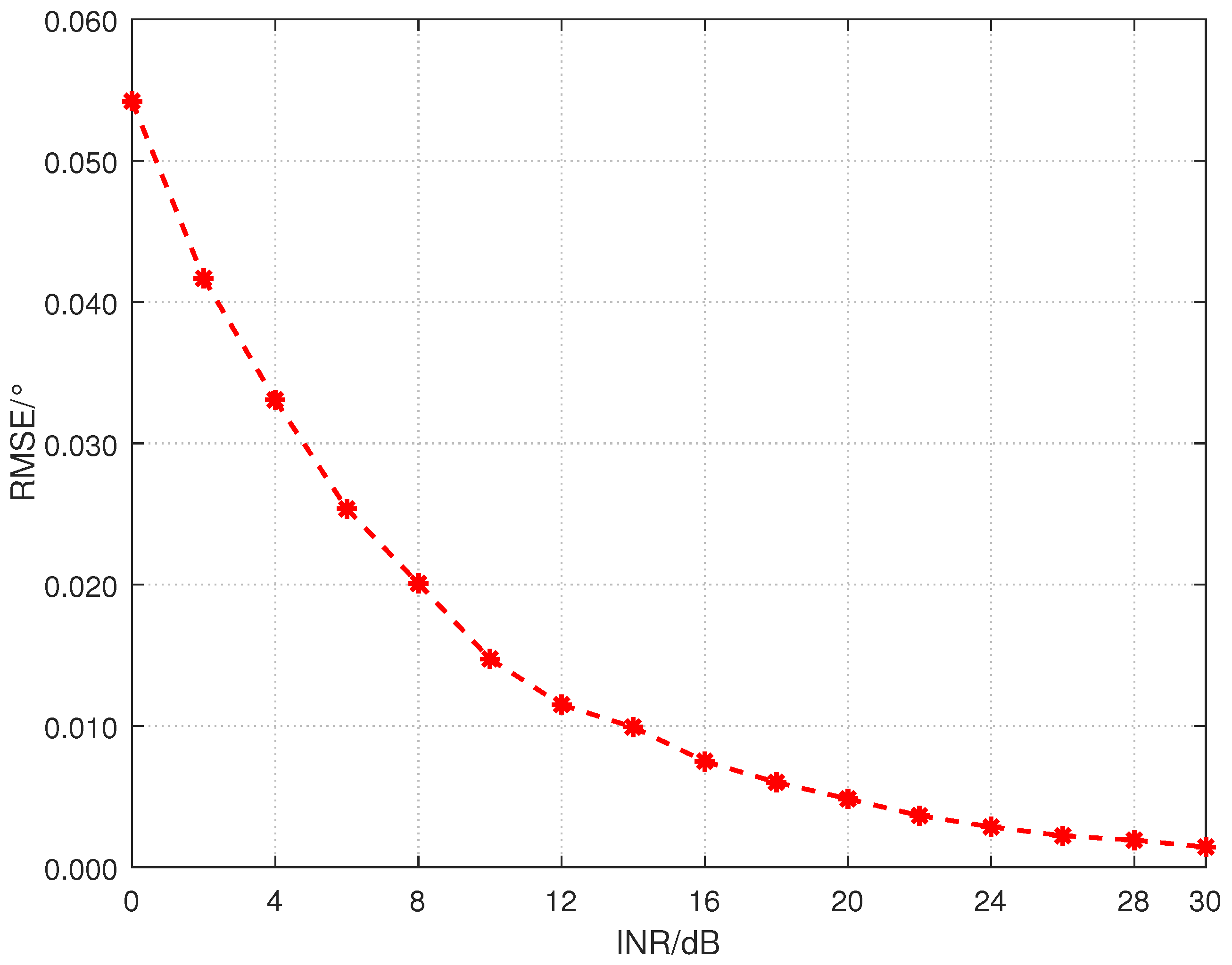
Figure 5, the input INR nearly has no influence on the performance of the proposed OPB method, MVDR and MMSE method. when the input INR is small, the interference space is not the principal of the signal space with the existence of the desired signal, which accounts for the performance degradation of the ESB method. With the increase of the input INR, the more the proportion of interference, the better the ESB method performs. The reason that the proposed OPB method is not affected by the input INR is the DOA estimation accuracy of the interference is enough in the range from 0 dB to 30 dB. The root mean squared error (RMSE) of the interference’s DOA estimation is given versus the input INR in the Figure 6. Although the RMSE is greater with lower INR, the interference perturbation caused by the estimation error is less accordingly. Therefore, the performance of the proposed OPB method is almost unchanged in the given INR range.
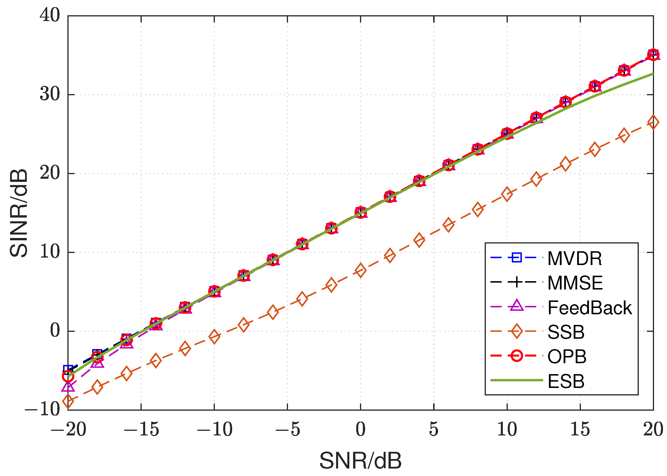
Example 4.
The output SINR versus with the input SNR.
In this experiment, the influence of the input SNR is studied on the performance of the proposed and other above methods. In the scenario set in the beginning of this section, the input SNR varies from −20 dB to 20 dB with other settings unchanged. The snapshot number is also set as 1600.
In Figure 7, the output SINR of the beamforming methods are given versus different input SNRs. All performance curves are obtained by averaging over 400 independent Monte Carlo runs at each value of the input SNR. From the simulation result, we can draw the conclusion that the proposed method has no relationship with the input SNR. But the ESB method suffers from the performance degradation when the input SNR 15 dB, which is for the same reason that accounts for the case with low input INR in the previous experiment. For the Feedback method, the proportion of the desired signal is less in the S-MVDR beamforming output when the input SNR is very low, which leads to its performance degradation of the final output. Although the DOA estimation is seriously degraded with low SNR, and even the DOA of the multipath coherent signal can not be estimated, as analysed in Section 4, the proposed OPB method is not affected by the DOA estimation error of the multipath coherent signal. Simulation results show that the proposed OPB method is more robust for the input INR and SNR than other methods, keeping pace with the ideal optimal beamforming method.

7. Conclusions

In this paper, the problem of coherent signal beamforming is studied in a multipath case. In the presence of irrelevant interference, the proposed oblique projection-based beamformer (OPB) can combine the coherent signals and suppress the interference effectively. The composite steering vector of the multipath coherent signals is extracted by an oblique projection matrix, which is then used to obtain the weight vector with MVDR criteria. Although prior information is required about the angles of incident signals, the performance of the proposed method is robust as long as the angle of the irrelevant interference is estimated accurately, a condition which is satisfied generally. The composite steering vector is obtained without the estimation of the reflection coefficients of multipath signals. Therefore, the computational complexity is reduced greatly. Moreover, the proposed beamformer is more robust and converges to optimal beamformer rapidly without aperture loss.

Author Contributions

Conceptualization, Y.G., Q.L. and L.Z.; methodology, Y.G., Q.L. and J.Z.; software, Y.G. and Q.L.; validation, L.Z., Q.L., J.Z. and Z.C.; writing—original draft preparation, Y.G. and Q.L.; writing—review and editing, L.Z., J.Z. and Z.C. All authors have read and agreed to the published version of the manuscript.

Funding

This work was supported in part by the National Natural Science Foundation of China under Grants 61601343, 61671361, 61871305, 61971329 and 62001062, and in part by the Natural Science Foundation of the Shaanxi Province under Grant 2018JM6054.

Data Availability Statement

Not applicable.

Conflicts of Interest

The authors declare no conflict of interest.

Abbreviations

The following abbreviations are used in this manuscript:
DOAdirection of arrival
radarradio detection and ranging
SARsynthetic aperture radar
SINRsignal to interference plus noise ratio
MVDRminimum variance distortionless response
MMSEminimum mean squared error
SSBspatial smoothing beamforming
ESBeigenspace-based beamforming
MUSICmultiple signal classification
OPBoblique projection-based beamformer
SNRsignal to noise ratio
INRinterference to noise ratio
RMSEroot mean squared error

References

  1. Jing, C.; Niu, X.; Duan, C.; Lu, F.; Di, G.; Yang, X. Sea surface wind speed retrieval from the first Chinese GNSS-R mission: Technique and preliminary results. Remote Sens. 2019, 11, 3013. [Google Scholar] [CrossRef] [Green Version]
  2. Kim, D.; Lee, H.; Jung, H.C.; Hwang, E.; Hossain, F.; Bonnema, M.; Kang, D.H.; Getirana, A. Monitoring river basin development and variation in water resources in transboundary Imjin river in North and South Korea using remote sensing. Remote Sens. 2020, 12, 195. [Google Scholar] [CrossRef] [Green Version]
  3. Shi, W.; Zhang, M.; Zhang, R.; Chen, S.; Zhan, Z. Change detection based on artificial intelligence: State-of-the-art and challenges. Remote Sens. 2020, 12, 1688. [Google Scholar] [CrossRef]
  4. Yasyukevich, Y.; Vasilyev, R.; Ratovsky, K.; Setov, A.; Globa, M.; Syrovatskii, S.; Yasyukevich, A.; Kiselev, A.; Vesnin, A. Small-scale ionospheric irregularities of auroral origin at mid-latitudes during the 22 June 2015 magnetic storm and their effect on GPS positioning. Remote Sens. 2020, 12, 1579. [Google Scholar] [CrossRef]
  5. Xu, Y.G.; Liu, Z.W.; Gong, X.F. Signal Processing of Polarization Sensitive Array; Bejing Institute of Technology Press: Bejing, China, 2013. [Google Scholar]
  6. Johnson, D.H.; Dudgeon, D.E. Array Signal Processing: Concepts and Techniques; Bejing Institute of Technology Press: Bejing, China, 1992. [Google Scholar]
  7. Trees, H. Detection, Estimation, and Modulation Theory, Optimum Array Processing; Publishing House of Electronics Industry: Bejing, China, 2013. [Google Scholar]
  8. Zhou, Z.Z.; Liu, P.; Gu, R.J. Analysis of radar detection under multipath effect. J. Terahertz Sci. Electron. Inf. Technol. 2013, 146, 736–740. [Google Scholar]
  9. Wang, L.J.; Guo, J.M.; Hao, J. The influence of multipath effect on low altitude cruise missile detection in radar. Radar Sci. Technol. 2010, 8, 204–208. [Google Scholar]
  10. Capon, J. High-resolution frequency-wavenumber spectrum analysis. Proc. IEEE 1969, 57, 1408–1418. [Google Scholar] [CrossRef] [Green Version]
  11. Robert, G.L.; Stephen, P.B. Robust minimum variance beamforming. IEEE Trans. Signal Process. 2005, 53, 1684–1696. [Google Scholar]
  12. Wang, Y.L. Adaptive Array Processing; Tsinghua University Publishing House Co., Ltd.: Bejing, China, 2009. [Google Scholar]
  13. Van Trees, H.L. Optimum Array Processing; Wiley-Interscience: Hoboken, NJ, USA, 2001. [Google Scholar]
  14. Widrow, B.; Kenneth, M.; Richard, P.; William, C. Signal cancellation phenomena in adaptive antennas: Causes and cures. IEEE Trans. Antennas Propag. 1982, 30, 469–478. [Google Scholar] [CrossRef] [Green Version]
  15. Chen, B.T.; Xie, Y.J.; Li, X.F. Analysis of echo signals from low altitude radar targets in actual landform. J. Xi’an Jiaotong Univ. 2010, 44, 103–107. [Google Scholar]
  16. Wang, Y.; Gu, J. Research and simulation analysis of radio reflection characteristic over the ocean. Electron. Des. Eng. 2016, 24, 113–115, 119. [Google Scholar]
  17. Shan, T.J.; Kailath, T. Adaptive beamforming for coherent signals and interference. Acoust. Speech Signal Process. IEEE Trans. 1985, 33, 527–536. [Google Scholar] [CrossRef] [Green Version]
  18. Elmaraazey, M. Improved spatial smoothing for beamforming in the presence of correlated arrivals. In Proceedings of the IEEE International Symposium on Circuits Systems, San Diego, CA, USA, 3–6 May 1992. [Google Scholar]
  19. Tang, J.; Peng, Y.N. A new adaptive spatial smoothing method. In Proceedings of the IEEE Antennas and Propagation Society International Symposium, Columbus, OH, USA, 22–27 June 2003; Volume 3, pp. 284–287. [Google Scholar]
  20. Lei, Z.; Wei, L. Robust beamforming for coherent signals based on the spatial-smoothing technique. Signal Process. 2012, 92, 2747–2758. [Google Scholar]
  21. Wang, B.H. Adaptive array with global weighted spatial smoothing. Electron. Lett. 2004, 40, 460–461. [Google Scholar] [CrossRef]
  22. Ding, Q.J.; Wang, Y.L.; Zhang, Y.S.; Chen, H. An adaptive weighted spatial smoothing algorithm utilizing virtual beamforming. J. Electron. Inf. Technol. 2006, 28, 2263–2268. [Google Scholar]
  23. Zhou, W.; Zhang, D.M.; Wu, B.; Zhou, Z.Z. Study on interference suppression for LCMV adaptive array in coherent environment. J. Electron. Inf. Technol. 2007, 29, 1604–1607. [Google Scholar]
  24. Wang, W.C.; Li, L.; Liu, C.J.; Liu, F. Adaptive beamforming method based on linear prediction and spatial smoothing. Aerosp. Electron. Warf. 2009, 25, 50–52. [Google Scholar]
  25. Wang, Y.; Zhao, Z.J.; Liu, X.L. Robust full array beamforming algorithm. Comput. Eng. Appl. 2014, 50, 205–209. [Google Scholar]
  26. Yeh, C.C.; Wang, W.D. Coherent interference suppression by an antenna array of arbitrary geometry. IEEE Trans. Antennas Propag. 1989, 37, 1317–1322. [Google Scholar] [CrossRef]
  27. Lee, T.S.; Lin, T.T. Coherent interference suppression with complementally transformed adaptive beamformer. IEEE Trans. Antennas Propag. 1998, 46, 609–617. [Google Scholar]
  28. Choi, Y.H. Duvall-structure-based fast adaptive beamforming for coherent interference cancellation. IEEE Signal Process. Lett. 2007, 14, 739–741. [Google Scholar] [CrossRef]
  29. Zhao, Y.B.; Zhang, S.H.; Liao, G.S. Application of the Toeplitz technique to ESB adaptive beamforming. J. Xidian Univ. 2000, 27, 682–685, 690. [Google Scholar]
  30. Cao, Y.H.; Zhang, S.H.; Zhao, Y.B. An adaptive beamforming algorithm in the presence of coherent interference. J. Xidian Univ. 2004, 31, 774–776, 790. [Google Scholar]
  31. Wu, X.D.; Zhao, Y.B.; Zhang, S.H.; Dong, M. Height finding of meter-wave radar using improved Toeplitz technique at low-angle environment. J. Electron. Inf. Technol. 2010, 32, 570–574. [Google Scholar] [CrossRef]
  32. Zhao, Y.B.; Shui, P.L. New beamformer for coherent signal reception in the presence of uncorrelated interferences. In Proceedings of the IEEE International Symposium on Microwave, Antenna, Propagation and EMC Technologies for Wireless Communications (MAPE), Beijing, China, 27–29 October 2009. [Google Scholar]
  33. Lei, Y.; Wei, L.; Richard, J.L. Robust beamforming methods for multipath signal reception. Digit. Signal Process. 2010, 20, 379–390. [Google Scholar]
  34. Wu, R.B.; Jing, Y.Q.; Liu, Z.; Xing, Y.; Yang, R. Robust adaptive beamforming algorithm for multiple coherent signals reception. J. Signal Process. 2014, 30, 7. [Google Scholar]
  35. Ding, Y.C.; Liu, C.C.; Zhao, Y.J. Narrowband multipath signal reception beamforming algorithm based on anti-diagonal unit matrix. J. Radars 2015, 4, 192–198. [Google Scholar]
  36. Cheng, W.; Jun, T.; Ying, W. Eigenspace-based beamforming technique for multipath coherent signals reception. Signal Process. 2016, 128, 150–154. [Google Scholar]
  37. Cheng, W.; Jun, T. Feedback beamforming technique for receiving multipath coherent signals. Multidimens. Syst. Signal Process. 2017, 29, 1449–1457. [Google Scholar]
  38. Wang, C.; Tang, J. Blind beamforming technique for reception of multipath coherent signals. IEEE Commun. Lett. 2016, 20, 1453–1456. [Google Scholar] [CrossRef]
  39. Shan, T.J.; Wax, M.; Kailath, T. On spatial smoothing for direction-of-arrival estimation of coherent signals. IEEE Trans. Acoust. Speech Signal Process. 1985, 33, 806–811. [Google Scholar] [CrossRef]
Figure 1. Illustration of Multipath Environment.
Remotesensing 14 05043 g001
Figure 2. Forward Spatial Smoothing.
Remotesensing 14 05043 g002
Figure 3. Output SINR versus the number of snapshots.
Remotesensing 14 05043 g003
Figure 4. Output SINR versus the number of sensors.
Remotesensing 14 05043 g004
Figure 5. Output SINR versus the input INR.
Remotesensing 14 05043 g005
Figure 6. DOA estimation RMSE versus the input INR.
Remotesensing 14 05043 g006
Figure 7. Output SINR versus the input SNR.
Remotesensing 14 05043 g007
Table 1. The Flow of the Proposed OPB.
(1) Receive Data
      The array receives the direct and multipath coherent signal, irrelevant
      interference and noise.
               x ( t ) = i = 0 K ρ i a N ( θ i ) s d ( t ) + j = 1 P a N ( θ j ) s j ( t ) + n N ( t )
(2) Spatial Smoothing
      The averaged subarray covariance matrix is obtained by spatial smoothing.
                                     R f = 1 M m = 1 M R m
(3) DOA Estimation
      MUSIC algorithm is performed for DOA estimation.
                             P m u s i c = 1 a N M + 1 H ( θ ) U ^ N U ^ N H a N M + 1 ( θ )
      The DOA estimation result is Θ ^ = { θ ^ 1 θ ^ 2 θ ^ 3 } .
(4) Construct Oblique Projection Matrix
      Find the closest estimation of the desired angle θ 0 in a given threshold δ
                      θ i = { arg min θ i | θ ^ i θ 0 | & | θ ^ i θ 0 | δ | θ ^ i Θ ^ }
      where δ is determined by the estimation error.
      If θ i is found, remove it from Θ ^ . Otherwise, do nothing with Θ ^ .
      The steering vector matrix B ^ is B ^ = a ( Θ ^ ) = [ a ( θ ^ 1 ) a ( θ ^ 2 ) ] .
      The oblique projection matrix P a ( θ 0 ) / B ^ is constructed
                      P a ( θ 0 ) / B ^ = a ( θ 0 ) a ( θ 0 ) H P B ^ a ( θ 0 ) 1 a ( θ 0 ) H P B ^
(5)Weight Vector
      The weight vector of the proposed OPB algorithm is
                             W ^ O P = U S U S H P a ( θ 0 ) / B ^ H a ( θ 0 )
(6) Beamforming
      The array output after beamforming is
                             z ( t ) = W ^ O P H x ( t )
Publisher’s Note: MDPI stays neutral with regard to jurisdictional claims in published maps and institutional affiliations.

