Article

Prediction of Radar Echo Space-Time Sequence Based on Improving TrajGRU Deep-Learning Model

1
Key Open Laboratory of Atmospheric Sounding, China Meteorological Administration, Chengdu 610225, China
2
College of Atmospheric Sounding, Chengdu University of Information Technology, Chengdu 610225, China
3
Yunnan Atmospheric Sounding Technology Support Center, Kunming 650034, China
*
Author to whom correspondence should be addressed.
Remote Sens. 2022, 14(19), 5042; https://doi.org/10.3390/rs14195042
Submission received: 26 August 2022 / Revised: 30 September 2022 / Accepted: 5 October 2022 / Published: 9 October 2022

Abstract

:
Nowcasting of severe convective precipitation is of great importance in meteorological disaster prevention. Radar echo extrapolation is an effective method for short-term precipitation nowcasting. The traditional radar echo extrapolation methods lack the utilization of radar historical data as well as overlooking the nonlinear motion of small- to medium-sized convective systems in radar echoes. To solve this, we propose a deep-learning model combining CNN and RNN. The model T-UNet proposed in this paper uses an efficient convolutional neural network of UNet architecture with a residual network, where the encoder and decoder networks are connected by nested dense skip paths, while a TrajGRU recurrent neural network is added at each layer, to achieve the perceptual capability of time series. The quantitative statistical evaluation showed that the use of T-UNet could improve the nowcasting skill (CSI score, HSS score) by a maximum of 10.57% and 7.80% over a 60 min prediction cycle. Further evaluation showed that T-UNet also improved the prediction accuracy and prediction performance in the strong echo region.

Graphical Abstract

1. Introduction

Severe convective precipitation can cause secondary disasters such as debris flows and landslides, which have a great impact on economic development and social security. It is extremely difficult to accurately predict severe convective precipitation, because strong convective precipitation has the characteristics of strong locality, rapid development and nonlinear evolution. Observing strong convection processes using weather radar and predicting the development of radar echoes within 0–1 h can improve the accuracy of nowcasting and is an important issue in nowcasting research [1]. The main difficulty in nowcasting is prediction of strong echo regions and understanding of the evolution meteorological echoes, both of which remain to be addressed despite advances in the past few decades [2].
Traditional nowcasting methods are based on numerical weather prediction (NWP) [3]. The model based on NWP is to describe continuous changes in meteorological elements in time and space through complex atmospheric equations, so as to obtain reasonable and accurate forecast results in a few hours to days. With the increasing amount of temporal and spatial information for prediction, high-resolution NWP-based models put forward extremely high requirements on the information extraction capability and processing time of the computer. Therefore, improved prediction accuracy of NWP-based models is limited with the increase in the amount of data; there is still a large room for improvement in short-term nowcasting [4].
With the development of high-resolution weather radar and meteorological satellites, forecast models based on radar echo and cloud image extrapolation are gradually being applied [5]. It can extract features of the moving trend of convection, so as to play a certain role in judging the evolution of convection.
Currently, radar extrapolation methods used for operational applications mainly focus on thunderstorm-based identifying and tracking, as well as automatic extrapolation of forecasts, including the single centroid method, cross-correlation method and optical flow method [6,7,8]. Single centroid methods, such as TITAN (Thunderstorm Identification, Tracking, Analysis and Nowcasting) [9] and SCIT (Storm Cell Identification and Tracking) [10], provide information on convective cell motion and evolution based on convective cell merging and splitting by identifying and tracking groups of convective cells, whereas the forecast accuracy rapidly decreases when echoes are fused and split. The cross-correlation method, such as TREC (Tracking Radar Echoes by Correlation), calculates spatially optimized correlation coefficients for two proximate moments and subsequently creates a fitting relationship for all radar echoes. It can effectively track stratiform cloud and rainfall systems, but for strong convective processes with fast echo changes, the tracking accuracy is significantly reduced. Optical flow methods, such as ROVER (Real-time Optical flow by Variational methods for Echoes of Radar) [11], calculate the optical flow field from continuous time radar echo images, replace the radar echo motion vector field with the optical flow field, and extrapolate radar echo based on a motion vector field to achieve nowcasting. The optical flow method differs from the cross-correlation method in that it is based on changes rather than selected invariant features, but the problem of cumulative error exists in calculating optical flow vector and extrapolation. In general, these methods only infer the echo position of the next moment from the radar echo images of a few moments earlier, as well as ignoring the motion nonlinearity of small- and medium-scale convective system in the radar echoes under actual conditions; therefore, there are limitations of underutilization of historical radar data and short extrapolation time [12].
Artificial-intelligence technology represented by deep learning with the ability to analyze, associate, remember, learn and infer uncertainty problems has made remarkable progress in the fields of image recognition [13,14,15], image segmentation [16,17,18], natural language processing [19,20,21]. Unlike the traditional approach, deep-learning methods have the ability to learn from massive amounts of data, so as to mine the internal characteristics and physical laws of data. They are widely used to establish complex nonlinear models [22].
In recent years, deep-learning technology has been introduced into meteorological nowcasting and achieved excellent application results. Precipitation nowcasting is a sequence prediction problem based on time and space [23]. To achieve satisfactory results in extrapolation, it is necessary to fully consider the temporal features between continuous time images and the spatial motion features in the images at the same time, which is in-line with the basic characteristics of LSTM-RNN (long short-term memory-recurrent neural network) in deep-learning networks [24]. Shi et al. [25] proposed that LSTM cells with convolution layers make up RNN (ConvLSTM), which can extract spatial characteristics by convolution operation compared to the full connection used by a fully connected LSTM in transfer. As the first attempt of precipitation prediction based on deep learning, the accuracy of ConvLSTM in precipitation nowcasting is significantly improved compared with fully connected LSTM and optical flow methods. A tossed stone causes a thousand ripples; a large number of studies based on ConvLSTM have been proposed [26]. Shi et al. continued to propose a TrajGRU model which can learn from optical flow [27]. On the basis of inheriting the good sensitivity of a temporal convolution neural network to temporal and spatial characteristics, it can learn from the optical flow movement and simulate the real movement of clouds in nature to improve the performance of model extrapolation.
In the above RNN-based model, CNN (convolutional neural network) also plays an important role. CNN can effectively extract image features and map them on the label image [28]. UNeT is a classic full convolution neural network structure which includes down sampling and up sampling [29]. A subsequent improvement of UNet was also implemented to fill its hollow structure, connecting the semantic gap between encoder and decoder feature mappings. This nested UNet is called UNet++ [30]. At present, a UNet-based model is mostly used in the field of image segmentation, mainly in the recognition and segmentation of medical images. Researchers view precipitation nowcasting as an image-to-image conversion problem and use UNet-based structured convolutional neural networks for forecasting purposes, which is a data-driven short-time precipitation nowcasting model that utilizes none of the atmospheric and physical models [31]. Ayzel et al. proposed a precipitation prediction model based on UNet which is comparable to the traditional optical flow method [32]. Nie et al. [33] proposed SelfAtt-UNet based on the UNet network architecture. SelfAtt-UNet introduces a self-attention mechanism on top of UNet so that it can focus on tracking changes in the most influential regions of the radar echo.
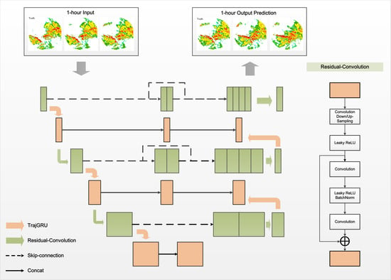
In this paper, a model combining CNN and RNN is proposed to better capture spatial and temporal features. The model is based on a UNet backbone with residual networks, with the addition of TrajGRU in each layer, constituting a new architecture, T-UNet. In addition, the nested dense skip connections are redesigned with the aim of reducing the semantic gap between the feature mappings of the encoder and decoder sub-networks to obtain extra spatio-temporal extraction capability for more accurate echo inference for precipitation nowcasting. The T-UNet model proposed in this paper is a new end-to-end deep network. Compared with other networks, T-UNet nests the recurrent structure of RNN in a complete convolutional network, while extending the ordinary convolution into a residual network. By combining the CNN structure with the RNN structure, the spatio-temporal features in continuous radar echo maps are better captured for more accurate prediction.
The organization of this article is as follows. Section 2 provides a brief overview of the research on nowcasting of precipitation using CNN-based and RNN-based models. In Section 3, the detailed structure of T-UNet is described. Section 4 experimentally evaluates T-UNet against other models. Finally, a summary and concluding comments are presented in Section 5.

2. Application of CNN-Based and RNN-Based Models in Precipitation Nowcasting

The basic idea of radar extrapolation for precipitation nowcasting is to track the movement of echoes based on radar observations, extrapolate the position of echoes at the future time, and invert the precipitation distribution in the future period through the Z–R relationship [34].
Two types of deep-learning models that are mainly used for precipitation nowcasting are methods of predicting sequence values between sequences based on RNN and methods of extracting the main features of sequences based on CNN.
Both ConvLSTM and TrajGRU are RNN-based precipitation nowcasting models that have been proven to have excellent performance, in which the latter can better learn the structure and weights of location change, and based on GRU has lower memory requirements than LSTM, saving a lot of computing time [35]. Wang et al. [36] proposed a new end-to-end structure, PredRNN, which allows cross-layer interaction of cells belonging to different LSTMSs, and designed a new spatiotemporal LSTM (ST-LSTM) unit, which memorizes spatial and temporal characteristics in a single memory unit and transfers memory at the vertical and horizontal levels. In the test including the radar dataset, PredRNN achieves better prediction results than ConvLSTM. The E3d-LSTM model proposed by Wang et al. [37] integrates 3D convolution into LSTM, changes the update gate of LSTM, and adds a self-attention module, which enables the network to have better recognition of the early activity of radar echoes, thus combining the two networks at a deeper mechanism level.
With its excellent spatial extraction ability, UNet is widely used as a backbone based on a full CNN model. Trebing et al. [38] added attention modules to UNet and replaced traditional convolution with depthwise-separable convolution. The results after the radar echo extrapolation experiment show that the SmaAt-UNet proposed by the author can reduce the number of parameters to 1/4 of the original one at the expense of a small number of indicators. Since UNet has a flexible structure, Pan et al. [39] proposed a new model named FURENet, using UNet as a backbone network, which met the purpose of inputting multivariable information. The polarimetric radar parameters K D P and Z D R are input into the model to improve the accuracy of precipitation nowcasting.
Convolutional neural networks enable feature learning through image filters by treating the input grid weather elements as images, which sufficiently capture the spatial structure of the correlation, but lack the ability to handle sequential data and are only suitable for ‘fixed-length’ data. A recurrent neural network, which is often used in natural language processing, has an autoregressive structure that allows for flexible processing of sequential data and effective learning in the temporal dimension, with the disadvantage that, like the multilayer perceptron, the input features can only be characterized by a one-dimensional vector, thus losing the inherent spatial characteristics of the lattice data, and the learning ability is relatively poor. Combining the above two models in different forms, which can learn both spatial and temporal features, is more suitable for solving the problem of precipitation nowcasting. In the following, the specific construction of T-UNet combining CNN and RNN structures will be discussed, as well as its performance being verified on the dataset.

3. T-UNet Model

3.1. UNet

The T-UNet model is based on the UNet architecture. As shown in Figure 1, the backbone of UNet (the black down-sampling and up-sampling component in Figure 1a) is composed of three encoding–decoding layers connected by skip connection in a U-shape. The redesigned skip paths (shown in red) that connect the additional up-sampling and RNN modules to UNet distinguish the model from UNet. The encoding layer is represented by the blue module, while the forecasting layer is represented by the orange module. In each down-sampling layer of the encoder, the size of each frame is halved and the number of channels is doubled through the convolution layer to realize down-sampling and extract features from the image sequence. Similarly, the size of the frame is doubled and the number of channels is halved by transposing convolution layers in the up-sampling decoding layer. Unlike the encoding layer, the input of the decoding layer is fused with the output of the previous layer of the same dense block and with the corresponding up-sampling output of the lower dense block, namely, all previous feature mappings are gathered and delivered to the current node, while the output of the decoding layer is used to achieve sequence prediction with TrajGRU.
The RNN layers are inserted after the convolution to form the down-sampling layer; on the contrary, the deconvolution is inserted after the RNN layers to form the up-sampling layer. In addition, as shown in Figure 1b, extra convolutional operations are added with residual connections in all convolutional layers. The reason for this inverted structure is to make it easier to connect CNN and RNN layers with their own layers at the same level, thus enabling a higher level state to guide lower level state updates. Skip connections play an important role in T-UNet. Down-sampling feature maps are concatenated to the up-sampling layer, which is called long skip connections. The purpose of long skip connections is to reduce the loss of spatial information caused by down-sampling process. The concatenation method makes the up-sampling recovered feature map contain more low-level semantic information, so as to obtain more accurate results. T-UNet consists of consecutive CNN layers and RNN layers with a certain network depth. Appropriate depths are beneficial to regularization; on the contrary, it may lead to over fitting or under fitting. Adding additional short connections to form ResNet in each CNN layer may alleviate the problem of gradient vanishing without changing the network depth. Each convolution layer is modified as shown in the Figure 1b, short connections represent identity mapping, that is, the features of shallow networks are copied to form new features with residuals. The feature mapping after introducing the residual is more sensitive to changes in the output; the network will converge steadily without considering vanishing of the gradient. More details of the model can be found in Appendix A.

3.2. TrajGRU

ConvGRU and other convolution time-series networks have the disadvantage of having a fixed connection structure and parameters for each location in the image when using models to capture spatiotemporal correlation features. In other words, for a particular input, convolution is actually a process of filtering with a locally fixed filter. Different from ConvGRU, the current input and previous hidden states are used by TrajGRU to create a flow field, which is subsequently warped via bilinear sampling (see Figure 2).
The main formulas of TrajGRU are as follows; here, ‘*’ is the convolution operation and ‘∘’ is the Hadamard product:
U t , V t = γ X t , H t 1
z t = σ W x z * X t + l = 1 L W h z l * warp H t 1 , U t , l , V t , l
R t = σ W x r * X t + l = 1 L W h r l * warp H t 1 , U t , l , V t , l
H t = f W x h * X t + R t l = 1 L W h h l * warp H t 1 , U t , l , V t , l
H t = 1 z t H t + z t H t 1
In the above equations, Z t , R t , H t , H t R C h × H × W represent the update gate, reset gate, new information, and memory state. X t R C i × H × W is the input, and σ , f stands for the activation, which are sigmoid and LeakyReLU, respectively. Different from ConvGRU, L means the number of local links; W h z l , W h r l , W h h l are the projection channels weight through 1 ∗ 1 convolutions; warp function is a bilinear interpolation and γ is the “structure generation network” which generates the index X t , H t 1 of the optical flow component. Since X t , H t 1 is a float type and decimals may occur, bilinear interpolation methods are required to find their corresponding eigenvalues. Whenever new inputs arrive, the reset gate determines how the new input information is combined with the previous memory. The update gate is used to control the extent to which the state information of the previous time is brought into the current state; that is, the update gate helps the model decide how much information from the past should be transfered to the future. In short, it is used to update the memory.
Compared with the calculation formula of ConvGRU, the TrajGRU model takes one more step to generate the optical flow component index, followed by the hidden state processing in the last moment. For ConvGRU, each position on the convolution resulting feature graph is fixed to the connection position and weight on the previous feature graph, whereas TrajGRU is not fixed, it is the L dynamically computed connection positions and their weights in the formula above.

3.3. Compared Models

The optical-flow method: Optical flow refers to the change in gray value between pixel points on a sequential frame, namely, the instantaneous velocity of an object while it is in motion. By investigating the optical-flow field of the image sequence, the optical-flow method uses the difference between the optical-flow information of the moving object in the image and that of the background to determine the position of the moving object and, thus, detect the moving target.The optical flow method can be divided into dense optical flow and sparse optical flow according to the sparsity of the two-dimensional vectors in the optical wave field [40]. The dense optical-flow method calculates the instantaneous velocity of all pixels in an image with high accuracy and high computational power, while the sparse optical-flow method calculates the instantaneous velocity of specific feature pixels with lower accuracy than the dense optical flow method, but with less computational power. In this paper, the dense optical flow method is used as the traditional non-artificial-intelligence algorithm for comparison.
SmaAtUNet: The SmaAtUNet model proposed by Kevin Trebing et al. [38] introduces two innovative improvements to UNet that demonstrate fully convolutional neural networks can also have advanced performance in radar echo extrapolation. First, the convolutional block-attention module (CBAM) is added to the coding layer. This module mainly consists of channel attention and spatial attention, which is applied initially to the channel of the image and subsequently to the spatial dimension. The authors use the convolutional block-attention module to identify important features across channels and spatial regions of the image. Second, the authors replace the original convolutional layer with a deep separable convolution (DSC), which splits the regular convolution operation into two separate operations: deep convolution followed by point-by-point convolution. This is able to reduce the parameters and the number of operations.
TrajGRU: Considering the shortcoming that TrajGRU lacks spatial features, Shi et al. [27] implemented the structure of encoding-forcasting to extend the TrajGRU unit. The encoding-forcasting structure first encodes the input image as the hidden state of a three-layer RNN, then uses another three-layer RNN to generate the corresponding predicted image based on the previous hidden layer.

4. Dataset and Experiments Design

Quality-control information and details about this dataset are described at length in Fiolleau and Roca (2013b). The identifying and tracking algorithm used here is the tracking of an organized convection algorithm through the 3D segmentation (TOOCAN) approach (Fiolleau and Roca 2013a). The TOOCAN method can be seen as an extension of the detect-and-spread technique.

4.1. Dataset

The HKO-7 dataset, developed by the Hong Kong Observatory, provides radar constant altitude plan position indicator (CAPPI) reflectivity images updated every 6 min, at a covering area of 512 km × 512 km area with 2 km altitude centered in Hong Kong. The radar reflectivity factor is linearly converted to the pixel value of the image range from 0 to 255 using the following formula:
pixel = 255 × d B Z + 10 70 + 0.5
The radar echo image is based on reflectivity conversion, in which the value of the pixel points in the image corresponds to the radar echo intensity. The higher the reflectivity value, the stronger the radar echo intensity, and the larger the value of the corresponding pixel points, the higher the probability of precipitation. Due to the requirement of computational speed for the model, image resolutions of 480 × 480 in the original dataset are scaled to 256 × 256 by resampling regional pixels.
The HKO-7 dataset was selected for the period of January 2009 through December 2015, covering 993 precipitation events. A total of 812 of 993 days with precipitation were screened for training, 50 days for validation, and 131 days for testing. The radar reflectivity data can be converted to rainfall intensity values based on the Z–R relationship: dBZ = 10 log a + 10 b log R , parameters a, b are calculated separately as 58.53 and 1.56 by linear regression. Based on the six thresholds [0, 0.5], [0.5, 2.0], [2.0, 5.0], [5.0, 10.0], [10.0, 30.0] and [30.0, ∞) of millimeter rainfall per hour, the 993-day precipitation is visualized as follows, where x stands for rainfall intensity values (mm/h):
As shown in Figure 3, precipitation is unevenly distributed in the dataset, with slight precipitation accounting for 90 percent.

4.2. Experimental Design

The approach in the experiment is to predict the reflectivity in the next hour through the radar reflectivity echo map within one hour. As shown in Figure 4, ten consecutive echo maps were fed into the model for training and testing, subsequently outputting ten successive frames of the future maps predicted by the model.
As for the loss function of the model, the weighted B-MSE and B-MAE functions proposed by Shi [27] are used. Considering the uneven distribution of precipitation in the dataset, B-MSE and B-MAE are improved functions to increase the weight of the loss function for pixels with high precipitation on the basis of conventional MSE and MAE, respectively, which can improve the accuracy of the nowcasting of heavy precipitation and lead to more practical significance. The loss function is obtained by weighting the sum of B-MSE and B-MAE1:1 with the following equation:
LOSS = 1 N n = 1 N i = 1 256 j = 1 256 w n , i , j x n , i , j x ^ n , i , j 2 + 1 N n = 1 N i = 1 256 j = 1 256 w n , i , j x n , i , j x ^ n , i , j
The evaluation metric of forecast accuracy in meteorology mainly adopts the idea of binary classification. A confusion matrix is constructed based on the relationship between each grid point and the rain threshold value in the image, which includes TP (prediction = 1, truth = 1), FN (prediction = 0, truth = 1), FP (prediction = 1, truth = 0), and TN (prediction = 0, truth = 0). Five thresholds are mainly used, 0.5, 2, 5, 10, and 30, whose ranges represent light rain, light-to-moderate rain, moderate rain, moderate-to-heavy rain, and heavy rain. Using the above methods, the evaluation metric was defined as follows:
CSI = TP TP + FN + FP
HSS = TP × TN FN × FP ( TP + FN ) ( FN + TN ) + ( TP + FP ) ( FP + TN )
CSI reflects the relative accuracy of prediction; HSS can penalize false or missed alarm and give the expected score of 0 to random and constant predictions. CSI and HSS vary from 0 to 1. The higher their values, the better the predictive performance of the model [41].
The optical-flow method, encoder-forecaster TrajGRU and SmaAt-UNet are adopted as baselines to evaluate the performance of T-UNet and other precipitation prediction models. In the training section, the batch size is set to 4, with a total of 100,000 iterations. The learning scheduler used is ReduceLROnPlateau, which reduces the learning rate to 50% when the loss of the validation set is no longer reduced for six consecutive iterations. The initial learning rate is set to 0.0001, kernel size is set to 3, and Adam is used as optimizer. All models and algorithms are implemented on Pytorch and run in NVIDIA Tesla P40 with 24 GB of RAM.

5. Results

After training the models, we selected the one with the lowest loss function in each model validation set for testing. The metrics used are described in Section 4.2. Table 1 presents the quantitative results of the final prediction results of each model under the regression evaluation metrics, while Table 2 demonstrates the meteorological metric scores of each model under different precipitation thresholds. It can be seen that, among the various loss functions, the results of T-UNet are superior to the other models, proving its better predictive ability. The CSI and HSS scores of SmaAt-UNet show a substantial decline at thresholds greater than 5 mm/h and especially at thresholds greater than 30 mm/h, showing its poor prediction ability for heavy rainfall prediction, which is also reflected in the B-MSE and B-MAE. It is worth mentioning that the MSE and MAE of SmaAt-UNet do not deviate much compared with other models, indicating that the balanced loss function is more effective in reflecting the ability to predict heavy precipitation, consistent with the needs of practical applications. T-UNet performs best in both CSI and HSS scores with different thresholds, signifying that it maintains good details in both clear-rainy forecast and storm predictions, thus reflecting the actual conditions in the rain area.
In the experiment, ten consecutive radar echo maps are fed into the model to obtain the prediction results for the next 60 min; in other words, the historical 1 h data is used to predict the future 1 h echo data. Two representative cases were selected from the test set, and the extrapolation results of each model were further evaluated using visualization analysis and prediction metrics, so as to assess the accuracy of the extrapolation results of T-UNet.
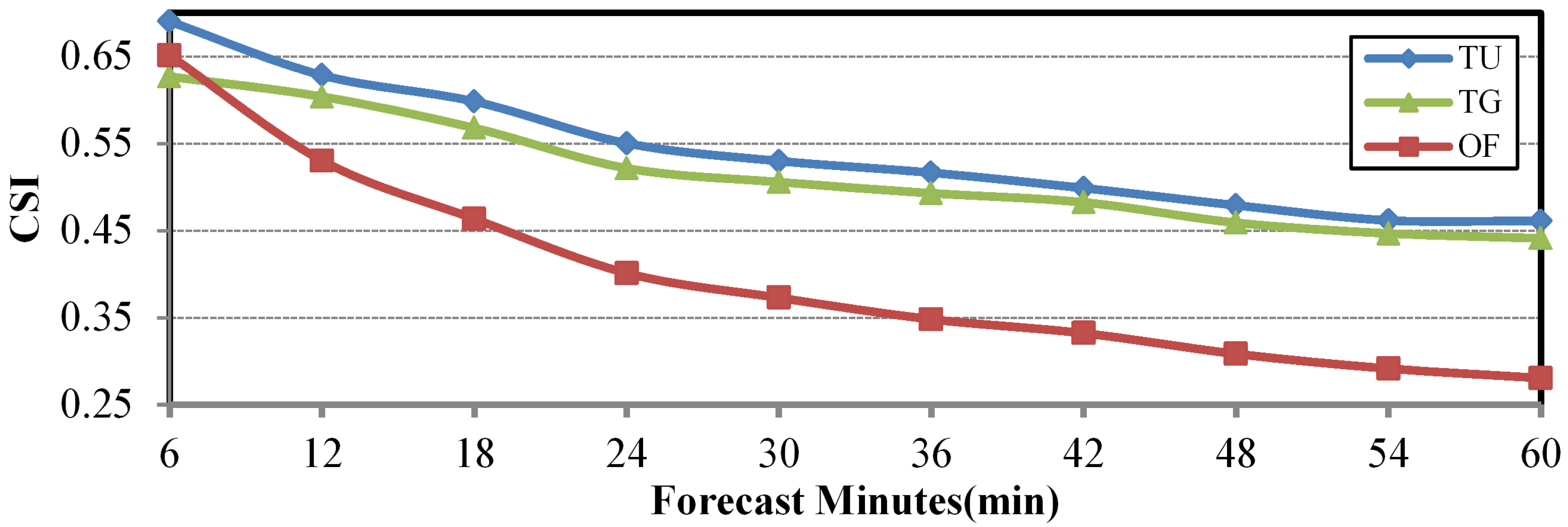
The first case we selected happened from 4:12–6:12 UTC on 23 May 2015, which coincided with the issuance of a yellow rainstorm warning by the Hong Kong Observatory, when the radar captured the gradual merging of the squall line with the storm monomer to form a larger linear convective system. In Figure 5, the ground truth used for the evaluation and the outputs of the four experiments, optical flow method (OF), SmaAt-UNet (SU), TrajGRU (TG) and T-UNet (TU), are shown in turn. For convenience of display, we present a radar echo map every 12 min. In OF, although the optical flow method maintains a high resolution, it is completely unable to predict the evolution of the squall line. It can be demonstrated that, in individual cases of rapidly changing thunderstorms, the optical-flow method is unable to predict the area where the strong echo region is located. The shape and intensity of the echoes in SU are barely satisfactory, and its premature conflation of squall lines with thunderstorm monoliths again loses considerable detail. It can be seen from the prediction plots of TG and TU that T-UNet retains some details in prediction. As shown in the black box, the contours of the strong echo region in the box plot are reflected in the TU. In addition, we selected the CSI and HSS scores of each model in forecast time for precipitation greater than 10 mm/h (the 10 mm/h threshold is commonly used to identify strong convection [9]). SmaAt-UNet is not included in the figure due to its low performance in this section. As shown in Figure 6, the CSI score of T-UNet gradually decreased from 0.69 to 0.46 as the prediction time increased, but the score remained higher than that of TrajGRU throughout the process, as the same was true for the HSS score. Among them, the mean CSI score of T-UNet improved by 5.17% and the mean HSS score improved by 3.92% compared to TrajGRU during this period.
Another case is shown in Figure 7 which occurred at 5:36–7:36 UTC, 4 October 2015, when a super typhoon Mujigae made landfall near Zhanjiang City, Guangdong Province. Radar echo maps from the Hong Kong Observatory captured the evolution of the Mujigae’s outer rain belt. The Mujigae brings strong gale and cyclones which make the rain area more unpredictable, greatly enhancing the difficulty of precipitation nowcasting. As can be seen from Figure 7, T-UNet and TrajGRU can predict the approximate location of the strong echoes more accurately in the first thirty minutes. After thirty minutes, both models lose some echo details, but compared to TrajGRU, T-UNet is still able to maintain the accuracy of predicting the strong echo region, as can be seen from the black box. Admittedly, as the prediction time increases, the prediction details are lost; that is, multiple echo regions are combined into one whole echo in the predicted image, causing the predicted echo intensity larger than the ground truth value, which needs to be improved in future experiments. From the perspective of quantitative assessment (see Figure 8), none of the models involved in the experiment performed as well as Case 1 in Case 2, which was caused by the more rapid and irregular changes in the strong gale weather process. The CSI and HSS scores of T-UNet in the first 30 min did not widen the gap with TG, which became more sufficient in the last 30 min. Over the prediction time, the CSI and HSS of T-UNET decreased from 0.63 and 0.75 to 0.30 and 0.40, respectively, scoring consistently higher than TrajGRU during this process. In terms of average score, the CSI and HSS of T-UNet improved by 6.86% and 7.37%, respectively. Overall, the prediction performance of T-UNet within 60 min in case 2 is better than that of TrajGRU.

6. Conclusions

In this study, a novel radar echo extrapolation model based on CNN and RNN is proposed, named T-UNet. The model uses the UNet structure as a framework and redesigns the dense jump connections to reduce the semantic gap between feature mappings with different levels of upsampling and downsampling. TrajGRU is introduced into UNet for forming T-UNet to learn spatio-temporal features. In the experiments, the prediction results of T-UNet were compared with those of the CNN model SmaAt-UNet, the RNN model TrajGRU, and the dense optical-flow method on the HKO-7 dataset. The following main conclusions are obtained from the evaluation results:
  • Visual analysis results from two cases show that T-UNet can relatively effectively preserve the spatio-temporal characteristics of radar images in prediction; particularly, the details of strong echoes are closer to the ground truth.
  • The results obtained from the test set show that T-UNet improves by 9.6% and 7.05% in terms of B-MSE and B-MAE compared to TrajGRU, and similarly improve by 9.03% and 7.21% in terms of MSE and MAE. In addition, T-UNet performs better than TrajGRU at different thresholds for the common scoring functions CSI and HSS in meteorology, CSI has a maximum improvement by 10.57% at thresholds greater than 30 mm/h, and HSS also reaches a maximum improvement by 7.80% at thresholds greater than 30 mm/h. These numerical results show that T-UNet has higher accuracy than TrajGRU in the prediction of precipitation proximity and better ability in the prediction of strong echoes.
Although T-UNet improves the accuracy of precipitation nowcasting, like other deep-learning models, it also faces the situation that too much detail is lost in the late prediction stage, and the resolution cannot be maintained as the optical flow method, resulting in a significant decrease.
In future experiments, information from multiple input variables will be added to the model to make predictions, such as variables V, K D P , Z D R and C C of polarimetric radar [42]. These variables can provide additional critical microphysical and dynamic evolution information of convective storms and help to fully reflect the spatio-temporal characteristics of convective processes.

Author Contributions

Conceptualization, Q.Z., H.L., T.Z. and F.Z.; methodology, Q.Z., H.L., J.H. and F.Z.; software, Q.Z., H.L. and H.W.; validation, Q.Z.; formal analysis, Q.Z., H.L. and Z.Q.; investigation, F.Z. and J.H; resources, Q.Z. and H.W.; data curation, Q.Z.; writing—original draft preparation, H.L.; writing—review and editing, Q.Z., H.L. and H.W.; visualization, Z.Q. and B.S.; supervision, F.Z.; project administration, Q.Z. and Q.Y.; funding acquisition, Q.Z. All authors have read and agreed to the published version of the manuscript.

Funding

This research was funded by the Key R&D Program of Yunnan Provincial Department of Science and Technology (202203AC100021), the Fund of Key Laboratory of Atmosphere Sounding, CMA (2021KLAS01Z), the National Natural Science Foundation of China (U20B2061), Special Funds for the Central Government to Guide Local Technological Development (2020ZYD051), the Open Grants of the State Key Laboratory of Severe Weather (2020LASW-B11), Project of the Sichuan Department of Science and Technology (2022YFS0541).

Data Availability Statement

The HKO-7 dataset used in this study is from the Hong Kong Observatory.

Acknowledgments

The author thank the reviewers for their constructive comments and editorial suggestions that significantly improved the quality of this paper.

Conflicts of Interest

The authors declare no conflict of interest.

Abbreviations

The following abbreviations are used in this manuscript:
NWPNumerical weather prediction
TITANThunderstorm Identification, Tracking, Analysis and Nowcasting
SCITStorm Cell Identification and Tracking
TRECTracking Radar Echoes by Correlation
ROVERReal-time Optical flow by Variational methods for Echoes of Radar
LSTMLong short term memory
RNNRecurrent neural networks
GRUGated Recurrent Unit
ConvLSTMConvolutional LSTM
TrajGRUTrajectory GRU
CNNConvolutional neural networks
SmaAt-UNetSmall AttenStion-UNet
CSICritical success index
HSSHeidke skill score
MSEMean square error
MAEMean absolute error

Appendix A

Appendix A.1

Using U-Net as the backbone of T-UNet, additional convolutional operations are added using residual connections as well as redesigned jump connections to enhance the capacity of the model, and TrajGRU is added at each layer to achieve spatio-temporal awareness capability. The detailed settings of the model hyperparameters and training procedure are shown in Table A1. The parameter L of TrajGRU in the network structure represents the number of links in the state-to-state transition. Kernel size, stride and padding represent of height and width in two dimensions.
Table A1. The details of the T-UNet.
ObjetcsSettings
Basic layers3
Numbers of long skip-connection7
Convolutional filtersFirst layer64
Second layer128
Third layer256
Down/Up-samplingKernel size4 × 4
Stride2 × 2
Padding1 × 1
Residual networkKernel size3 × 3
Stride1 × 1
Padding1 × 1
TrajGRUKernel size3 × 3
Stride1 × 1
Padding1 × 1
L15

Appendix A.2

Table A2. The detail of the SmaAt-UNet.
ObjetcsSettings
Basic layers5
Numbers of long skip-connection4
Reduction ratio of CBAM16
Convolutional filtersFirst layer64
Second layer128
Third layer256
Third layer512
Third layer512
Down/Up-samplingKernel size3 × 3
Stride1 × 1
Padding1 × 1

Appendix A.3

Table A3. The detail of the TrajGRU.
ObjetcsSettings
Basic layers3
Reduction ratio of CBAM16
Convolutional filtersFirst layer64
Second layer192
Third layer192
Convolution in RNN unitKernel size3 × 3
Stride1 × 1
Padding1 × 1

References

  1. Seed, A. A dynamic and spatial scaling approach to advection forecasting. J. Appl. Meteorol. 2003, 42, 381–388. [Google Scholar] [CrossRef]
  2. Wilson, J.W.; Crook, N.A.; Mueller, C.K.; Sun, J.; Dixon, M. Nowcasting thunderstorms: A status report. Bull. Am. Meteorol. Soc. 1998, 79, 2079–2100. [Google Scholar] [CrossRef]
  3. Bauer, P.; Thorpe, A.; Brunet, G. The quiet revolution of numerical weather prediction. Nature 2015, 525, 47–55. [Google Scholar] [CrossRef] [PubMed]
  4. Mehrkanoon, S. Deep shared representation learning for weather elements forecasting. Knowl.-Based Syst. 2019, 179, 120–128. [Google Scholar] [CrossRef]
  5. Reyniers, M. Quantitative Precipitation Forecasts Based on Radar Observations: Principles, Algorithms and Operational Systems; Institut Royal Météorologique de Belgique Brussel: Brussel, Belgium, 2008. [Google Scholar]
  6. Kawakatsu, H. Centroid single force inversion of seismic waves generated by landslides. J. Geophys. Res. Solid Earth 1989, 94, 12363–12374. [Google Scholar] [CrossRef]
  7. Cireşan, D.C.; Giusti, A.; Gambardella, L.M.; Schmidhuber, J. Mitosis detection in breast cancer histology images with deep neural networks. In Proceedings of the International Conference on Medical Image Computing and Computer-Assisted Intervention, Nagoya, Japan, 22–26 September 2013; Springer: Berlin/Heidelberg, Germany, 2013; pp. 411–418. [Google Scholar]
  8. Lucas, B.D.; Kanade, T. An Iterative Image Registration Technique with an Application to Stereo Vision. In Proceedings of the IJCAI’81: 7th International Joint Conference on Artificial Intelligence, Vancouver, BC, Canada, 24—28 August 1981; Volume 81. [Google Scholar]
  9. Dixon, M.; Wiener, G. TITAN: Thunderstorm identification, tracking, analysis, and nowcasting—A radar-based methodology. J. Atmos. Ocean. Technol. 1993, 10, 785–797. [Google Scholar] [CrossRef]
  10. Johnson, J.; MacKeen, P.L.; Witt, A.; Mitchell, E.D.W.; Stumpf, G.J.; Eilts, M.D.; Thomas, K.W. The storm cell identification and tracking algorithm: An enhanced WSR-88D algorithm. Weather Forecast. 1998, 13, 263–276. [Google Scholar] [CrossRef]
  11. Woo, W.; Wong, W. Application of optical flow techniques to rainfall nowcasting. In Proceedings of the 27th Conference on Severe Local Storms, Madison, WI, USA, 3–7 November 2014. [Google Scholar]
  12. Gultepe, I.; Sharman, R.; Williams, P.D.; Zhou, B.; Ellrod, G.; Minnis, P.; Trier, S.; Griffin, S.; Yum, S.; Gharabaghi, B.; et al. A review of high impact weather for aviation meteorology. Pure Appl. Geophys. 2019, 176, 1869–1921. [Google Scholar] [CrossRef]
  13. Simonyan, K.; Zisserman, A. Very deep convolutional networks for large-scale image recognition. arXiv 2014, arXiv:1409.1556. [Google Scholar]
  14. Russakovsky, O.; Deng, J.; Su, H.; Krause, J.; Satheesh, S.; Ma, S.; Huang, Z.; Karpathy, A.; Khosla, A.; Bernstein, M.; et al. Imagenet large scale visual recognition challenge. Int. J. Comput. Vis. 2015, 115, 211–252. [Google Scholar] [CrossRef] [Green Version]
  15. Szegedy, C.; Ioffe, S.; Vanhoucke, V.; Alemi, A.A. Inception-v4, inception-resnet and the impact of residual connections on learning. In Proceedings of the Thirty-First AAAI Conference on Artificial Intelligence, San Francisco, CA, USA, 4–9 February 2017. [Google Scholar]
  16. Chen, L.C.; Papandreou, G.; Kokkinos, I.; Murphy, K.; Yuille, A.L. Deeplab: Semantic image segmentation with deep convolutional nets, atrous convolution, and fully connected crfs. IEEE Trans. Pattern Anal. Mach. Intell. 2017, 40, 834–848. [Google Scholar] [CrossRef]
  17. Havaei, M.; Davy, A.; Warde-Farley, D.; Biard, A.; Courville, A.; Bengio, Y.; Pal, C.; Jodoin, P.M.; Larochelle, H. Brain tumor segmentation with deep neural networks. Med. Image Anal. 2017, 35, 18–31. [Google Scholar] [CrossRef] [Green Version]
  18. Lin, G.; Milan, A.; Shen, C.; Reid, I. Refinenet: Multi-path refinement networks for high-resolution semantic segmentation. In Proceedings of the IEEE Conference on Computer Vision and Pattern Recognition, Honolulu, HI, USA, 21–26 July 2017; pp. 1925–1934. [Google Scholar]
  19. Mikolov, T.; Sutskever, I.; Chen, K.; Corrado, G.S.; Dean, J. Distributed representations of words and phrases and their compositionality. Adv. Neural Inf. Process. Syst. 2013, 26. [Google Scholar] [CrossRef]
  20. Huang, Z.; Xu, W.; Yu, K. Bidirectional LSTM-CRF models for sequence tagging. arXiv 2015, arXiv:1508.01991. [Google Scholar]
  21. Conneau, A.; Schwenk, H.; Barrault, L.; Lecun, Y. Very deep convolutional networks for text classification. arXiv 2016, arXiv:1606.01781. [Google Scholar]
  22. Schmidhuber, J. Deep learning in neural networks: An overview. Neural Netw. 2015, 61, 85–117. [Google Scholar] [CrossRef] [Green Version]
  23. Han, L.; Zhao, Y.; Chen, H.; Chandrasekar, V. Advancing radar nowcasting through deep transfer learning. IEEE Trans. Geosci. Remote. Sens. 2021, 60, 4100609. [Google Scholar] [CrossRef]
  24. Sutskever, I.; Vinyals, O.; Le, Q.V. Sequence to sequence learning with neural networks. Adv. Neural Inf. Process. Syst. 2014, 27. [Google Scholar] [CrossRef]
  25. Shi, X.; Chen, Z.; Wang, H.; Yeung, D.Y.; Wong, W.K.; Woo, W.C. Convolutional LSTM network: A machine learning approach for precipitation nowcasting. Adv. Neural Inf. Process. Syst. 2015, 28. [Google Scholar] [CrossRef]
  26. Tan, C.; Feng, X.; Long, J.; Geng, L. FORECAST-CLSTM: A new convolutional LSTM network for cloudage nowcasting. In Proceedings of the 2018 IEEE Visual Communications and Image Processing (VCIP), Taichung, Taiwan, 9–12 December 2018; pp. 1–4. [Google Scholar]
  27. Shi, X.; Gao, Z.; Lausen, L.; Wang, H.; Yeung, D.Y.; Wong, W.K.; Woo, W.C. Deep learning for precipitation nowcasting: A benchmark and a new model. Adv. Neural Inf. Process. Syst. 2017, 30. [Google Scholar] [CrossRef]
  28. Sharif Razavian, A.; Azizpour, H.; Sullivan, J.; Carlsson, S. CNN features off-the-shelf: An astounding baseline for recognition. In Proceedings of the IEEE Conference on Computer Vision and Pattern Recognition Workshops, Columbus, OH, USA, 23–28 June 2014; pp. 806–813. [Google Scholar]
  29. Ronneberger, O.; Fischer, P.; Brox, T. U-net: Convolutional networks for biomedical image segmentation. In Proceedings of the International Conference on Medical Image Computing and Computer-Assisted Intervention, Munich, Germany, 5–9 October 2015; Springer: Berlin/Heidelberg, Germany, 2015; pp. 234–241. [Google Scholar]
  30. Zhou, Z.; Siddiquee, M.; Tajbakhsh, N.; Liang, J.U. A Nested U-Net Architecture for Medical Image Segmentation. arXiv 2018, arXiv:1807.10165. [Google Scholar]
  31. Agrawal, S.; Barrington, L.; Bromberg, C.; Burge, J.; Gazen, C.; Hickey, J. Machine learning for precipitation nowcasting from radar images. arXiv 2019, arXiv:1912.12132. [Google Scholar]
  32. Ayzel, G.; Scheffer, T.; Heistermann, M. RainNet v1.0: A convolutional neural network for radar-based precipitation nowcasting. Geosci. Model Dev. 2020, 13, 2631–2644. [Google Scholar] [CrossRef]
  33. Nie, T.; Deng, K.; Shao, C.; Zhao, C.; Ren, K.; Song, J. Self-attention UNet Model for Radar Based Precipitation Nowcasting. In Proceedings of the 2021 IEEE Sixth International Conference on Data Science in Cyberspace (DSC), Shenzhen, China, 9–11 October 2021; pp. 493–499. [Google Scholar]
  34. Zhang, Y.; Bi, S.; Liu, L.; Chen, H.; Zhang, Y.; Shen, P.; Yang, F.; Wang, Y.; Zhang, Y.; Yao, S. Deep learning for polarimetric radar quantitative precipitation estimation during landfalling typhoons in South China. Remote Sens. 2021, 13, 3157. [Google Scholar] [CrossRef]
  35. Chung, J.; Gulcehre, C.; Cho, K.; Bengio, Y. Empirical evaluation of gated recurrent neural networks on sequence modeling. arXiv 2014, arXiv:1412.3555. [Google Scholar]
  36. Wang, Y.; Long, M.; Wang, J.; Gao, Z.; Yu, P.S. Predrnn: Recurrent neural networks for predictive learning using spatiotemporal lstms. Adv. Neural Inf. Process. Syst. 2017, 30. [Google Scholar] [CrossRef]
  37. Wang, Y.; Jiang, L.; Yang, M.H.; Li, L.J.; Long, M.; Fei-Fei, L. Eidetic 3D LSTM: A model for video prediction and beyond. In Proceedings of the International Conference on Learning Representations, Vancouver, BC, Canada, 30 April –3 May 2018. [Google Scholar]
  38. Trebing, K.; Stanczyk, T.; Mehrkanoon, S. SmaAt-UNet: Precipitation nowcasting using a small attention-UNet architecture. Pattern Recognit. Lett. 2021, 145, 178–186. [Google Scholar] [CrossRef]
  39. Pan, X.; Lu, Y.; Zhao, K.; Huang, H.; Wang, M.; Chen, H. Improving Nowcasting of Convective Development by Incorporating Polarimetric Radar Variables Into a Deep-Learning Model. Geophys. Res. Lett. 2021, 48, e2021GL095302. [Google Scholar] [CrossRef]
  40. Alvarez, L.; Weickert, J.; Sánchez, J. Reliable estimation of dense optical flow fields with large displacements. Int. J. Comput. Vis. 2000, 39, 41–56. [Google Scholar] [CrossRef]
  41. Hogan, R.J.; Ferro, C.A.; Jolliffe, I.T.; Stephenson, D.B. Equitability revisited: Why the “equitable threat score” is not equitable. Weather Forecast. 2010, 25, 710–726. [Google Scholar] [CrossRef] [Green Version]
  42. Lee, J.E.; Kwon, S.; Jung, S.H. Real-Time Calibration and Monitoring of Radar Reflectivity on Nationwide Dual-Polarization Weather Radar Network. Remote Sens. 2021, 13, 2936. [Google Scholar] [CrossRef]
Figure 1. Main structure and schematic diagram of T-UNet. (a) The dense encoding-forecasting structure. (b) Structure of the CNN layer.
Remotesensing 14 05042 g001
Figure 2. Structure of TrajGRU neuron used in the RNN layer. Where ‘∗’ is the convolution operation, and ‘∘’ is the Hadamard product. σ , f stands for the activation, which are sigmoid and LeakyReLU.
Remotesensing 14 05042 g002
Figure 3. Distribution of different precipitation intensities (mm/h) in the dataset.
Remotesensing 14 05042 g003
Figure 4. Conceptual diagram and main pipeline of T-UNet algorithm structure, radar sequence is the radar echo image based on reflectivity maps in 0–255 levels; the color map stands for radar reflectivity. (a) Training section of the model.The radar sequence is divided into the previous hour and the next hour, the previous hour is input into the model for training, and the result compared with the ground truth of the next hour to obtain the corresponding loss function. The parameters of the model are updated through the loss function and a new round of training is conducted. (b) Prediction section of the model. The trained T-UNet model is used to predict the new radar echo sequence.
Remotesensing 14 05042 g004
Figure 5. The first case of the gradual evolution of the convective system. The subplots in the figure are all reflectivity maps. The ground truth of reflectivity in the predicted time (a1a5) and the predicted values of OF (b1b5), SU (c1c5), TG (d1d5), and TU (e1e5) correspond to the predicted times of 12 min (first column), 24 min (second column), 36 min (third column), 48 min (fourth column), and 60 min (fifth column), respectively.
Remotesensing 14 05042 g005
Figure 6. Time-series CSI and HSS scores at a threshold of 10 mm/h in the first case.
Remotesensing 14 05042 g006aRemotesensing 14 05042 g006b
Figure 7. The second case of the evolution of convective systems under gusty winds. The subplots in the figure are all reflectivity maps. The ground truth of reflectivity in the predicted time (a1a5) and the predicted values of OF (b1b5), SU (c1c5), TG (d1d5), and TU (e1e5) correspond to the predicted times of 12 min (first column), 24 min (second column), 36 min (third column), 48 min (fourth column), and 60 min (fifth column), respectively.
Remotesensing 14 05042 g007
Figure 8. Time-series CSI and HSS scores at a threshold of 10 mm/h in the second case.
Remotesensing 14 05042 g008aRemotesensing 14 05042 g008b
Table 1. The performance of the four models in the test set; the best results are shown in bold. ‘↑’ means that the score is higher the better while ‘↓’ means that the score is lower the better.
ModelsB-MSE↓B-MAE↓MSE↓MAE↓
T-UNet80128054231468
TrajGRU88630184651582
SmaAt-UNet173649625901957
Optical Flow197748295181724
Table 2. CSI and HSS scores of four models at 0.5, 10, 30 mm/h thresholds; the best results are shown in bold. ‘↑’ means that the score is higher the better while ‘↓’ means that the score is lower the better.
ThresholdModelsCSI↑HSS↑
0.5T-UNet0.650.767
TrajGRU0.6280.751
SmaAt-UNet0.4940.634
Optical Flow0.5730.703
10T-UNet0.3940.55
TrajGRU0.3680.525
SmaAt-UNet0.1820.299
Optical Flow0.3040.447
30T-UNet0.2930.442
TrajGRU0.2650.41
SmaAt-UNet0.0050.097
Optical Flow0.1780.284
Publisher’s Note: MDPI stays neutral with regard to jurisdictional claims in published maps and institutional affiliations.

