Article

A Novel Algorithm Modelling for UWB Localization Accuracy in Remote Sensing

1
School of Transportation and Civil Engineering, Nantong University, Nantong 226019, China
2
Faculty of Engineering and Information Technology, University of Technology Sydney, Ultimo, NSW 2007, Australia
3
Department of Computer Science, Faculty of Design, SPWS University, 03-815 Warszawa, Poland
*
Author to whom correspondence should be addressed.
Remote Sens. 2022, 14(19), 4902; https://doi.org/10.3390/rs14194902
Submission received: 12 August 2022 / Revised: 20 September 2022 / Accepted: 26 September 2022 / Published: 30 September 2022

Abstract

:
At present, the ultra-wideband (UWB) technology plays a vital role in the environment of indoor localization. As a new technology of wireless communications, UWB has many advantages, such as high accuracy, strong anti-multipath ability, and high transmission rate. However, in real-time operation, the accuracy of UWB is reduced by multi-sensor interference, antenna variations and system operation noise. We have developed a novel error modelling based on the curve fitted Kalman filter (CFKF) algorithm to solve these issues. This paper involves investigating and developing the error modelling algorithm that can calibrate the signal sensors, reduce the errors, and mitigate noise levels and interference signals. As part of the research investigation, a range of experiments was executed to validate the CFKF error modelling approach’s accuracy, reliability and viability. The experimental results indicate that this novel approach significantly improves the accuracy and precision of beacon-based localization. Validation tests also show that the CFKF error modelling method can improve the localization accuracy of UWB-based solutions.

Graphical Abstract

1. Introduction

Currently, communication technology on the Internet of Things (IoT) is developing very rapidly. In particular, the technologies related to indoor localization services are in high demand. There are many various wireless sensor networks (WSN)-based technologies that are used in the indoor localization field, such as Bluetooth, ZigBee, Wi-Fi, UWB and near-field communication (NFC) [1,2,3,4,5,6]. Most of them have indoor positioning network technology to determine the device’s location and the target by utilizing algorithms with the received signal data. As a new technology of wireless communications, UWB has many advantages, such as high accuracy, strong anti-multipath ability, high transmission rate, and nanosecond time resolution [7]. There are many different localization methods developed for UWB. They include the received signal strength indicator (RSSI) [8,9,10,11,12], time of arrival (ToA) [13,14], angle of arrival (AoA) and time difference of arrival (TDoA) [7,15,16,17,18]. Due to the advantages of high localization accuracy, the ToA and TDoA algorithms are more prevalent in the new UWB localization system [19,20]. In the traditional method, the absolute time of signal propagation between the moving tags and reference anchors is measured by a one-way ToA estimation algorithm. Thus, the anchors and tags must be synchronized. In [21], a developed TDoA estimation algorithm has been introduced to measure the signal propagation-related time between different anchors and the same tags. The TDoA estimation algorithm is required to communicate with all the reference anchors to maintain time synchronization [21]. In [22], the authors propose an embedded optimized localization method for the IoT application. The devices in the system compute the required measurements by using UWB signals across vast distances. The UWB technique provides measurements from ToA within a decimeter error range [22]. In an indoor environment, especially in a wireless sensor network-covered environment, the UWB localization technique also provides feedback control for IoT applications. Hence, a two-way ToA method with a non-linear least-square optimized localization is introduced in a real-life 3D environment. This approach provides a signal to detect the location by the ToA technique from the UWB device [23].
Another UWB-based indoor localization technique is developed by using the Bayesian filtering method. There are some critical points in the system [24]. Firstly, a highly updated rate of UWB signal with linear regression modelling is used to reduce the measurement noises. Secondly, Bayesian filters can be used to improve the accuracy of the localization [24]. The measurements from both odometry and UWB sensors are used to calibrate the position of the anchor and tag to minimize the error from the noise and vibration [24]. Thirdly, a nonlinear measurement transform leading to linear filters is developed [25]. In addition, a novel localization algorithm named the residual-based weighted least square algorithm (RWLS) has been developed to improve the accuracy of the integrated UWB system [26]. To compensate for the missing data from non-line-of-sight (NLOS) propagation [27,28,29,30] and optimize the accuracy for the UWB integrated navigation system, an improved ranging error mitigation algorithm, assisted by support vector machines (SVM), is proposed in [31]. A time of flight (ToF)-associated Kalman filter (KF) algorithm is designed to minimize the offset of the clock and navigation errors; the algorithm feasibility is presented in simulations [32]. An RSSI-added TDoA method is introduced in [33] to detect the result from an NLOS environment and a hybrid extended Kalman filter (EKF) algorithm is developed to correct the localization accuracy [34,35].
In this paper, in order to avoid various errors that occur in the received measured data from the UWB localization device, a novel CFKF error modelling is proposed for an indoor localization system. The main contributions of the research work are as follows:
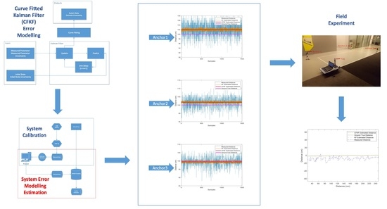
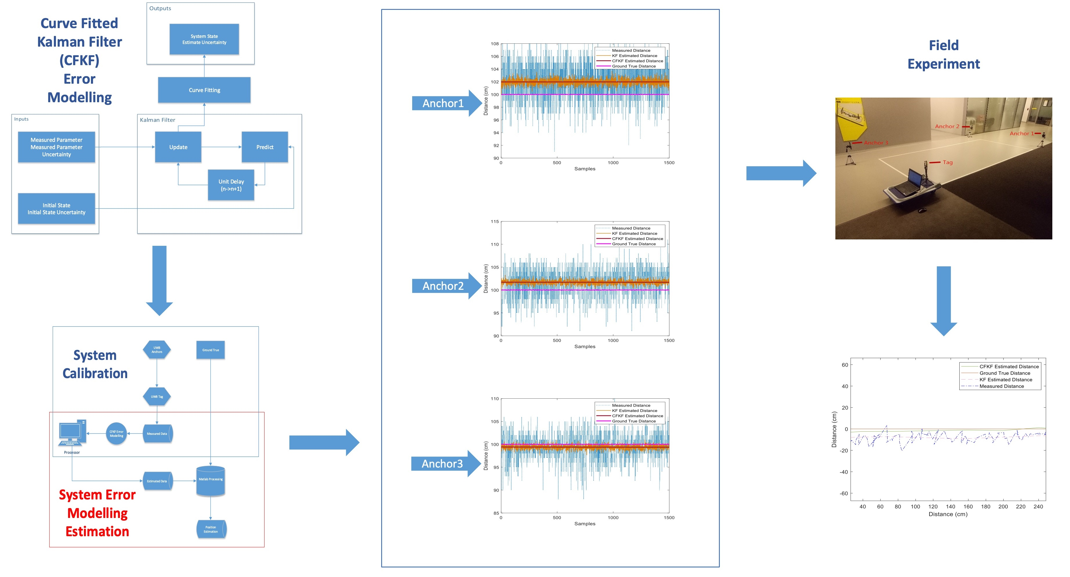
  • The calibration and experimental measurements from the ToF method in the UWB system using a curve fitting algorithm.
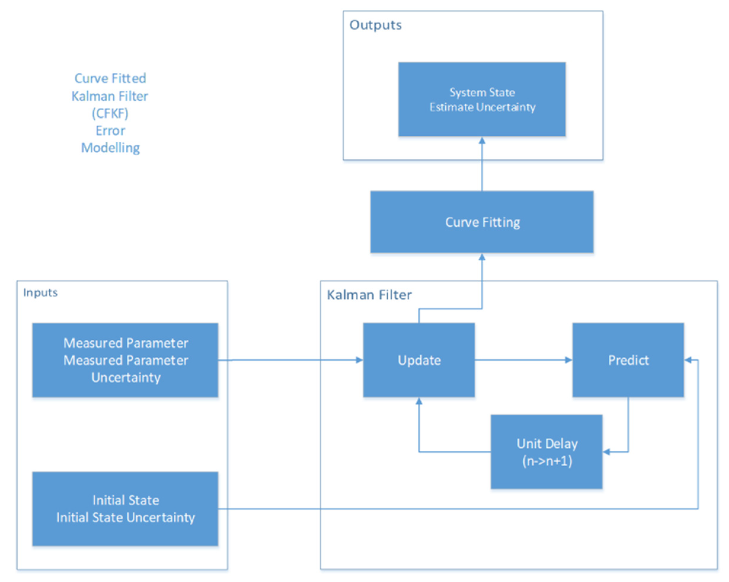
  • A novel CFKF error modelling has been developed to optimize the experiment’s estimation accuracy for UWB indoor localization systems.
  • A developed least squares algorithm (LSA)-based CFKF error modelling is proposed to improve the accuracy of the distance and coordinate for the UWB moving tag in the field experiment.
This paper is structured as follows: Section 2 introduces the proposed method of CFKF error modelling. In Section 3, UWB localization experiments are presented, including experiment calibration, error modelling processing and field experiment. In Section 4, the conclusions are discussed.

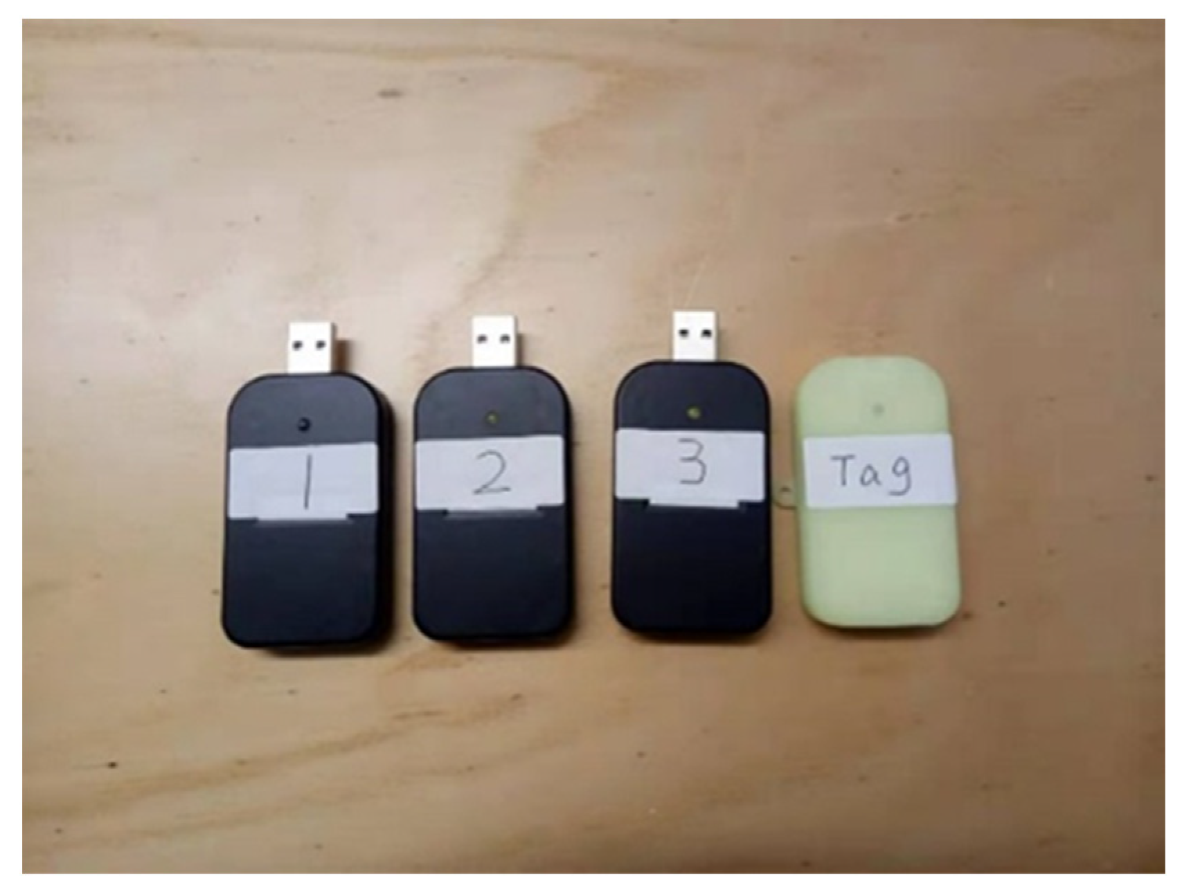
2. Materials and Methods

In this section, we propose a CFKF error modelling to optimize the localization accuracy. In general, KF has been implemented to estimate and update the system state by processing the measured data received from the UWB tag. However, most of the uncertainties are from data measurements, such as vibration noise, environment noise and system noise. To avoid those noises and improve the accuracy, data processed by KF are curve fitted by LSA. Figure 1. presents the workflow chart of CFKF error modelling.
The initial state update estimate equation of KF is
x ^ n , n = x ^ n , n 1 + K n ( z n x ^ n , n 1 H ) = ( 1 K n H ) x ^ n , n 1 + K n z n
The curve fitting algorithm is presented as follows:
y i = a 0 + a 1 x i + a 2 x i 2 + + a k x i k + ε i ( i = 1 , 2 , , n )
[ y 1 y 2 y 3 y n ] = [ 1 1 1 x 1 x 1 2 x 1 k x 2 x 2 2 x 2 k x 3 x 3 2 x 3 k 1             x n x n 2 x n k ]   [ a 1 a 2 a 3 a k ] + [ ε 1 ε 2 ε 3 ε n ]
To best match the LSA, we state that k = 1 and the curve fitting algorithm is initialized as the following:
y i = a x i + ε    
Here, we amend state update estimate equation of KF by using LSA.
y ^ n , n = a x ^ n , n + ε = a x ^ n , n 1 + a K n ( z n x ^ n , n 1 H ) + ε = a ( 1 K n H ) x ^ n , n 1 + a K n z n + ε
According to the derivation of LSA,
a = ( x ^ n , n 2 ) ( y ^ n , n ) ( x ^ n , n ) ( y ^ n , n ) n ( x ^ n , n 2 ) ( x ^ n , n ) 2
ε = n ( x ^ n , n y ^ n , n ) ( x ^ n , n ) ( y ^ n , n ) n ( x ^ n , n 2 ) ( x ^ n , n ) 2
Therefore,
y ^ n , n = ( x ^ n , n 2 ) ( y ^ n , n ) ( x ^ n , n ) ( y ^ n , n ) n ( x ^ n , n 2 ) ( x ^ n , n ) 2 x ^ n , n + n ( x ^ n , n y ^ n , n ) ( x ^ n , n ) ( y ^ n , n ) n ( x ^ n , n 2 ) ( x ^ n , n ) 2
The novel state update equation of KF is developed as follows:
y ^ n , n = ( x ^ n , n 2 ) ( y ^ n , n ) ( x ^ n , n ) ( y ^ n , n ) n ( x ^ n , n 2 ) ( x ^ n , n ) 2 ( 1 K n H ) x ^ n , n 1 + ( x ^ n , n 2 ) ( y ^ n , n ) ( x ^ n , n ) ( y ^ n , n ) n ( x ^ n , n 2 ) ( x ^ n , n ) 2 K n z n + n ( x ^ n , n y ^ n , n ) ( x ^ n , n ) ( y ^ n , n ) n ( x ^ n , n 2 ) ( x ^ n , n ) 2
The measured value is curve fitted to estimate the current state. The measurement uncertainty is also calculated by the curve fitting process to determine the Kalman gain ( K n ) from Equation (10).
K n = P n , n 1 H T H P n , n 1 H T + R n
The covariance update equation is
P n , n = ( I K n H ) P n , n 1 ( I K n H ) T + K n R n K n T
The predictor covariance equation is
P n + 1 , n = F P n , n F T + Q n
The predictor state equation is
x ^ n + 1 , n = F x ^ n , n + G u ^ n , n
F = [ 1 Δ t 0 1 ] ,   Δ t = 0.067 s ,   as   the   data   reflash   rate   is   15   Hz .
H = [ 10 ]
Q n = E ( ω n ω n T )
R n = E ( υ n υ n T )
where K n denotes the Kalman gain. P n , n 1 denotes the extrapolated estimate uncertainty. R n denotes the measurement uncertainty. x ^ 1 , 0 denotes the initial system state. P 1 , 0 denotes the initial state uncertainty. P n , n denotes the estimate uncertainty.     z n denotes the measured system state. x ^ n , n denotes the system state estimate. x ^ n , n 1 denotes the previous system state estimate. F denotes the state transition matrix. Q n denotes the process noise uncertainty. H denotes the observation matrix. u ^ n , n denotes the control vector. a denotes the scale factor error. ε denotes the bias error. ω n denotes the process noise. υ n denotes the measurement noise.
In Figure 2, the UWB anchors and tag used in the experiment are BooStar-T models, which are manufactured by Boocax. The specification of those UWB is presented in Table 1.

3. Results and Discussion

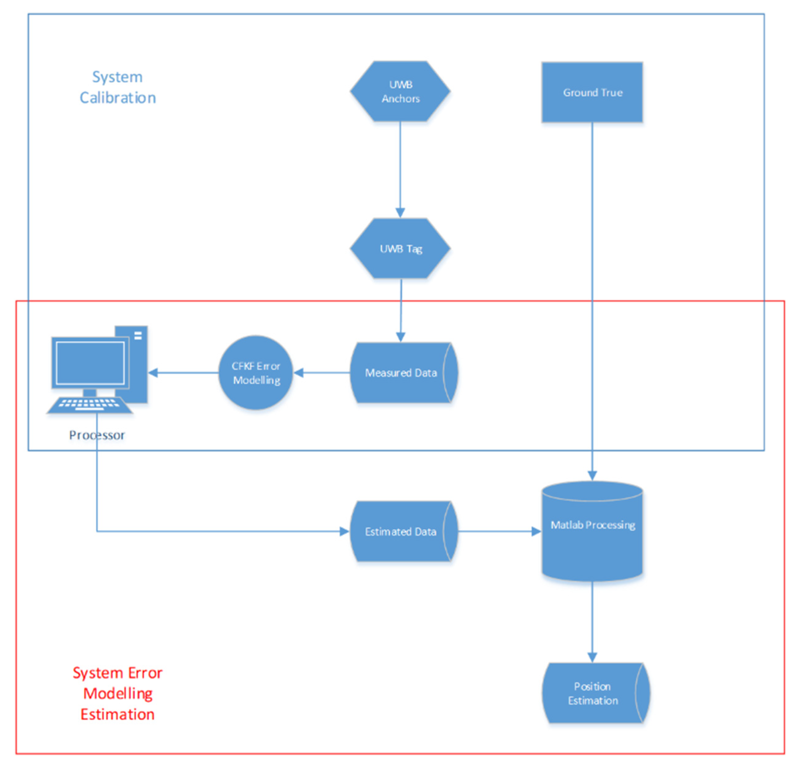
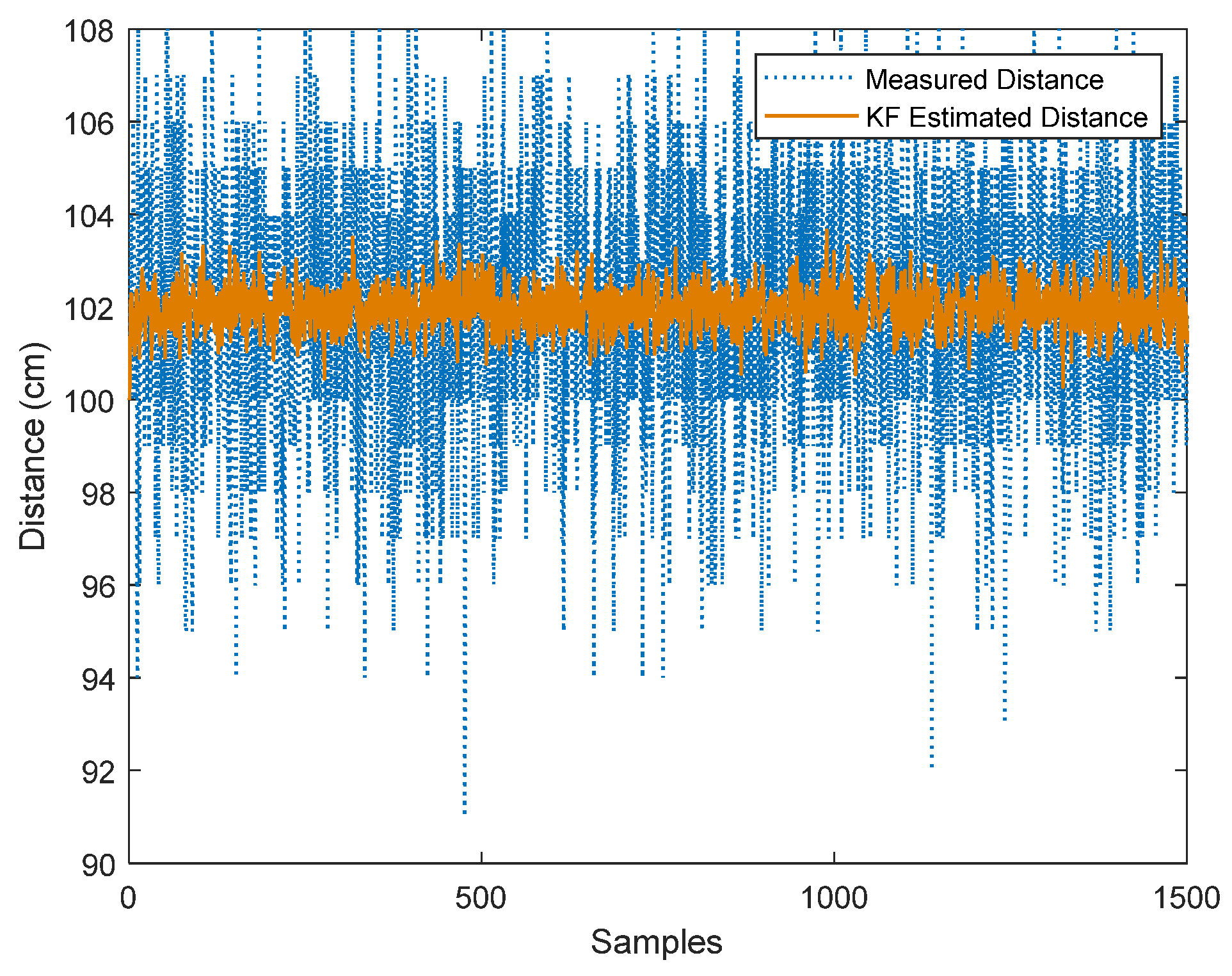
3.1. UWB Calibration Process for Distance

In the experiment, the CFKF error modelling is processed in the system calibration stage. The UWB anchor transmits the data to the UWB tag. According to the ToF method, the measured data of the distance have been calculated. The CFKF error modelling is implemented to minimize the uncertainties. The position data are updated from the calibration results. Figure 3 displays the workflow of the system.
The experiment testbed of the calibration process has been set up. Figure 4 displays the testbed set up from two different views.
In the testbed, the UWB tag is set up on a stand 50 cm high. The height of 50 cm is designed to avoid signal reflection from the ground. A USB data cable from the UWB tag is connected to the laptop to communicate with the UWB anchor synchronously and absorb the power from the laptop USB port. The UWB anchor is also set up on another stand with the same height one meter away from the UWB tag. A USB port power bank is connected to the UWB anchor to provide power.
As Figure 4 displays, both the tag and anchor are mounted on two 50 cm high stands with 1 meter distance in between. This testbed has been set up to calibrate the distance measurement for three different anchors named anchor 1, anchor 2 and anchor 3. The table below is a list of sample data for anchor 1, which are received by the UWB tag. The data contain Tag No., Time (ms), Anchor ID, and Distance (cm). In Table 2, some samples of the data can be found.

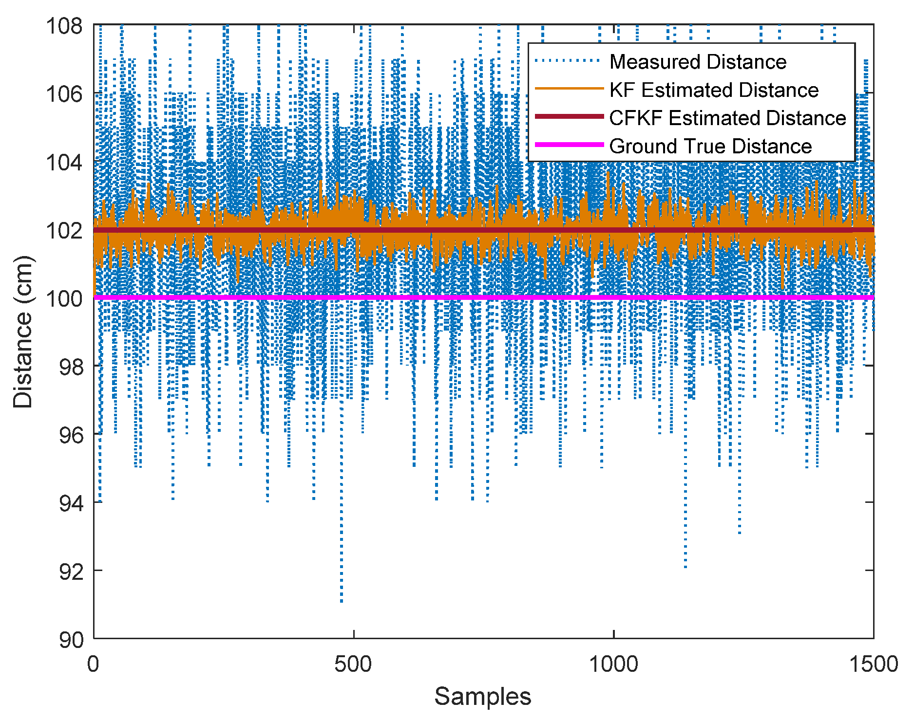
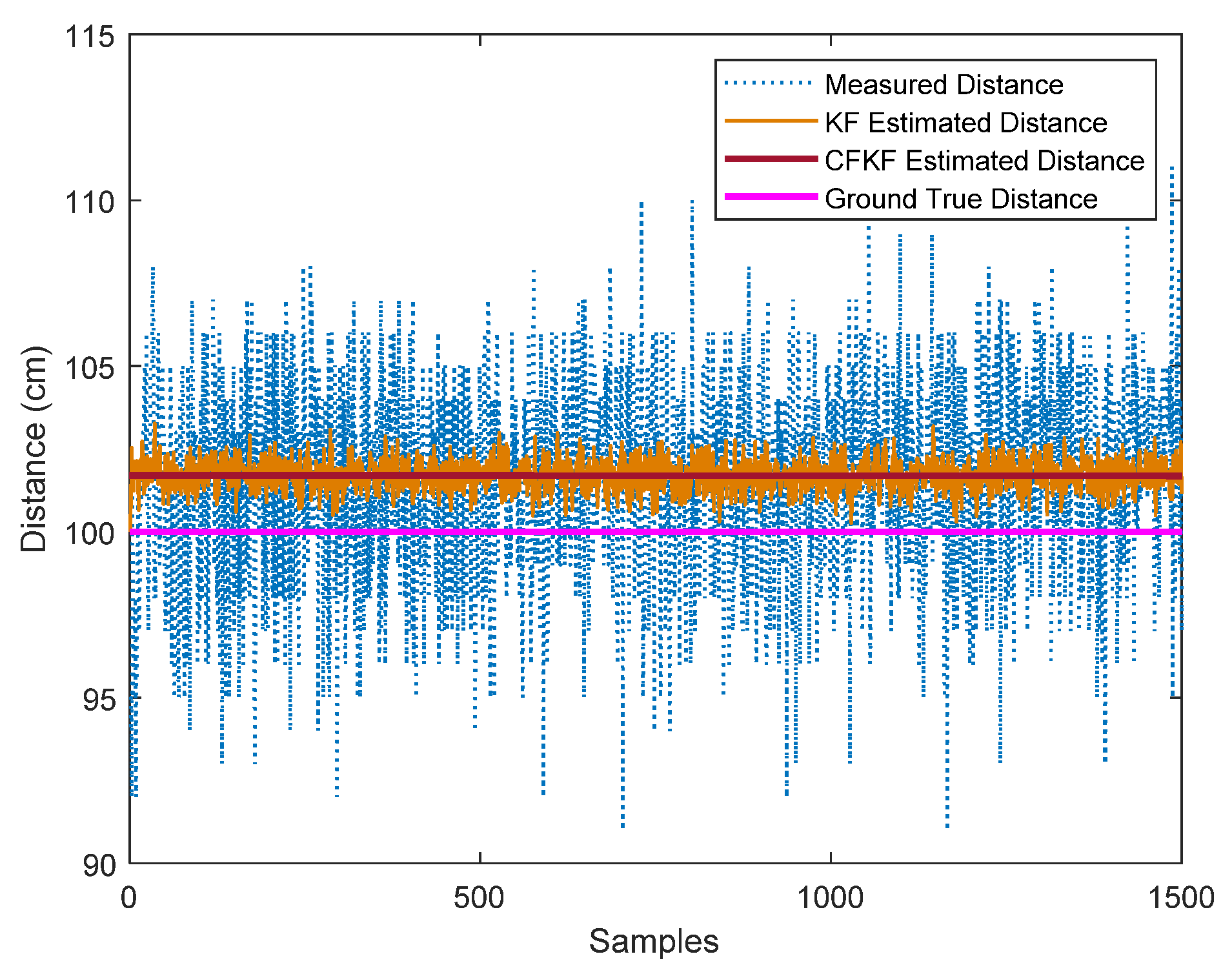
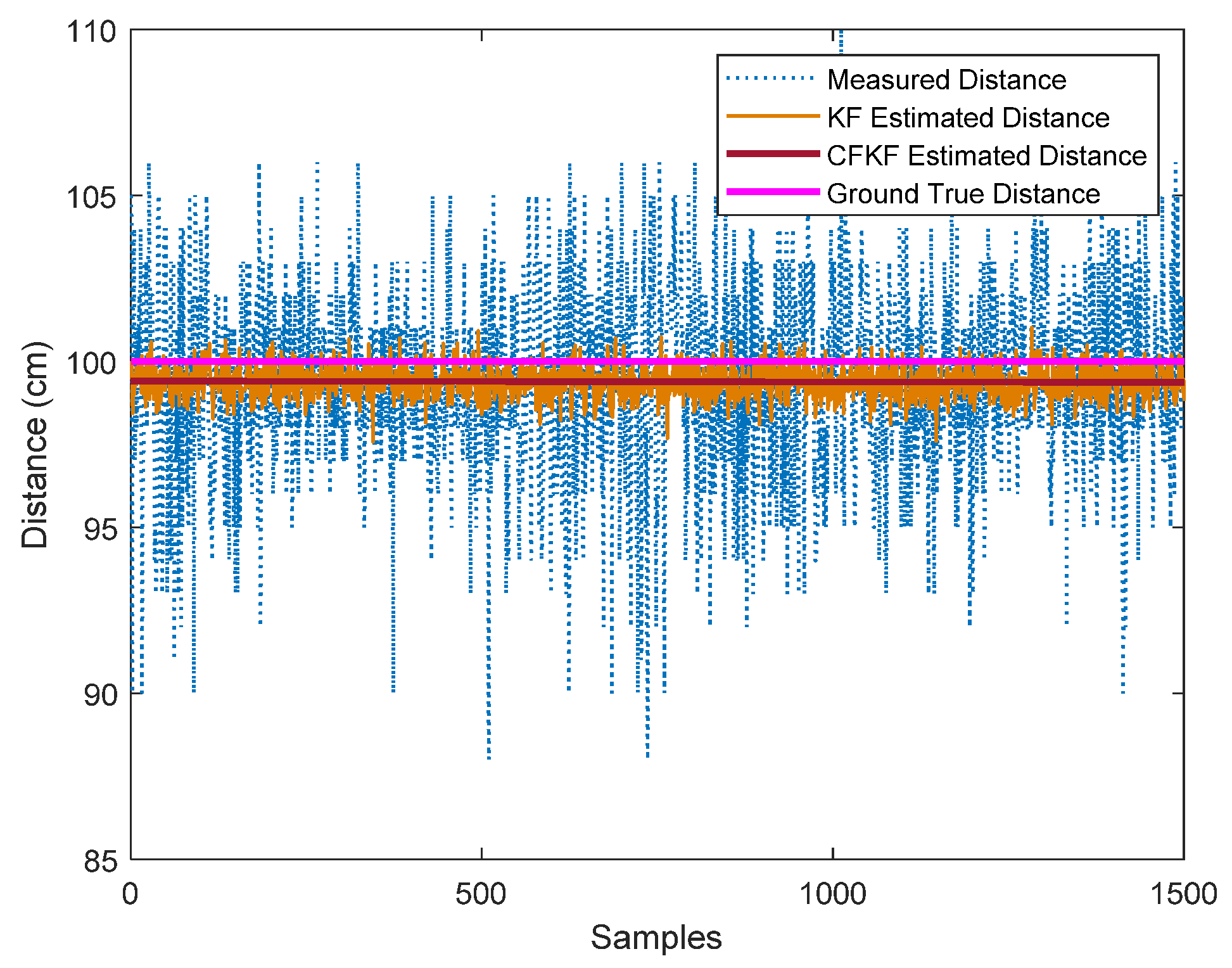
3.2. Error Modelling Calibration for UWB Anchors

Figure 5 displays the data sets of 1500 samples of the measured distance between UWB anchor 1 and tag. The blue lines represent the measured data of distance, whereas the red line represents the KF estimated data. When we use KF to process the measured data, the noises are reduced.
In Figure 6, when we use the curve fitting algorithm on the KF estimated data, the noises are further reduced and the result is more accurate than the estimated data from KF only.
For error modelling (CFKF),
y ^ n , n = a x ^ n , n + ε
For the coefficients (with 95% confidence bounds),
a   =   3.215 × 10 5   ( 2.178 × 10 5 ,   8.608 × 10 5 )
ε = 101.9 ( 101.9 , 102 )
The average value of a is 3.215 × 10⁻⁵. The range of a is from −2.178 × 10⁻⁵ (min) to 8.608 × 10⁻⁵ (max). The average value of ε is 101.9 and the range of ε is from 101.9 (min) to 102 (max). The ground true distance is 100 cm and the bias of CFKF estimated value is about 1.9 cm. Therefore, the coefficient a plays a small role, whereas the bias error ε accounts for much more. These could be manufactory errors, as each anchor contains different values of a and ε . To reduce the main error from the anchors, bias error ε should be minimized.

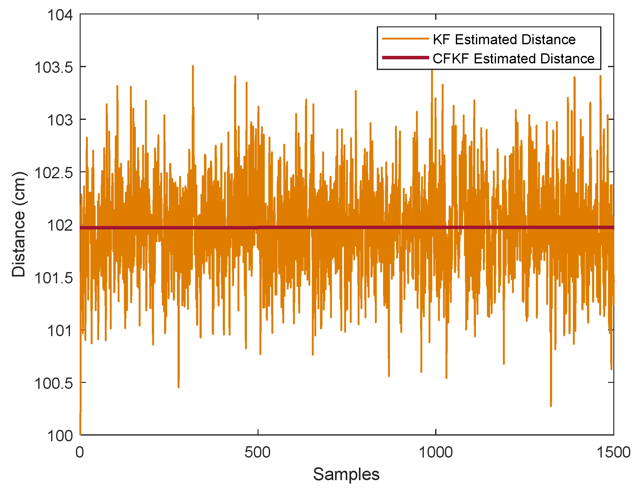
3.3. Error Modelling Optimized Calibration Results

To distinguish between the optimized calibration results for UWB anchor 1 from the error modelling, we merge Figure 5 and Figure 6 into Figure 7 and add the ground true distance. As Figure 7 illustrates, the blue line presents the measured distance, the pink line displays the ground true, the orange line presents the KF estimated distance and the brown line represents the CFKF estimated distance. We can clearly determine that the CFKF estimated results are the most accurate, as they are the closest results to the ground true distance compared to the other methods. In the same testbed, the calibration process is repeated by using different anchors. Figure 8 and Figure 9 present the calibration results for anchor 2 and anchor 3. The error results are recorded in Table 3; we can observe that the error rate from CFKF is much lower than the methods for all three anchors. During the calibration, the CFKF error modelling has optimized the result of the estimated positioning data. At the next stage, the actual study of moving objects in a dynamic environment has been set up and processed.
Several different algorithms have been used to determine the best method for calibration at this stage. We gather all the results for anchor 1 into the same plot. As Figure 7 presents, the CFKF estimated distance is closer to the ground true distance than the other methods. In the same testbed, the calibration process is repeated by using different anchors. Figure 8 and Figure 9 present the calibration result for anchor 2 and anchor 3. The bias uncertainty results are recorded in Table 3; we can observe that the bias uncertainty rate from CFKF is much lower than the methods for all three anchors. During the calibration, the CFKF error modelling has determined the bias uncertainties for each anchor. By minimizing these bias uncertainties, we can optimize the result accuracy of the estimated positioning data. At the next stage, the actual study of moving objects in a dynamic environment has been set up and processed.

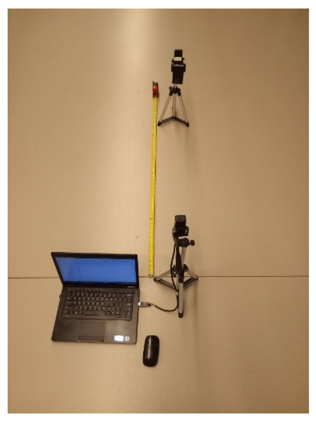
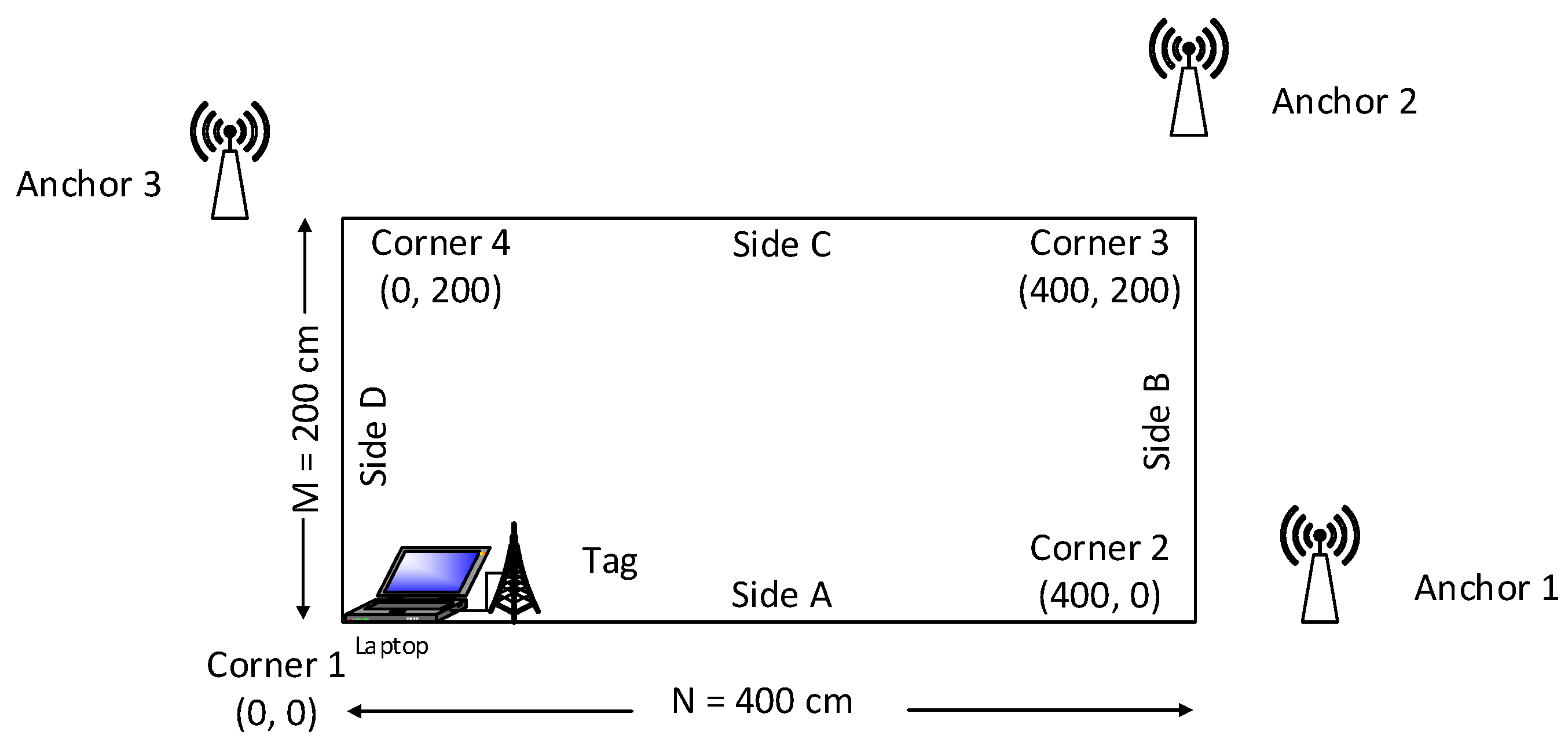
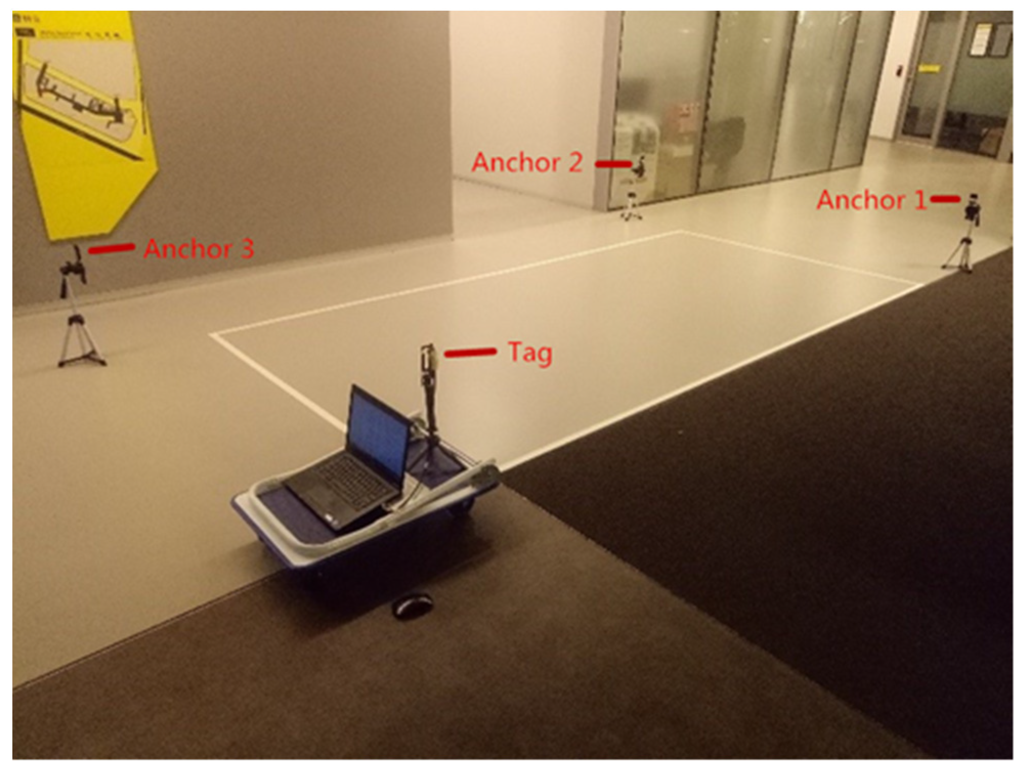
3.4. Field Experiment of UWB Localization

In this field experiment of UWB localization, the testbed is set up for a real-time moving platform. This field experiment aims to validate the accuracy of the CFKF error modelling in a dynamic scenario.
Figure 10 displays the floor plan for the testbed. Corner 1 has been set up as the coordinate origin (0, 0), where N = 0 and M = 0. Side A is set up on the x axis and side D is set up on the y axis. Therefore, the coordinate of corner 2 should be (400, 0), where N = 400 cm and M = 0. The coordinate of corner 3 should be (400, 200), where N = 400 cm and M = 200 cm. The coordinate of corner 4 should be (0, 200), where N = 0 cm and M = 200 cm.
The testbed has been set up, as Figure 11 displays. There is a white rectangle on the ground. The length and width of the rectangle are 400 cm and 200 cm. Anchor 1 has been mounted on the stand that is 50 cm high. It is set up in the same line as side A, but is 50 cm away from corner 2. In the same way as Anchor 2 and Anchor 3, they have been mounted on the stand that is 50 cm high. They are set up in the same line as side B and side C, but are 50 cm away from corner 3 and corner 4. The anchors are set up 50 cm away from the rectangle to avoid the moving platform touching the anchors when it moves to the corner. The tag mounted on the stand has been set up on the moving platform with the same height, 50 cm in total, including the platform height. A laptop is connected to the tag to log the real-time data.
In this field experiment, a UWB tag is set up on a designed moving platform with a laptop connected for logging data synchronously. The moving platform starts to move from corner 1. When it arrives at the rectangle corner 2, it turns 90° left to continue to move along side B to corner 3. The platform keeps moving until it arrives at the original start point corner 1. During the period, anchor 1, anchor 2 and anchor 3 keep sending data to the tag. The UWB tag on the platform receives the data from all anchors and logs the data into the laptop synchronously. The trilateration method is used for the three anchors and one tag UWB localization system to calculate the distance and coordinate of the moving object.
Firstly, from the Pythagorean theorem,
{ ( N 1 N ) 2 + ( M 1 M ) 2 = d 1 2 ( N n N ) 2 + ( M n M ) 2 = d n 2
Secondly, when using the ( n 1 ) t h function minus the n t h function to generate the linear Equation (22), n is the anchors’ number.
A X = b
when
A = [ 2 ( N 1 N 3 ) 2 ( M 1 M 3 ) 2 ( N 2 N 3 ) 2 ( M 2 M 3 ) ]
b = [ N 1 2 N 3 2 + M 1 2 M 3 2 + d 3 2 d 1 2 N 2 2 N 3 2 + M 2 2 M 3 2 + d 3 2 d 2 2 ]
After using LSA,
X = ( A T A ) 1 A T b
X = [ N M ]
X ( N , M ) is the coordinate of the moving tag from the device measurement.

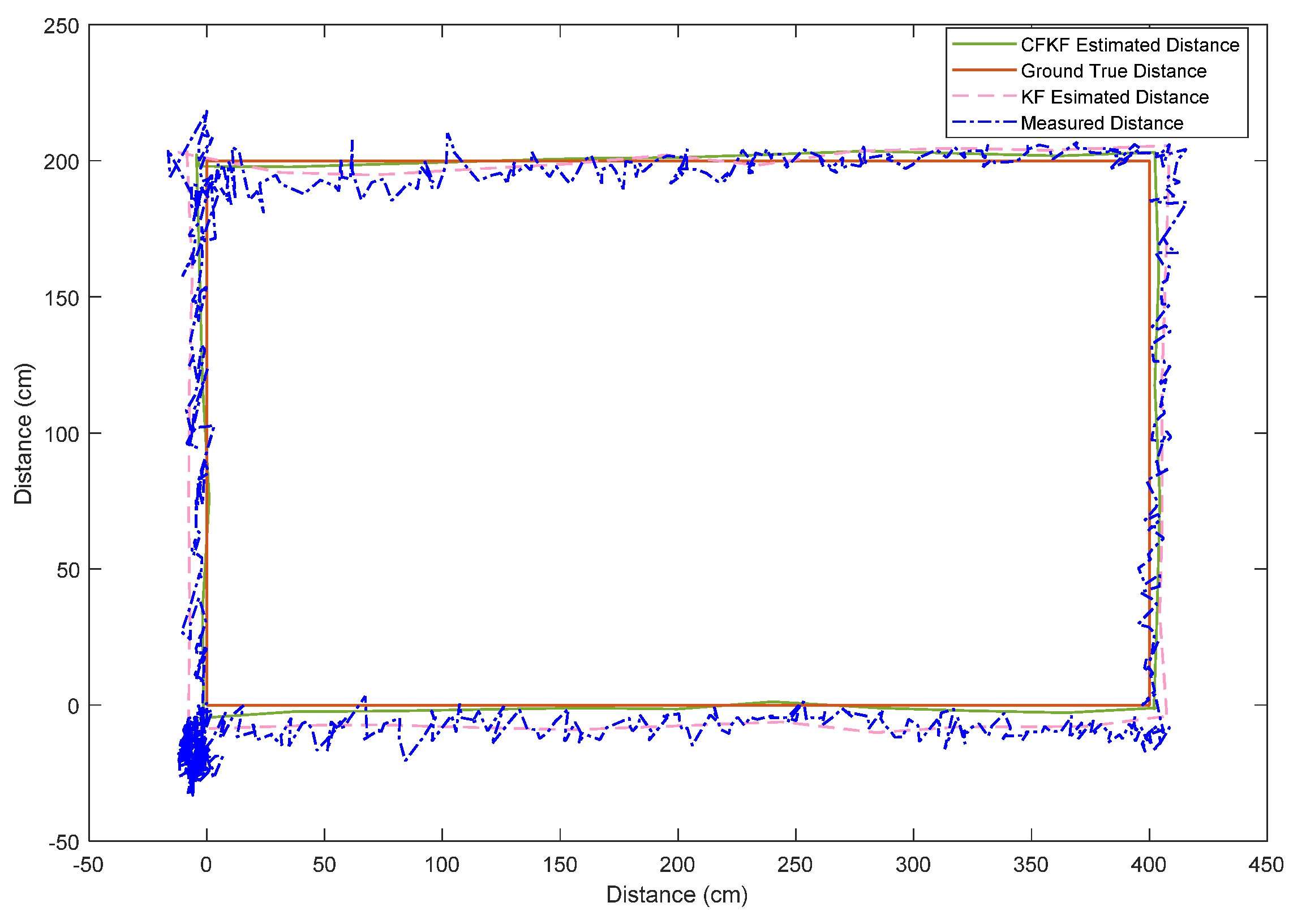
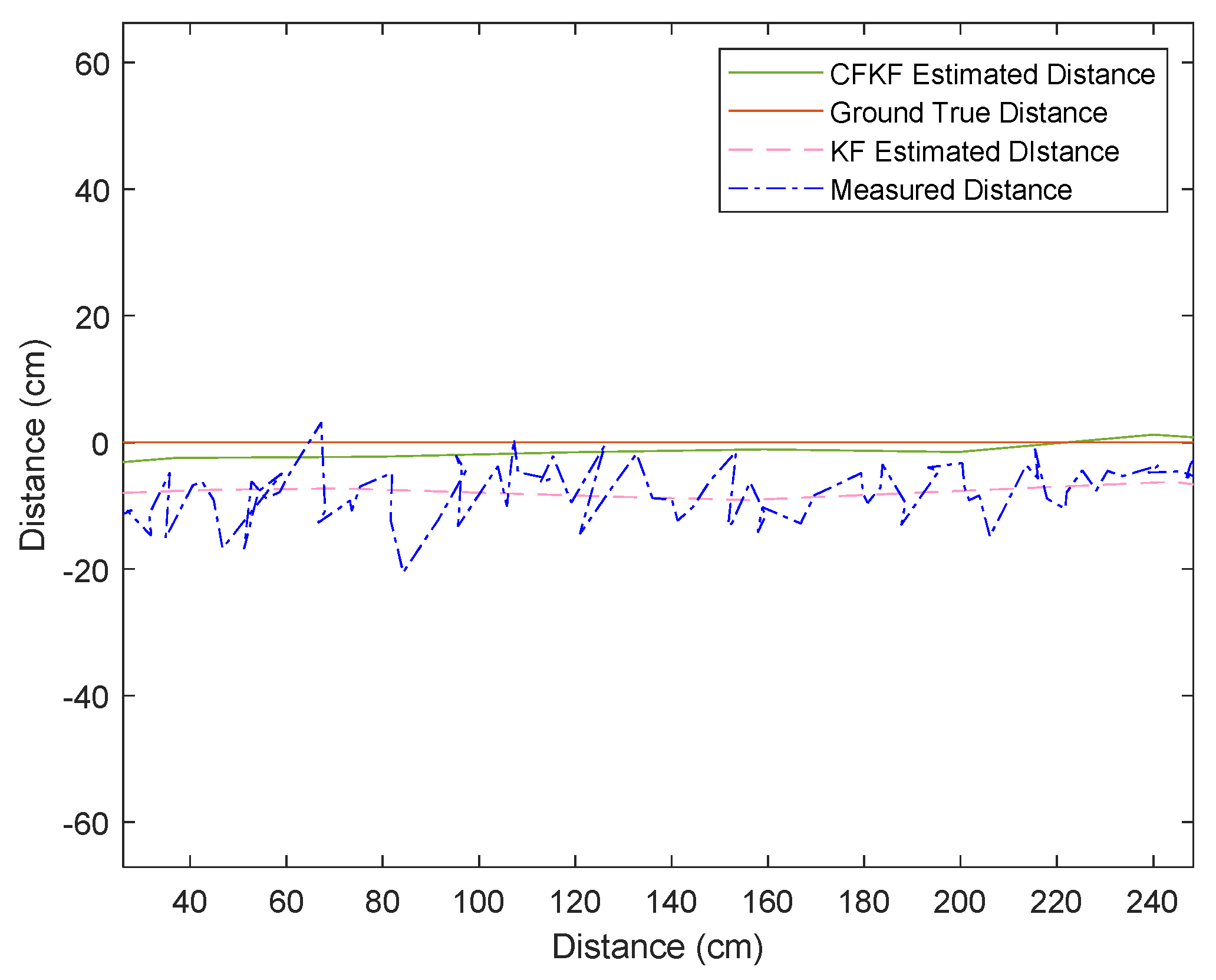
3.5. Experiment Results and Discussion

As Figure 12 illustrates, the blue dotted line is the measured distance from the UWB tag. The manufactory error of the UWB system is about 20 cm. At corner 1, there is a large blue area near the coordinate origin; this is when the platform gets ready for a few seconds and starts to move. Due to the manufactory error, the measured distance is about 2–20 cm away from the coordinate (0, 0). The pink dotted line is the data for the KF estimated distance, as shown in Figure 12. The pink line reduced the noise; it is smoother than the blue line. However, compared with the red line (ground true distance), it still contains uncertainties from the ground true data. Figure 13 is the zoomed plot of the part of Figure 12. It indicates that the KF estimated distance, the pink line, contains about 2–10 cm uncertainties from the ground true distance, whereas the CFKF estimated distance, the green line, contains 1–2 cm uncertainties. Figure 12 and Figure 13 clearly show that the green line is much closer to the ground true red line than the others. Using Table 4, we can calculate that the accuracy has been improved by about 1–8%. Compared with the raw measured distance, the accuracy has been optimized by about 1–18%.
In this section, the UWB localization system has been investigated. Three anchors and one tag have been set up in the testbed. The different anchor may have different manufactory errors. An individual calibration process has been applied. The field experiment can be described as dynamic research and a developed LSA-based CFKF error modelling is used to determine the distance and coordinate of the moving object. According to the results displayed in Table 3, when the experiment uses anchor 1, the uncertainty rate from the measurement results is 4.5%, the uncertainty rate from the KF results is 2.4%, and the error rate from the CFKF error modelling algorithm results is 1.9%. The uncertainty rate from the KF results is higher than the CFKF error modelling algorithm results. Therefore, the CFKF error modelling algorithm results are about 2.6% more accurate than the results from the measurement, and are 0.5% more accurate than the results from the KF. For anchor 2, the uncertainty rates are as follows: measurement (3.7%), KF (2.1%) and CFKF error modelling algorithm (1.7%). For anchor 3, the uncertainty rates are as follows: measurement (3.2%), KF (1.5%) and CFKF error modelling algorithm (0.6%). For the field experiment, the uncertainty rates are recorded in Table 4 and are as follows: measurement (2–20%), KF (2–10%) and CFKF error modelling algorithm (1–2%). According to all the records, it is validated that the results from the CFKF error modelling algorithm are the most accurate and that this is the most robust method for the UWB system.

4. Conclusions

This article presents a novel contribution to the UWB localization field by the proposed novel CFKF error modelling algorithm. The novel error modelling algorithm has been implemented in both the calibration process and field experiment. In the UWB systems, three UWB anchors and one UWB tag have been implemented in the research. The CFKF error modelling optimized the calibration results. It is more accurate than the other methods used. The field experiment is a dynamic validation of the error modelling. The results validate that the CFKF error modelling produces a significant improvement in the accuracy of the system. In this article, we have validated most experiments in the linear environment. In future research, we will focus on the non-linear environment. Error modeling, such as the curve fitted extended Kalman filter (CFEKF) and curve fitted unscented Kalman filter, (CFUKF) will be continuously developed in our research on non-linear situations. Moreover, more localization sensors will be added into the system and all the data could be fused in the same system and optimized by the same error modelling. Further implementation of sensors will be developed, including radar, ultrasonic, and infrared systems. All the algorithms can be switched to calculate different data from different environments to improve the accuracy of error modelling.

Author Contributions

Conceptualization, Z.Y.; Data curation, Z.Y. and J.S.; Formal analysis, Z.Y. and J.S.; Investigation, Z.Y.; Methodology, Z.Y. and J.S.; Project administration, Z.C.; Resources, Z.C.; Software, Z.Y.; Supervision, Z.C.; Validation, J.S.; Visualization, Z.Y.; Writing—original draft, Z.Y.; Writing—review & editing, J.S. All authors have read and agreed to the published version of the manuscript.

Funding

The authors gratefully acknowledge the financial support from the National Natural Science Foundation of China (Grant No. 12102203, 61901235), the Natural Science Foundation of Jiangsu Province (Grant No. BK20200971).

Data Availability Statement

Not applicable.

Conflicts of Interest

The authors declare no conflict of interest.

References

  1. Li, Y.-Y.; Qi, G.-Q.; Sheng, A.-D. Performance Metric on the Best Achievable Accuracy for Hybrid TOA/AOA Target Localization. IEEE Commun. Lett. 2018, 22, 1474–1477. [Google Scholar] [CrossRef]
  2. Mimoune, K.-M.; Ahriz, I.; Guillory, J. Evaluation and Improvement of Localization Algorithms Based on UWB Pozyx System. In Proceedings of the 2019 International Conference on Software, Telecommunications and Computer Networks (SoftCOM), Split, Croatia, 19–21 September 2019. [Google Scholar] [CrossRef]
  3. Ni, D.; Postolache, O.A.; Mi, C.; Zhong, M.; Wang, Y. UWB Indoor Positioning Application Based on Kalman Filter and 3-D TOA Localization Algorithm. In Proceedings of the 2019 11th International Symposium on Advanced Topics in Electrical Engineering (ATEE), Bucharest, Romania, 28–30 March 2019; pp. 1–6. [Google Scholar] [CrossRef]
  4. Peng, W.; Zhao, X.; Jiang, T.; Adachi, F. PRIDE: Path Integration Based Delay Estimation in Multi-Device Multi-Path Environments. IEEE Trans. Veh. Technol. 2018, 67, 11587–11596. [Google Scholar] [CrossRef]
  5. Piccinni, G.; Torelli, F.; Avitabile, G. Distance Estimation Algorithm for Wireless Localization Systems Based on Lyapunov Sensitivity Theory. IEEE Access 2019, 7, 158338–158348. [Google Scholar] [CrossRef]
  6. Wang, M.; Xue, B.; Wang, W.; Yang, J. The design of multi-user indoor UWB localization system. In Proceedings of the 2017 2nd International Conference on Frontiers of Sensors Technologies (ICFST), Shenzhen, China, 14–16 April 2017; pp. 322–326. [Google Scholar] [CrossRef]
  7. Shang, F.; Champagne, B.; Psaromiligkos, I.N. A ML-Based Framework for Joint TOA/AOA Estimation of UWB Pulses in Dense Multipath Environments. IEEE Trans. Wirel. Commun. 2014, 13, 5305–5318. [Google Scholar] [CrossRef]
  8. Bulten, W. Kalman Filters Explained: Removing Noise from RSSI Signals. 2015. Available online: https://www.wouterbulten.nl/blog/tech/kalman-filtersexplained-removing-noise-from-rssi-signals (accessed on 11 August 2022).
  9. Ding, G.; Zhang, J.; Zhang, L.; Tan, Z. Overview of received signal strength based fingerprinting localization in indoor wireless LAN environments. In Proceedings of the 2013 5th IEEE International Symposium on Microwave, Antenna, Propagation and EMC Technologies for Wireless Communications, Chengdu, China, 29–31 October 2013; pp. 160–164. [Google Scholar] [CrossRef]
  10. Iglesias, H.J.P.; Barral, V.; Escudero, C.J. Indoor person localization system through RSSI Bluetooth fingerprinting. In Proceedings of the 2012 19th International Conference on Systems, Signals and Image Processing (IWSSIP), Vienna, Austria, 11–13 April 2012; pp. 40–43. [Google Scholar]
  11. Papamanthou, C.; Preparata, F.P.; Tamassia, R. Algorithms for location estimation based on RSSI sampling. In International Symposium on Algorithms and Experiments for Sensor Systems, Wireless Networks and Distributed Robotics; Springer: Berlin/Heidelberg, Germany, 2008; pp. 72–86. [Google Scholar]
  12. Wang, J.-Y.; Chen, C.-P.; Lin, T.-S.; Chuang, C.-L.; Lai, T.-Y.; Jiang, J.-A. High-Precision RSSI-based Indoor Localization Using a Transmission Power Adjustment Strategy for Wireless Sensor Networks. In Proceedings of the 2012 IEEE 14th International Conference on High Performance Computing and Communication & 2012 IEEE 9th International Conference on Embedded Software and Systems, Liverpool, UK, 25–27 June 2012; pp. 1634–1638. [Google Scholar] [CrossRef]
  13. Huang, S.; Chen, J.; Jiang, H. UWB indoor location based on improved least square support vector machine considering anchor anomaly. In Proceedings of the 2020 IEEE 16th International Conference on Control & Automation (ICCA), Singapore, 9–11 October 2020; pp. 324–329. [Google Scholar] [CrossRef]
  14. Piccinni, G.; Avitabile, G.; Coviello, G.; Talarico, C. Real-Time Distance Evaluation System for Wireless Localization. IEEE Trans. Circuits Syst. I Regul. Pap. 2020, 67, 3320–3330. [Google Scholar] [CrossRef]
  15. Cui, X.; Li, J.; Wu, C.; Liu, J.-H. A Timing Estimation Method Based-on Skewness Analysis in Vehicular Wireless Networks. Sensors 2015, 15, 28942–28959. [Google Scholar] [CrossRef]
  16. Liang, X.; Zhang, H.; Gulliver, T.A. Energy Detector based Time of Arrival Estimation using a Neural Network with Millimeter Wave Signals. KSII Trans. Internet Inf. Syst. 2016, 10, 3050–3065. [Google Scholar]
  17. Liang, X.; Zhang, H.; Lu, T.; Gulliver, T.A. Energy detector based TOA estimation for MMW systems using machine learning. Telecommun. Syst. 2017, 64, 417–427. [Google Scholar] [CrossRef]
  18. Guvenc, I.; Şahinoğlu, Z. Threshold selection for UWB TOA estimation based on kurtosis analysis. IEEE Commun. Lett. 2005, 9, 1025–1027. [Google Scholar] [CrossRef]
  19. Ding, R.; Qian, Z.-H.; Wang, X. UWB Positioning System Based on Joint TOA and DOA Estimation. J. Electron. Inf. Technol. 2010, 32, 313–317. [Google Scholar] [CrossRef]
  20. Li, X.; Cao, F. Location Based TOA Algorithm for UWB Wireless Body Area Networks. In Proceedings of the 2014 IEEE 12th International Conference on Dependable, Autonomic and Secure Computing, Dalian, China, 24–27 August 2014; pp. 507–511. [Google Scholar] [CrossRef]
  21. Wang, T.; Chen, X.; Ge, N.; Pei, Y. Error analysis and experimental study on indoor UWB TDoA localization with reference tag. In Proceedings of the 2013 19th Asia-Pacific Conference on Communications (APCC), Denpasar, Bali Island, 29–31 August 2013; pp. 505–508. [Google Scholar] [CrossRef]
  22. Adams, J.C.; Gregorwich, W.; Capots, L.; Liccardo, D. Ultra-wideband for navigation and communications. In Proceedings of the 2001 IEEE Aerospace Conference Proceedings (Cat. No. 01TH8542), Big Sky, MT, USA, 10–17 March 2001; Volume 2, pp. 785–792. [Google Scholar]
  23. Beuchat, P.N.; Hesse, H.; Domahidi, A.; Lygeros, J. Enabling Optimization-Based Localization for IoT Devices. IEEE Internet Things J. 2019, 6, 5639–5650. [Google Scholar] [CrossRef]
  24. Zhang, S.; Han, R.; Huang, W.; Wang, S.; Hao, Q. Linear Bayesian Filter Based Low-Cost UWB Systems for Indoor Mobile Robot Localization. In Proceedings of the 2018 IEEE SENSORS, New Delhi, India, 28–31 October 2018; pp. 1–4. [Google Scholar] [CrossRef]
  25. Alarifi, A.; Al-Salman, A.; Alsaleh, M.; Alnafessah, A.; Al-Hadhrami, S.; Al-Ammar, M.A.; Al-Khalifa, H.S. Ultra Wideband Indoor Positioning Technologies: Analysis and Recent Advances. Sensors 2016, 16, 707. [Google Scholar] [CrossRef] [PubMed] [Green Version]
  26. Yang, S.; Wang, B. Residual based weighted least square algorithm for bluetooth/UWB indoor localization system. In Proceedings of the 2017 36th Chinese Control Conference (CCC), Dalian, China, 26–28 July 2017; pp. 5959–5963. [Google Scholar] [CrossRef]
  27. Güvenç, I.; Chong, C.-C.; Watanabe, F.; Inamura, H. NLOS Identification and Weighted Least-Squares Localization for UWB Systems Using Multipath Channel Statistics. EURASIP J. Adv. Signal Process. 2007, 2008, 271984. [Google Scholar] [CrossRef]
  28. Dardari, D.; Conti, A.; Lien, J.; Win, M.Z. The effect of cooperation on localization systems using UWB experimental data. EURASIP J. Appl. Signal Process. 2008, 2008, 513873. [Google Scholar] [CrossRef]
  29. Molisch, A.F. Ultrawideband propagation channels-theory, measurement, and modeling. IEEE Trans. Veh. Technol. 2005, 54, 1528–1545. [Google Scholar] [CrossRef]
  30. Karedal, J.; Wyne, S.; Almers, P.; Tufvesson, F.; Molisch, A.F. A Measurement-Based Statistical Model for Industrial Ultra-Wideband Channels. IEEE Trans. Wirel. Commun. 2007, 6, 3028–3037. [Google Scholar] [CrossRef]
  31. Wymeersch, H.; Marano, S.; Gifford, W.M.; Win, M.Z. A Machine Learning Approach to Ranging Error Mitigation for UWB Localization. IEEE Trans. Commun. 2012, 60, 1719–1728. [Google Scholar] [CrossRef]
  32. Dong, F.; Shen, C.; Zhang, J.; Zhou, S. A TOF and Kalman filtering joint algorithm for IEEE802. 15.4 a UWB locating. In Proceedings of the 2016 IEEE Information Technology, Networking, Electronic and Automation Control Conference, Chongqing, China, 20–22 May 2016; pp. 948–951. [Google Scholar]
  33. Zhu, D.; Yi, K. EKF localization based on TDOA/RSS in underground mines using UWB ranging. In Proceedings of the 2011 IEEE International Conference on Signal Processing, Communications and Computing (ICSPCC), Xi’an, China, 14–16 September 2011; pp. 1–4. [Google Scholar] [CrossRef]
  34. Yan, L.; Lu, Y.; Zhang, Y. An Improved NLOS Identification and Mitigation Approach for Target Tracking in Wireless Sensor Networks. IEEE Access 2017, 5, 2798–2807. [Google Scholar] [CrossRef]
  35. Lategahn, J.; Muller, M.; Rohrig, C. TDoA and RSS Based Extended Kalman Filter for Indoor Person Localization. In Proceedings of the 2013 IEEE 78th Vehicular Technology Conference (VTC Fall), Las Vegas, NV, USA, 2–5 September 2013; pp. 1–5. [Google Scholar] [CrossRef]
Figure 1. Workflow chart of CFKF error modelling.
Remotesensing 14 04902 g001
Figure 2. Three UWB Anchors and one UWB tag.
Remotesensing 14 04902 g002
Figure 3. System calibration and error modelling estimation for UWB localization.
Remotesensing 14 04902 g003
Figure 4. Testbed setup for 1-m distance range for UWB localization.
Remotesensing 14 04902 g004
Figure 5. Comparison of the measured distance and KF estimated distance (UWB anchor 1).
Remotesensing 14 04902 g005
Figure 6. Comparison of the KF estimated distance and CFKF estimated distance (UWB anchor 1).
Remotesensing 14 04902 g006
Figure 7. Error modelling calibration result comparison with different algorithms (UWB anchor 1).
Remotesensing 14 04902 g007
Figure 8. Error modelling calibration result comparison with different algorithms (UWB anchor 2).
Remotesensing 14 04902 g008
Figure 9. Error modelling calibration result comparison with different algorithms (UWB anchor 3).
Remotesensing 14 04902 g009
Figure 10. Floor plan for the testbed of UWB field experiment.
Remotesensing 14 04902 g010
Figure 11. Testbed for UWB field experiment.
Remotesensing 14 04902 g011
Figure 12. Comparison of different algorithm results in the UWB field experiment.
Remotesensing 14 04902 g012
Figure 13. Zoomed comparison of different algorithm results in the UWB field experiment.
Remotesensing 14 04902 g013
Table 1. UWB anchor and tag specification.
NameSpecification
Measurement MethodToF
Factory ErrorLine of Sight < 15 cm,
No Line of Sight < 30 cm
Positioning Accuracy<20 cm
Anchor Setup Range<100 m (Line of Sight)
Transmission Range<130 m (Line of Sight)
Tag NumberMax 7 in the System
Data Refresh RateSingle Tag 15 Hz
PowerAverage 0.5 W
Operating Temperature−40 °C to 85 °C
Operating Frequency6.2 GHz to 6.7 GHz
SizeAnchor: 82.5 mm × 38 mm × 11.5 mm,
Tag: 69 mm × 38 mm × 11.9 mm
Power SupplyDC 5V, 1A
Table 2. Sample data table for anchor 1.
Tag No.Time (ms)Anchor IDDistance (cm)
Tag No.: 126,151Anchor 1100
Tag No.: 126,207Anchor 1103
Tag No.: 126,263Anchor 1104
Tag No.: 126,319Anchor 1100
Tag No.: 126,375Anchor 1100
Tag No.: 126,431Anchor 1106
Tag No.: 126,488Anchor 1105
Tag No.: 126,544Anchor 1101
Tag No.: 126,600Anchor 1100
Tag No.: 126,688Anchor 1102
Tag No.: 126,744Anchor 1100
Tag No.: 126,800Anchor 194
Tag No.: 126,857Anchor 1108
Tag No.: 126,913Anchor 1102
Tag No.: 126,969Anchor 196
Tag No.: 127,025Anchor 1102
Tag No.: 127,081Anchor 1105
Tag No.: 127,137Anchor 1103
Tag No.: 127,225Anchor 1104
Tag No.: 127,282Anchor 1105
Tag No.: 127,338Anchor 1102
Table 3. Algorithm bias table for UWB anchor 1–3.
Positioning AlgorithmBias
(Centimeter)
Uncertainty Rate
Anchor 1
CFKF1.91.9%
KF2.42.4%
Measurement4.54.5%
Anchor 2
CFKF1.71.7%
KF2.12.1%
Measurement3.73.7%
Anchor 3
CFKF−0.60.6%
KF−1.51.5%
Measurement−3.23.2%
Table 4. Algorithm bias table for field experiment.
Positioning AlgorithmBias
(Centimeter)
Uncertainty Rate
CFKF1–21–2%
KF2–102–10%
Measurement 2–202–20%
Publisher’s Note: MDPI stays neutral with regard to jurisdictional claims in published maps and institutional affiliations.

