Improving the Modeling of Sea Surface Currents in the Persian Gulf and the Oman Sea Using Data Assimilation of Satellite Altimetry and Hydrographic Observations

Abstract

Sea surface currents are often modeled using numerical models without adequately addressing the issue of model calibration at the regional scale. The aim of this study is to calibrate the MIKE 21 numerical ocean model for the Persian Gulf and the Oman Sea to improve the sea surface currents obtained from the model. The calibration was performed through data assimilation of the model with altimetry and hydrographic observations using variational data assimilation, where the weights of the objective functions were defined based on the type of observations and optimized using metaheuristic optimization methods. According to the results, the calibration of the model generally led the model results closer to the observations. This was reflected in an improvement of about 0.09 m/s in the obtained sea surface currents. It also allowed for more accurate evaluations of model parameters, such as Smagorinsky and Manning coefficients. Moreover, the root mean square error values between the satellite altimetry observations at control stations and the assimilated model varied between 0.058 and 0.085 m. We further showed that the kinetic energy produced by sea surface currents could be used for generating electricity in the Oman Sea and near Jask harbor.

1. Introduction

For many years, geoscientists have been interested in the study of sea surface currents (SSCs) and their causes. As countries exchanged goods, food, etc. through the sea, the need to gain knowledge of ocean currents was felt, and they realized that, by understanding the process of SSCs, they could carry out economic activities more efficiently. The significance of modeling SSCs in different water bodies, such as rivers, lakes, and open seas, is crucial for economic, environmental, agricultural, and military purposes [1]. Various activities, such as port and coast management, marine transportation and navigation, search and rescue operations, tracking pollutants and oil spills, monitoring coastal water quality, and predicting energy production from sea currents, require modeling of SSCs. Detailed understanding of the SSCs is necessary for the accurate prediction of sedimentation in regions close to coasts and ports. Furthermore, by examining coastal currents, it is possible to make a correct prediction of the coastline for preparing maps of coastlines and water boundaries. It may even be possible to prevent human casualties by accurately modeling SSCs and providing warnings to fishing and sports organizations [2].

This study focuses on the Persian Gulf and the Oman Sea. The Persian Gulf is the third largest bay in the world after the Gulf of Mexico and Hudson Bay and is one of the most important strategic waterways in the world from political and economic standpoints. The Oman Sea is considered one of the deep seas in the world and connects to the Persian Gulf via the Strait of Hormuz. The importance of the Strait of Hormuz is evident from the fact that an ocean liner passes through it every 6 min [3].

The fundamental Navier–Stokes equation is the basis of SSC equations, which consist of a set of partial differential equations and a solution based on an initial boundary-value problem [4]. Only a few researchers have been able to achieve an analytical solution for this problem, generally far from the real nature of SSCs in oceans [5]. With the advancement of numerical methods in computational fluid dynamics and the increase in the computational power of systems nowadays, numerical methods, such as finite difference, finite element, and finite volume methods, are often employed in order to solve Navier–Stokes equations for current modeling. As an example, the two-dimensional MIKE 21 model is a commercial numerical model marketed by the Danish Hydraulic Institute (DHI) [6]. For single grids (regular grids) in a spherical coordinate system, continuity and momentum equations, temperature, salinity, and density are derived using the finite difference method, while for flexible grids (irregular grids), the finite volume method is used for spatial discretization.

There have been a number of studies conducted in the Persian Gulf region in the area of the numerical modeling of sea currents. Chao et al. (1992) investigated Persian Gulf currents with a three-dimensional hydrodynamic model. They identified the combined effects of freshwater flux and wind stress as the two essential components that drive sea currents in this region [7]. Saberi Najafi (1997) modeled a sea current in the Persian Gulf by solving two-dimensional hydrodynamic equations based on a finite difference numerical method. In that research, a tidal station in the Strait of Hormuz was considered the open boundary condition [8]. Blain (2000) used a 3D numerical model to detect tidal currents, heat flux, wind, and density in this area. Although density was responsible for the permanent counter-clockwise SSC in the north of the Persian Gulf, it also created other different SSC patterns in this region [9]. Kämpf and Sadrinasab (2005) used a three-dimensional hydrodynamic model (COHERENS model) to study the sea currents of the Persian Gulf [10]. They found that the Persian Gulf experienced a wide range of cyclonic currents. Sabbagh Yazdi et al. (2007) solved two-dimensional hydrodynamic equations averaged in depth based on a finite volume method. They found that the SSC changed in different months of the year [11]. Afshar Kaveh et al. (2017) used a finite volume method to solve 3D hydrodynamic equations on an unstructured triangular grid in the Persian Gulf. In all those studies, calibration of the models has been neglected, and the study area merely confined to the Persian Gulf [12].

The application of numerical models in computing ocean currents is always subject to some errors that can affect both the performance and the accuracy of a model. Examples include errors in properly defining the initial and boundary conditions of a model, errors in setting atmospheric parameters of a model (wind, air temperature, etc.), and uncertainties in the bathymetric data. These errors are often accompanied by discretization errors in the model equations and some other errors that are in the core of modeling [13,14,15]. Therefore, all models may need to be calibrated and tuned locally to obtain accurate and reliable results [14,15,16].

Data assimilation using in situ data can be used to calibrate a numerical model at local and regional scales [13]. Calibration helps a numerical model to perform better and tries to adjust model results versus observations via an optimization problem. This fitting may involve improving the boundary and initial conditions of a model or developing specific criteria for the accurate calculation of model parameters, such as Smagorinsky and Manning coefficients.

Usually, data assimilation is performed using two techniques, sequential and variational. In this study, a variational data assimilation method is used, where an objective function is defined, and the unknowns are determined by solving an optimization problem. It is worth mentioning that the accuracy of the results of SSC models depends on the proper setting of the control parameters and the accuracy of the boundary values [17]. One of the control parameters is the bed friction coefficient, which is usually set experimentally in the MIKE 21 model. The turbulence coefficient is also set experimentally, similar to the bed friction coefficient. These parameters cannot be measured directly, but their tailored values for a specific region can be estimated indirectly in a calibration process [18].

In this study, a calibration of MIKE 21 is conducted over the Persian Gulf and the Oman Sea via data assimilation with satellite altimetry and hydrographic observations. The calibration is performed iteratively through an optimization problem. To this end, first the geometry and the mesh of the study area must be established using appropriate mesh generation criteria. Then, a priori setting of initial conditions, including initial values of SSCs and sea level height (SLH), as well as the boundary conditions of the model for both closed and open boundaries, are applied. At the closed boundary, a zero-velocity condition with a specified sea level based on coastal tide gauge data is used. On the other hand, in the open boundary, the SLH data from the TM-IR01 tidal model are used. Along with the specification of the initial and boundary conditions, some other parameters should be introduced into MIKE 21, comprising the bed friction coefficient, eddy viscosity, wind, tide, density, precipitation, and evaporation. With all of this information, MIKE 21 is able to numerically solve the Navier–Stokes equation to compute the SSCs and SLH over the study area. However, due to errors in input data, which result in errors of the boundary and initial conditions, in conjunction with the uncertainties of some model parameters, such as Smagorinsky and Manning coefficients or bed resistance information, the output of the model is contaminated with some errors. To deal with these errors, a calibration of MIKE 21 via an in situ current meter, a tide gauge, and satellite altimetry data is proposed. It is based on the idea that the outputs of the MIKE 21 model, namely SSC and SLH, become closer to the in situ observations of these parameters as measured by the current meter, altimeter satellites, and tide gauge. To this end, an optimization problem is defined to assimilate in situ data with the MIKE 21 model via minimization of all possible errors in the modeling process. This includes the errors in the force field (wind force, tidal force, and bed friction), the initial and boundary conditions, and the model or the background, as well as the observations used in the data assimilation, such as tide gauges, current meters, and satellite altimetry. To achieve the assimilated model, the multiobjective function is minimized using genetic algorithms (GAs), particle swarm optimization (PSO), teaching-learning-based optimization (TLBO), and shuffled complex evolution (SCE). As an application and final output of this study, by using the assimilated model, the kinetic energy caused by the SSC is determined in order to identify areas that are prone to be used for the generation of electricity from the SSC.

Compared to the case of single-objective calibration in which only the difference between observations and the model is optimized, one of the innovations of this research is the use of multiobjective calibration equipped with automatic optimization methods that utilize all the information available in the problem [19]. Another important issue in multiobjective calibration is the problem of defining a proper weight for different objective functions. In this study, a simple method based on the types of observations and the statistical methods is suggested to create the weights of the objective functions.

Another innovation of this study is the use of metaheuristic optimization algorithms to minimize the objective function, including GA [20], PSO [21], TLBO [22], and SCE [23]. Compared to classical optimization methods, metaheuristic optimization algorithms have numerous advantages [24,25]: Most classical optimization methods are based on gradients and computations of derivatives, while metaheuristic algorithms do not require information regarding the gradient of the objective function. This process may be highly time-consuming for complex problem, and sometimes it leads to numerical instability. In addition, classical optimization algorithms are highly dependent on initial values, whereas metaheuristic optimization algorithms have stochastic and random performances and are not sensitive to initial values. Metaheuristic algorithms are more efficient in terms of convergence and obtaining the optimal solution. They can be used to solve complex problems, nonlinear problems, and multidimensional problems, while classical methods suffer in dealing with these problems. Metaheuristic algorithms always find a global optimal solution, while classical optimization methods are essentially local search methods and, therefore, usually achieve a local optimal solution.

2. Materials and Methods

2.1. Data Description

In order to run the MIKE 21 model, the initial and boundary conditions of the model, as well as other parameters such as bed resistance, eddy viscosity, wind, tide, density, precipitation, and evaporation, should be prepared. To this end, the Copernicus Ocean Circulation model was used to prepare the initial conditions of SSC and SLH. In addition, coastal tide gauge data were used for the closed boundary conditions, and the tidal model of the National Cartography Center (NCC) of Iran (TM-IR01) was used for the open boundary conditions [26]. Wind data were used to determine wind force, while evaporation and precipitation data were used to determine meteorological conditions. In addition to the above data, the computational domain of the Persian Gulf and the Oman Sea was defined based on Global Self-Consistent, Hierarchical, High-Resolution Geography Database (GSHHG) data and bathymetry data from the General Bathymetric Chart of the Oceans (GEBCO) model [27]. The assimilation of observations and validation procedures was carried out with the help of local current meter, tide gauge, and satellite altimetry data. In

Table 1. Specifications of tide gauge stations.

Station	Country	Latitude [°]	Longitude [°]	Time Period	Data Source	Performance
Muscat	Oman	23.633	58.567	2008–2009	UHSLC 1	modeling (CB 2)
Masirah	Oman	20.683	58.867	2008–2009	UHSLC	modeling (CB)
Salalah	Oman	16.933	54.007	2008–2009	UHSLC	data assimilation
Karachi	Pakistan	24.85	67.067	2008–2009	UHSLC	modeling (CB)
Khark	Iran	29.31	50.33	2008–2009	NCC 3	validation
Jask	Iran	25.66	57.77	2008–2009	NCC	data assimilation
Chabahar	Iran	25.296	60.603	2008–2009	UHSLC	modeling (CB)
Rajaei	Iran	27.1	56.04	2008–2009	NCC	validation
Lengeh	Iran	26.55	54.88	2008–2009	NCC	modeling (CB)
Khomeini	Iran	30.43	49.083	2008–2009	NCC	data assimilation
Bushehr	Iran	28.98	50.83	2008–2009	NCC	data assimilation
Bahman	Iran	26.95	56.28	2008–2009	NCC	modeling (CB)
Point_1	NIO 4	15	55.231	2008–2009	TM-IR01	data assimilation
Point_2	NIO	15	60.45	2008–2009	TM-IR01	modeling (OB 5)
Point_3	NIO	15	65.45	2008–2009	TM-IR01	modeling (OB)

¹ University of Hawaii Sea Level Center (Uhslc.soest.hawaii.edu). ² Closed boundary. ³ National Cartography Center of Iran. ⁴ North Indian Ocean. ⁵ Open boundary.

,

Table 2. Specifications of current meter stations.

Station	Instrument	Position	Period of Data	Source of Data	Performance
Taheri	ADCP	27.63 52.36	2008–2009	PMO 6	Data assimilation
Nayband-Gulf	ADCP	27.42 52.65	2008–2009	PMO	validation
Nakhl-Taghi	ADCP	27.49 52.57	2008–2009	PMO	Data assimilation
Kangan	ADCP	27.83 52.04	2008–2009	PMO	Data assimilation

⁶ Ports and Maritime Organization of Iran.

,

Table 3. Specifications of satellite altimetry data.

Mission	Period	Source	Performance
Jason 1	2008–2009	NASA, AVISO	Creation of point-wise time series for data assimilation and validation
ENVISAT	2008–2009	ESA	Creation of point-wise time series for data assimilation and validation

and

Table 4. Specification of the data used for MIKE 21.

Data	Description
Bathymetry	GEBCO, see: https://www.gebco.net/data_and_products/gridded_bathymetry_data/ (accessed on 1 January 2022).
Domain	GSHHG, see: https://www.ngdc.noaa.gov/mgg/shorelines/ (accessed on 1 January 2022).
Wind	ERA5 hourly data, see: https://cds.climate.copernicus.eu/cdsapp#!/dataset/reanalysis-era5-pressure-levels?tab=form (accessed on 1 January 2022).
Evaporation	Copernicus data center, see: https://cds.climate.copernicus.eu/cdsapp#!/dataset/reanalysis-era5-land?tab=overview (accessed on 1 January 2022); these data were used for climatology condition
Precipitation	Copernicus data center, see: https://cds.climate.copernicus.eu/cdsapp#!/dataset/satellite-precipitation?tab=overview (accessed on 1 January 2022); these data were used for climatology condition
Tidal potential	TM-IR01 from NCC [26]; these data were used for tidal force consideration
SLA 7	Copernicus data center, see https://cds.climate.copernicus.eu/cdsapp#!/dataset/satellite-sea-level-global?tab=overview (accessed on 1 January 2022); these data were used for initial condition of modeling
SSC components	Copernicus data center, see:https://cds.climate.copernicus.eu/cdsapp#!/dataset/satellite-sea-level-global?tab=overview (accessed on 1 January 2022); these data were used for initial condition of modeling

⁷ Sea level anomaly.

, the specifications of the tide gauge data, current meter stations, satellite altimetry, and other data used in the modeling are presented.

It should be noted that the chart data were considered for the reference levels of SLH observations for both coastal tide gauges and satellites altimetry. However, the reference level of the GEBCO model was the mean sea level (MSL), which must be transferred to the chart data. An important point regarding the open boundary conditions in the North Indian Ocean is that the tidal components were derived from the TM-IR01 tidal model, and the SLH was constructed based on an empirical equation (Equation (7)). As a result, two stations in Table 1 were considered open boundary stations.

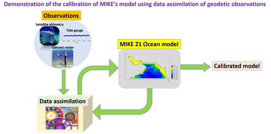
2.2. Methodology of Calibrating MIKE Model

The model used in this study was MIKE 21 with a flexible mesh. First, geometry and depth information must be introduced into the model. In addition to geometry and depth, the initial and boundary conditions of the model, including SLH and SSC data at the initial time, along with wind, precipitation, and evaporation data, should be added as inputs to the model. Geometry and depth information are among the most important information for ocean current modeling. A flexible meshing (without structure) was used to increase the accuracy of the calculations and reduce the computational time. For a more efficient calculation of the SSCs, a smaller mesh size in the islands and coastal strip (about 250 m) was selected. As fewer changes occur in offshore areas, larger mesh sizes were chosen (about 750 m) to speed up the performance. 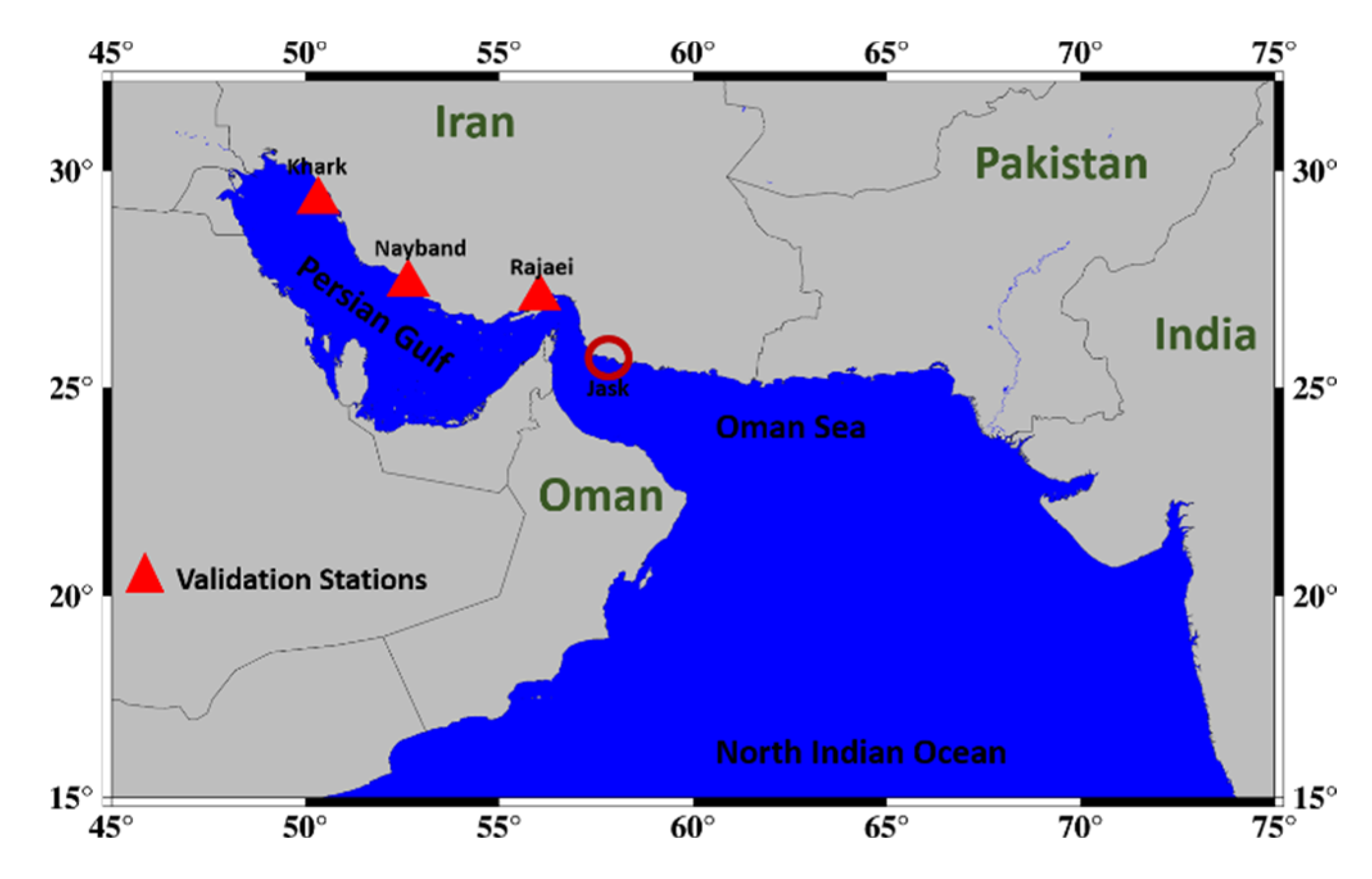For the initial conditions of the SLH and SSCs, the Copernicus Data Center, along with the MSS of the TM-IR01 model, were used (Table 4). The closed boundary conditions were introduced as zero velocity for the SSC components and the specified value for SLH. In fact, the SLH observations at the Chabahar, Rajaei, Khark, Karachi, and Misirah stations were used as boundary conditions for the closed boundary (Table 1). For open boundary conditions in the North Indian Ocean, the SLH was determined using the TM-IR01 tidal model (Table 1). TM-IR01 is a local tide model that is provided by the National Cartography Center (NCC) of Iran based on observations of three altimeters, including TOPEX/POSIDON, Jason1, and Jason 2, as well as 13 coastal tide gauge stations [26].

After creating the geometry and meshing of the model, as well as preparing the initial and boundary conditions, the following parameters should be considered in the MIKE 21 model [28,29]:

• Selecting the equation solution as “discretization of equations with high degrees”;
• Considering density as a function of temperature and salinity;
• Variable Coriolis force in place;
• Variable wind force;
• Tidal force by applying TM-IR01 model tidal components;
• Precipitation and evaporation;
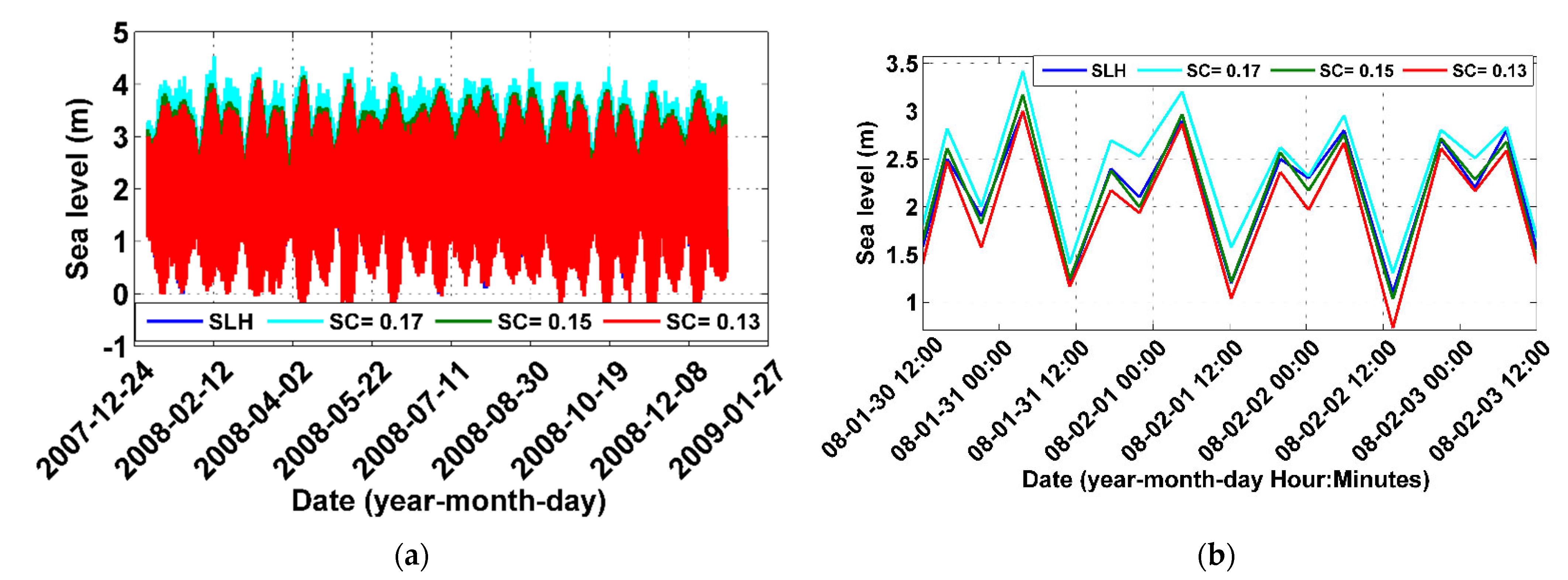
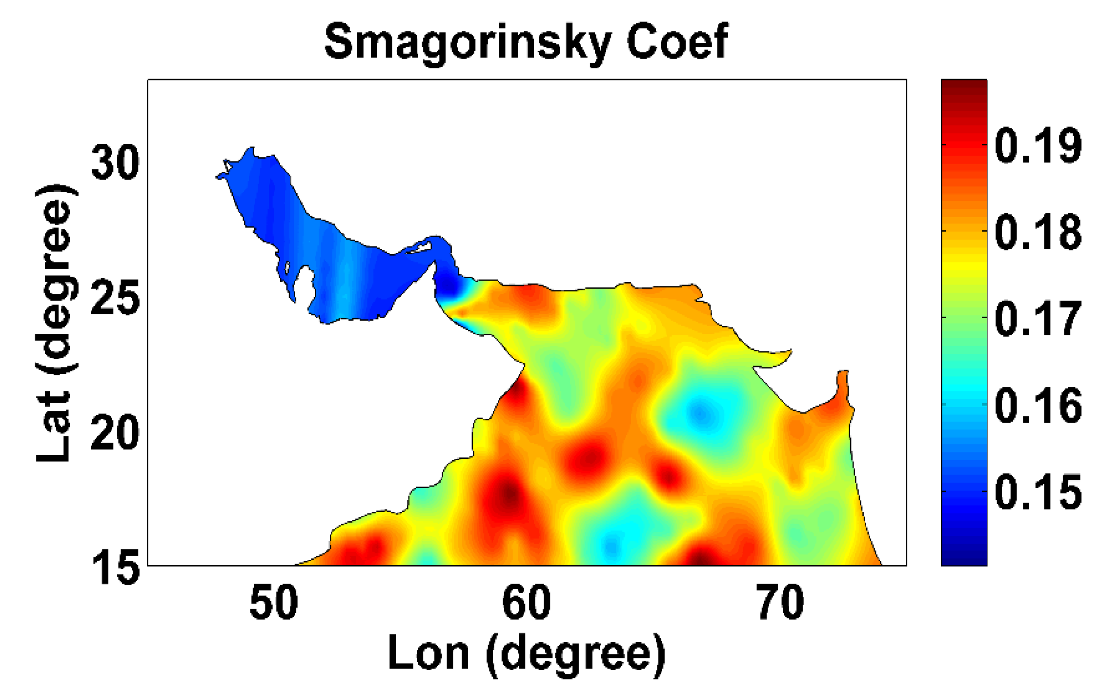
• The Smagorinsky formula was used for horizontal eddy viscosity [30], with a constant value of 0.28 for the Smagorinsky coefficient as the suggested number for the MIKE 21 model;
• In the MIKE 21 model, one of the most valuable features is the ability to dynamically adjust the domain of the computations. This enables one to calculate SSCs in areas that sometimes are dry and sometimes are wet, such as tidal zones;
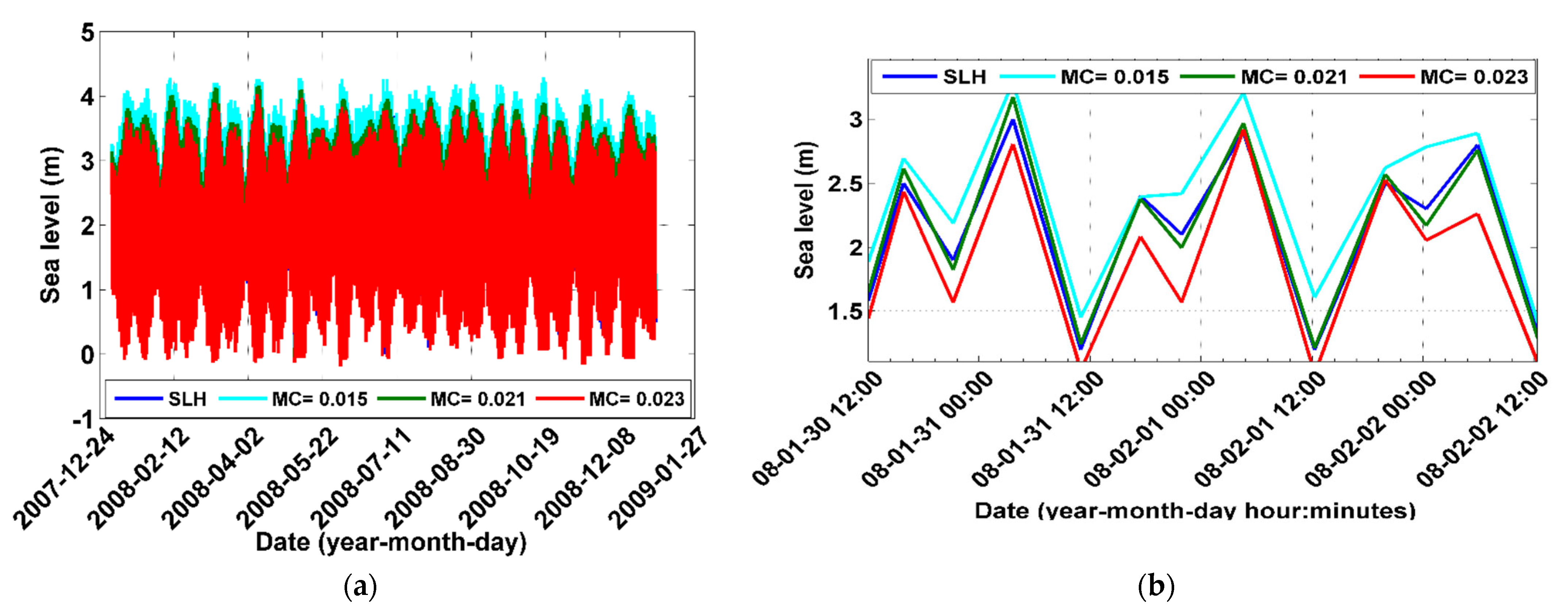
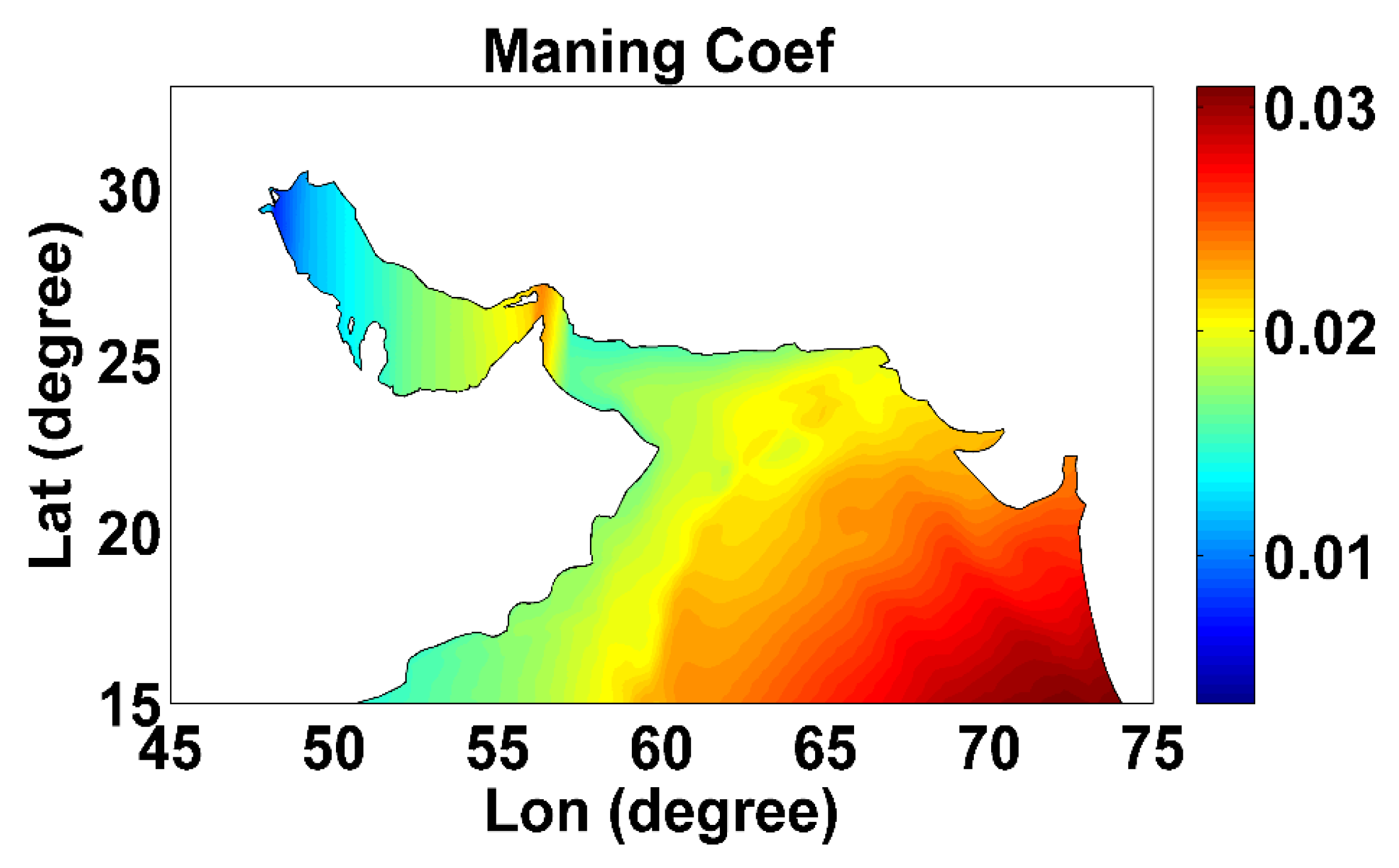
• Manning’s coefficient of 0.03 was applied for the bed resistance

After the above preparations, the time step for the numerical solution of the Navier–Stokes equation should be introduced into the program. This actually depends on the type of numerical method, as well as the dimensions and size of meshes used for discretization [31]. The interval chosen for the time step was between 0.01 and 1800 s in accordance with the stability criteria of the model, and the time step of running the model was 60 s.

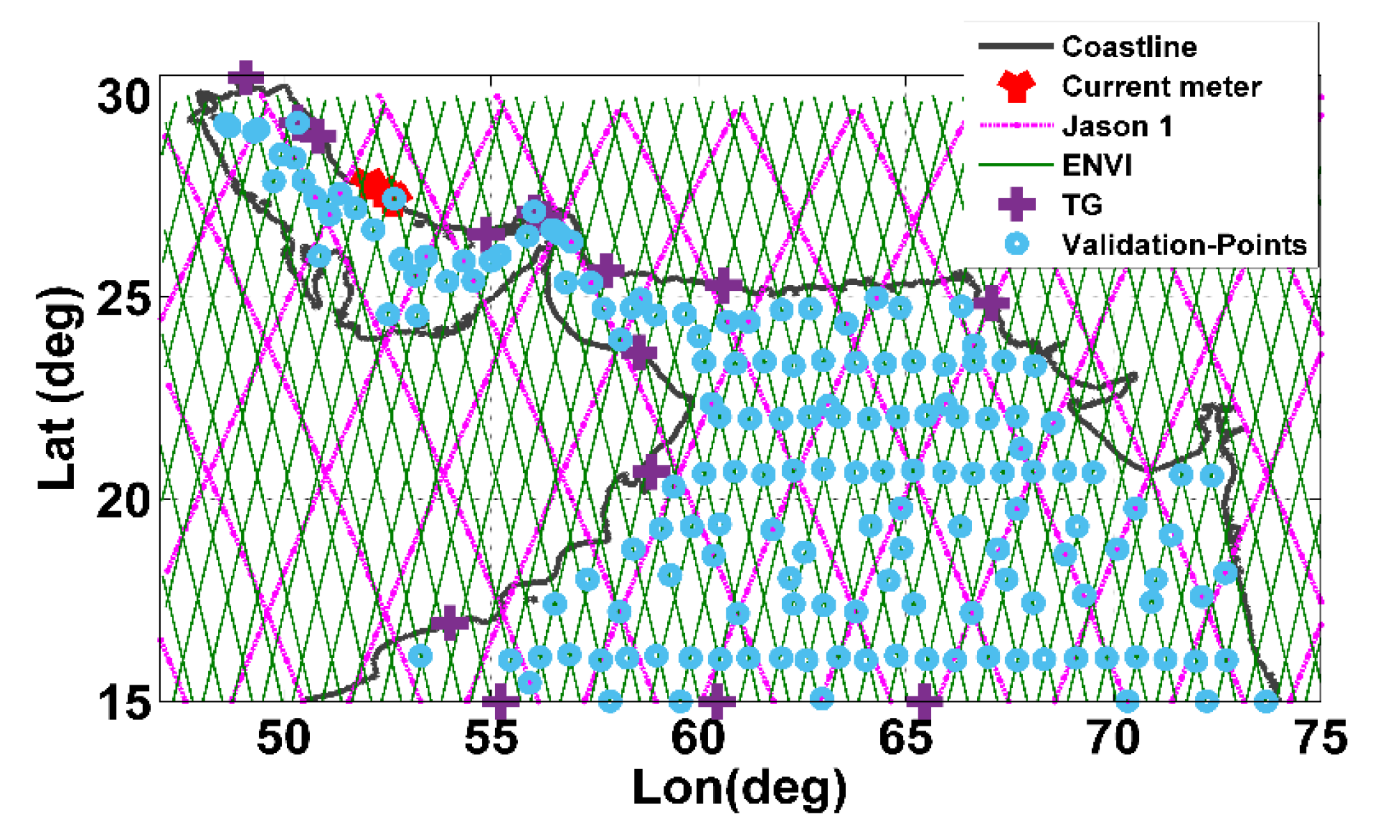
After introducing the required parameters into the MIKE 21 model, one could run the model to compute the SSCs and SLH. However, as it was discussed, here we tried to calibrate the model using a variational data assimilation procedure with the aid of local data, including coastal tide gauges (Table 1), current meters (Table 2), and satellite altimetry data (Table 3). In this case, a weighted objective function was defined, and that function was minimized using various optimization techniques [32]. The objective function J, based on the errors of force field (e_f), initial conditions (e_i), boundary conditions (e_b), in situ measurements (e), and the model (e_m), was defined as follows [33]:

$$\mathrm{J}(x^a{,\mathrm{F},\mathrm{I},\mathrm{B})=\mathrm{C}}_f{\underset{e_f}{\underbrace{(F-f)}}}^2+{\mathrm{C}}_i{\underset{e_i}{\underbrace{(I-i)}}}^2+{\mathrm{C}}_b{\underset{e_b}{\underbrace{(B-b)}}}^2+{\mathrm{C}}_y{\underset{e}{\underbrace{(y-H(x^m))}}}^2+C_m{\underset{e_m}{\underbrace{(x^a-x^m)}}}^2$$

(1)

In the above equation, F is the estimated force field, f is the initial force field (including the wind force, tides, and friction force parameters), C_f is the covariance matrix of the force field, I is the estimated initial conditions, i is the initial conditions (including the SLH and SSC components), C_i is the covariance matrix of the initial conditions, B is the estimated boundary conditions, b is the boundary conditions (including SLH data), C_b is the covariance matrix of the boundary conditions, y is the observations for data assimilation (including SLH and SSC components), H is the interpolation operator or observation operator, C_y is the covariance matrix of the data assimilation observations, x^a is the assimilated model, C_m is the covariance matrix of the model, and x^m is the output of the numerical model, including the SLH and SSC components derived from the MIKE model.

The error e_f may arise from errors in surface wind forcing. It may also arise from simplifications in equations of motion, such as hydrostatic approximation or parametrization of turbulent mixing. The initial and boundary errors (e_i and e_b) usually arise from errors in observation. Errors in the model occur due to discretization and numerical calculations, which have a solely mathematical nature [33].

In the next step, the covariance matrices for the force field (C_f) [33], initial and boundary conditions (C_i and C_b), observations (C_y), and model or background (C_m) were constructed. For the covariance matrix of the force field, including the covariance matrix of the wind (C_{Wind Force}), the covariance matrix of the tidal force (C_{Tidal Potential}), and the covariance matrix of the bed resistance (C_{Bed Resistance}), one could write:

$$C_f=\left[\begin{array}{ccc}{C}_{\mathrm{Wind} \mathrm{Force}}& 0& 0\\ 0& C_{\mathrm{Tidal} \mathrm{Potential}}& 0\\ 0& 0& C_{\mathrm{Bed} \mathrm{Resistance}}\end{array}\right]$$

(2)

Thus, we first needed to formulate the covariance matrix of the wind observations in the study area, which were in the form of a gridded time series. In addition, for C_{Tidal Potential}, we used the standard deviation of the tidal components, which were specified in the TM-IR01 model. The unit weight was considered for C_{Bed Resistance}. To this end, the covariance matrix of the wind was formed using a spatio-temporal empirical covariance function:

$$C_{\mathrm{Wind}}(\Delta \mathrm{s}, \Delta \mathrm{t})=\underset{C_s}{\underbrace{a{e}^{b\Delta s}}}\underset{C_{\mathrm{t}}}{\underbrace{c{e}^{d\Delta t}}}$$

in which a, b, c, and d are constant coefficients, and $\Delta \mathrm{s}, \Delta \mathrm{t}$ are the spatial and temporal steps, respectively [34].

In order to determine the covariance matrix of the initial conditions, which included the SLH observations (C_{sea level}) and the horizontal components of the SSC (C_u and C_v), (the initial conditions (SLH, u, and v) were in the form of a gridded file at the initial time), we used a spatial empirical covariance function (C_s) to determine the covariance of each observation [35]. Thus, one could write:

$$C_i=\left[\begin{array}{ccc}{C}_{\mathrm{sea} \mathrm{level}}& 0& 0\\ 0& C_u& 0\\ 0& 0& C_v\end{array}\right]$$

(3)

To form the covariance matrix of the boundary conditions (C_b in Equation (1)), we set C_b = C_TG, namely it was equal to the covariance matrix of the tide gauge observations. As it was discussed, the SLH observations from tide gauge stations were used as boundary conditions. To this end, for the covariance matrix of the tide gauge observations, the average of the SLH time series (MSL) was first subtracted from the SLH time series (SLA = SLH-MSL, which is a residual time series), and then its standard deviation was considered as the covariance matrix of the boundary conditions (C_b).

Finally, the covariance matrix of the observations in the data assimilation procedure, including satellite altimetry observations (C_{sea level ALT}), coastal tide gauge observations (C_{sea level TG}), and in situ current meter observations (C_u and C_v), was considered as follows:

$$C_y=\left[\begin{array}{cccc}{C}_{\mathrm{sea} \mathrm{level} \mathrm{ALT}}& 0& 0& 0\\ 0& C_{\mathrm{sea} \mathrm{level} \mathrm{TG}}& 0& 0\\ 0& 0& C_u& 0\\ 0& 0& 0& C_v\end{array}\right]$$

(4)

Since altimetry, tide gauge, and current observations were in the form of time series, matrices C_{sea level ALT,} C_{sea level TG}, C_u, and C_v could be formed by taking the standard deviation of their residual time series in a similar manner to explained for C_b. As it was seen, the computation of C_u and C_v for C_y was different from the computation of C_u and C_v for C_i.

Identifying the covariance matrix of the model or background was another challenge of the present study. During the data assimilation process, it is very important to have a correct estimation of this matrix. In situ observations are used to control how information from the model space is spread out by the components of the background covariance matrix [36]. In terms of size, when a model error is large, a greater weight is given to the data assimilation observations. In order to form the covariance matrix of a model, various methods have been proposed. In this study, the covariance matrix of the model was determined using the NMC method [37]. The variance–covariance matrix of the model was built through the comparison of 48 h forecasts of the model with 24 h forecasts of the model at a certain time (that is, using different initial and boundary conditions at different times for forecasting at the same specific time) [32]. Thus, one could write:

$$\begin{array}{l}{C}_m=\overline{\left(x^{48}-x^{24}\right){\left(x^{48}-x^{24}\right)}^T}\\ x^{48}=x^{True}+{\epsilon }^{48}+b^{48}\\ x^{24}=x^{True}+{\epsilon }^{24}+b^{24}\end{array}$$

(5)

In the above relation, x⁴⁸ and x²⁴ are, respectively, the 48 h and 24 h predictions of the model at a certain time; the upper bar indicates averaging over time or space; x_true is the correct value of the model (without error and bias); and ${\epsilon }^{48}$ and ${\epsilon }^{24}$ are the respective random errors. We also assumed that there was no bias or that the bias was constant over time (b⁴⁸ = b²⁴). As a result, the forecast difference could be expressed as follows [37]:

$$x^{diff}=x^{48}-x^{24}={\epsilon }^{48}-{\epsilon }^{24}$$

(6)

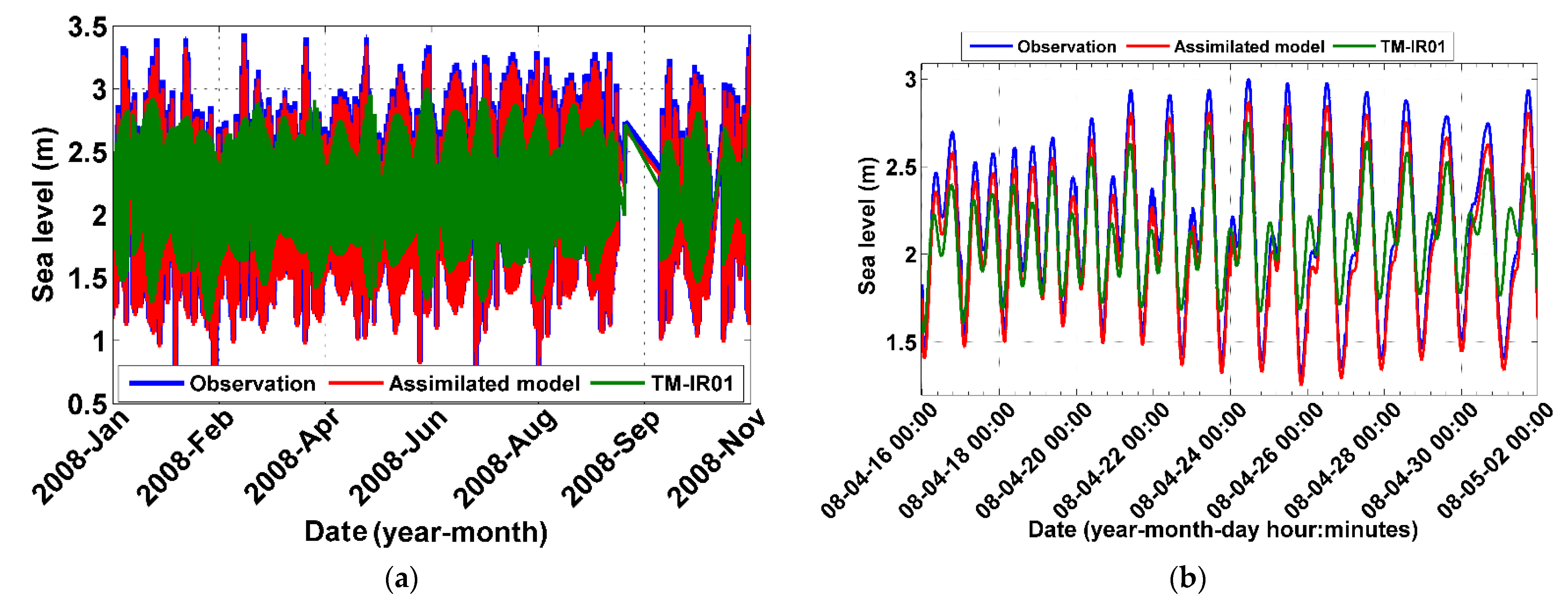
All of the above covariance matrices were considered as the initial values, and they were updated in an iterative way through the calibration and optimization procedures. In order to perform the process of calibration and data assimilation of the observations, we used MATLAB version 9.6 toolbox from the DHI company. This toolbox is able to link all output and input files of the MIKE 21 model to MATLAB software. In this way, by connecting the inputs and outputs of the MIKE model, the optimization process of the model was performed. MATLAB was used to create the objective function of Equation (1) in an iterative process by changing the input values of the MIKE model and rerunning the model until the model achieved acceptable accuracy [38].

3. Results

3.1. Numerical Ocean Model and Data Assimilation

In this section, the numerical results of the MIKE 21 model and data assimilation (calibration) procedure using metaheuristic optimization methods are presented. Figure 1 and Figure 2, for a typical example, show the SLH and horizontal SSC components before and after calibration of the model on 1 January 2008.

Three goals were pursued here: (i) choosing the appropriate optimization method for calibration; (ii) selecting the correct weights; and (iii) determining the effect of the defined objective function on the results. For the first goal, the performance of each optimization method was evaluated following the assimilation of coastal tide gauge and current meter data. Comparisons were made between the assimilated model, the coastal tide gauges, and the current meter observations, both with and without the variance covariance matrices of the objective functions (Equation (1)). In Figure 3, the mean correlation coefficient and root mean square error (RMSE) are depicted for each optimization method in all the tide gauge stations (except control stations) and current meter stations (except control stations), respectively, with and without considering the variance–covariance matrices. The results of this study indicate that, in general, the GA and TLBO methods provided better performances (more correlation and fewer errors compared to local data) than the PSO and SCE methods. In addition, considering the variance–covariance matrices increased the correlation between the assimilated model and local data. Particularly, the correlation coefficients between the assimilated model and coastal tide gauge observations, respectively, in the GA, PSO, TLBO, and SCE methods without considering the variance–covariance matrices were equal to 0.66, 0.58, 0.65, and 0.55; by considering them, they were equal to 0.82, 0.75, 0.87, and 0.69. The correlation coefficients between the assimilated model and the current meter observations, both without considering the variance–covariance matrices and considering them in the GA, PSO, TLBO, and SCE methods, were equal to 0.71, 0.68, 0.72, and 0.64 and 0.85, 0.79, 0.83, and 0.71, respectively.

Further investigation of the performances of the mentioned optimization methods was provided by comparing the assimilated model with those of the control stations at coastal tide gauge (Rajaei and Khark) and current meter stations (Nayband station). In the GA, PSO, TLBO, and SCE methods, the RMSE values between the assimilated model and the two control stations (Rajaei and Khark) were equal to 0.082, 0.090, 0.071, and 0.11 m and 0.091, 0.10, 0.086, and 0.13 m, respectively. For the east–west component of the SSC, the RMSE values were equal to 0.084, 0.088, 0.069, and 0.097 m/s, while for the north–south component, they were equal to 0.081, 0.085, 0.073, and 0.10 m/s. As a typical example, Figure 4 illustrates the estimation of the SLH at the Rajaei tide gauge station using each of the optimization methods. According to the obtained results, the TLBO method performed better than the other methods.

For the second goal, the effect of the variance–covariance matrices (Equation (1)) on data assimilation was investigated. To this end, the process of data assimilation was performed once considering the variance–covariance matrices and then without considering the variance–covariance matrices (unit weight). When the variance–covariance matrices were used, the correlation between the observations and the assimilated model increased, and the assimilated model became closer to the observed data. Figure 5, for a typical example, shows the correlations between the SLH observations at the Rajaei tide gauge station and the model in three cases: (a) before data assimilation, (b) after data assimilation without considering the variance–covariance matrices, and (c) considering the variance–covariance matrices. Figure 6, for a typical example, shows the correlations between the horizontal SSC components (u, v) at the Taheri current meter station and the model in three cases similar to those in Figure 5.

For the third goal, to further investigate the objective function (Equation (1)) and the performances of the variance–covariance matrices, each variance–covariance matrix was applied separately during the data assimilation process.

Table 5. RMSE values between the assimilated (calibrated) model and tide gauge observations at Rajaei and Khark control stations and current meter observation at Nayband control station.

	Different State of Objective Function
Observations	$\begin{array}{l}{\mathrm{C}}_f={\mathrm{C}}_f;\\ {\mathrm{C}}_i={\mathrm{C}}_i;\\ {\mathrm{C}}_b={\mathrm{C}}_b;\\ {\mathrm{C}}_y={\mathrm{C}}_y;\\ C_m=C_m;\end{array}$	$\begin{array}{l}{\mathrm{C}}_f={\mathrm{C}}_f;\\ {\mathrm{C}}_i={\mathrm{C}}_i;\\ {\mathrm{C}}_b={\mathrm{C}}_b;\\ {\mathrm{C}}_y={\mathrm{C}}_y;\\ C_m=I;\end{array}$	$\begin{array}{l}{\mathrm{C}}_f={\mathrm{C}}_f;\\ {\mathrm{C}}_i={\mathrm{C}}_i;\\ {\mathrm{C}}_b={\mathrm{C}}_b;\\ {\mathrm{C}}_y=I;\\ C_m=I;\end{array}$	$\begin{array}{l}{\mathrm{C}}_f={\mathrm{C}}_f;\\ {\mathrm{C}}_i={\mathrm{C}}_i;\\ {\mathrm{C}}_b=I;\\ {\mathrm{C}}_y=I;\\ C_m=I;\end{array}$	$\begin{array}{l}{\mathrm{C}}_f={\mathrm{C}}_f;\\ {\mathrm{C}}_i=I;\\ {\mathrm{C}}_b=I;\\ {\mathrm{C}}_y=I;\\ C_m=I;\end{array}$	$\begin{array}{l}{\mathrm{C}}_f=I;\\ {\mathrm{C}}_i=I;\\ {\mathrm{C}}_b=I;\\ {\mathrm{C}}_y=I;\\ C_m=I;\end{array}$
SLH at Rajaei station (meter)	0.071	0.079	0.087	0.098	0.118	0.124
SLH at Khark station (meter)	0.086	0.091	0.097	0.109	0.127	0.132
The east–west component of SSC at Nayband station (U) (meters per second)	0.069	0.076	0.088	0.091	0.105	0.114
The north–south component of SSC at Nayband station (V) (meters per second)	0.073	0.087	0.094	0.103	0.110	0.119

shows the root mean square error (RMSE) values between the assimilated model (calibrated model) and the observations at control stations, including the SLH at the Rajai and Khark stations and the SSC at the Nayband station. According to the obtained results, the errors between the observations and assimilated models were reduced when all the variance–covariance matrices were used. As shown in this issue, applying each of the variance–covariance matrices improved the data assimilation process.

3.2. Validation and Control of Calibrated Model

As part of the validation process, we used control stations that were not involved in the modeling and data assimilation process. Figure 7 shows the validation stations and the names of the areas that are mentioned in this section. In order to control the calibrated model, the Nayband current meter station, Rajai tide gauge, and Khark tide gauge were used, along with satellite altimetry observations (167 points). It should be mentioned that satellite altimetry observations were used for both data assimilation and control of the results (validation). As shown in Figure 8, the study area included control points of two missions of satellite altimetry passes, as well as coastal tide gauges and in situ current meters. The RMSE values between the assimilated model and the observations of control stations at the Rajai and Khark coastal tide gauges were, respectively, 0.071 m and 0.086 m; at the Nayband current meter station, the values were 0.069 m/s for the east–west component and 0.073 m/s for the south–north component. Comparing the RMSE values before and after assimilation showed that the assimilation led to an improvement of about 0.09 m/s in the SSC of the Nayband control station and about 0.25 and 0.37 m in the SLH of the Rajai and Khark control stations, respectively. In addition, the RMSE values between the assimilated model and the satellite altimetry observations at control stations varied between 0.058 and 0.085 m. Moreover, the RMSE values between satellite altimetry observations and the assimilated model at the control points varied between 0.058 and 0.085 m. A typical example is shown in Figure 9, which illustrates SLH observations at the Rajaei control station and current meter observations at the Nayband control station, as well as for the model before and after data assimilation.

In addition, the effect of the Manning bed resistance coefficient, the Smagorinsky turbulence coefficient, and the amplitude and phase of the tidal components on SLH were studied in order to examine the effect of data assimilation in the calibration of the SSC model. There was a difference between the model and the observations when the Manning and Smagorinsky coefficients were applied incorrectly, as well as the amplitude and phase of tidal components. Figure 10 shows the performances of Manning coefficients of 0.015, 0.021, and 0.023 at the Rajaei control station and their effects on SLH. The optimal coefficient at this station was 0.021. Figure 11 illustrates the optimal Manning coefficient in the study area. Figure 12 shows the performances of Smagorinsky coefficients of 0.13, 0.15, and 0.17 at the Rajaei control station and their effects on SLH, and the optimal coefficient for this station was equal to 0.15. Figure 13 shows the optimal Smagorinsky coefficient in the study area, which had smooth variations in the Persian Gulf.

Regarding tidal components, the TM-IR01 model was used to calculate a tidal potential for MIKE 21. The results of the TM-IR01 model have already been validated with global tide models, such as the FES tide model [26]. Here, after data assimilation, we were looking for whether the tidal components of the TM-IR01 model were improved or not. The answer was yes. The amplitude and phase of the tidal components of this model were improved. To show this, with the aid of an empirical tide model (Equation (7)) [39], a comparison between the TM-IR01 tidal model and the calibrated (assimilated) model was conducted; to achieve this, an SLH time series of the tide gauge stations was reconstructed using tidal components of both the TM-IR01 and assimilated models, and then the differences between the tide gauge observations and both reconstructed SLH time series were calculated for RMSE computation.

$$SLH\left(t\right)=MSL+{\displaystyle \sum _{k=1}^m{A}_k\cos \left(2\pi f_{k}t+{\phi }_k\right)}$$

(7)

In this equation, SLH is the sea level height observed, MSL is the mean sea level, A_k is the amplitude of the tidal components, F_K is the frequency of the tidal components, ${\phi }_k$ is the phase of the tidal components, and m is the number of tidal frequencies. As an example, Figure 14 shows the SLH observation at Khark station and the reconstruction of the time series using the TM-IR01 and assimilated models.

Table 6. RMSE results between SLH of tide gauge stations and TM-IR01 model, as well as assimilated model.

Station	TM-IR01 Model	Assimilated Model
Muscat	0.121	0.081
Masirah	0.112	0.084
Salalah	0.126	0.097
Karachi	0.109	0.078
Khark	0.132	0.094
Jask	0.113	0.081
Chabahar	0.132	0.075
Rajaei	0.129	0.088
Lengeh	0.115	0.079
Khomeini	0.127	0.082
Bushehr	0.131	0.081
Bahman	0.127	0.086

shows the RMSE results between the tide gauge stations and TM-IR01 model, as well as the assimilated model.

3.3. Analyzing the Results of the SSC and Its Application in Producing Renewable Energy

The relevant analysis was based on data from 1 January 2008 to 1 January 2009 since the modeling was performed during this period. As a typical example, Figure 15 illustrates the SSCs in the Persian Gulf and the Oman Sea after data assimilation (assimilated or calibrated model) on 1 January 2008. Following the assimilated model showed that the SSC pattern changed in different areas, and it became closer to in situ observations through comparison with the model before assimilation. There were, primarily, three sources of SSCs in the Persian Gulf: density, wind, and tides. However, the main and most important SSC in the Persian Gulf was the cyclonic eddy that occurred when seawater entered the Persian Gulf from the Oman Sea (Figure 15). According to this pattern of SSC, the Persian Gulf had a higher salinity than the Oman Sea. Through the Strait of Hormuz, seawater with typical ocean salinity entered the Persian Gulf and moved northwest, parallel to the coast of Iran, and then changed direction to the south in the western part of the basin. During travel along this route, the water became denser, and its salinity increased as a result of evaporation, and finally, after traveling the southern portions, this SSC became denser and exited the Strait of Hormuz.

As a result of the changes in various parameters, density was the dominant parameter in the northern and central parts of the Persian Gulf. SSCs caused by the wind dominated the northwestern part of the Persian Gulf. Figure 16 shows a typical example of the difference in density of seawater on 1 January 2008 03:00 a.m. This difference was the difference between the density of seawater and water (density of seawater (kg/m³)—1000 (kg/m³)).

In addition, the range of tidal currents in the Persian Gulf is large, and their amount exceeds one meter at all times. In the area of the Tonb-Bozorg and Tonb-Kochak Islands, as well as the Abu Musa Island, the average SSCs in different months of the year showed the formation of eddies in the eastern and western parts of the Strait of Hormuz. In a similar manner to [40], water entered the Persian Gulf from the northern part of the Strait of Hormuz and spread along the northern coast. The SSC speed in the Strait of Hormuz was typically between 0.12 and 0.25 m/s, which is consistent with a previous study by [40]. It was common to see various eddies in the Oman Sea in the north and northwest (Pakistan and Iran), west (along the coasts of Oman), east (along the coasts of India), and in the North Indian Ocean. These eddies were caused by the factors mentioned above.

To investigate the SLH fluctuations in the Persian Gulf and the Oman Sea, the four main tidal components of M2, S2, K1, and O1 were considered. These four main components were applied to the model, and two different modes were considered: (1) adding wind data and considering density; and (2) not adding wind data and considering density. As can be seen from the results, tides dominated the SSCs of the Persian Gulf and the Oman Sea. According to the results, tidal currents accounted for a much higher proportion of currents (more than 70%) than other factors causing currents (winds and density variations). As a result of the great depth of the Oman Sea, the tidal currents were slower than those in the Persian Gulf. Thus, the areas adjacent to the Oman Sea had lower speeds and ranges of SSCs.

Over the last few decades, researchers around the world have focused their attention on marine renewable energy. It is known that Iran has a long coastline and that there are both permanent and momentary SSCs with different speeds and directions. Thus, with the aid of kinetic energy created by SSCs, they can be used as a renewable energy source. In order to accomplish this, coastal areas where kinetic energy is present in significant amounts are initially identified, and then equipment with different turbines is installed to convert this energy into electricity. It was previously possible to produce 100 watts of electricity from an SSC with a current speed of 1.2 m/s, but today, this capability can be provided by an SSC with a speed of 60 to 80 cm per second [41]. In this study, we also identified areas in the Persian Gulf and the Oman Sea that were likely to be utilized to produce electrical energy from the kinetic energy of SSCs. The following equation was used to calculate the kinetic energy of sea currents during 2008–2009 [42]:

$$\overline{u}=\frac{1}{N}{\displaystyle \sum _{k=1}^N{u}_k},\hspace{0.17em}\hspace{0.17em}\hspace{0.17em}\hspace{0.17em}\overline{v}=\frac{1}{N}{\displaystyle \sum _{k=1}^N{u}_v}\hspace{0.17em}\hspace{0.17em}\hspace{0.17em}\hspace{0.17em},E=\frac{{\overline{u}}^2+{\overline{v}}^2}{2}$$

(8)

In the above relation, $\overline{u}$ and $\overline{v}$ are, respectively, the mean SSC components in the east–west and north–south directions, and E is the mean kinetic energy caused by the SSC. Figure 17 shows the mean kinetic energy in the study area. In the Oman Sea and near Jask port, it was possible to use the kinetic energy of the currents. In this context, it is important to note that the obtained kinetic energy values were acceptable based on the estimation of the error of the SSC components using in situ data (Table 5).

4. Discussion

The Persian Gulf and the Oman Sea are strategically important regions where petroleum energy is transported from this region to other parts of the world. Therefore, the study of surface currents in this region is crucial for better understanding of the regional climate, the environment, and maritime transportation, as well as movements of oil and non-oil pollution. In the oceanic domain, numerical ocean circulation models have generally been used to solve initial boundary-value problems. In the absence of knowledge regarding parameters and boundary values, they may suffer from calibration concerns, and their results may not be accurate enough for local and regional applications, and they may also require local tuning (calibration) to be accurate.

In this study, we calibrated MIKE 21 for the computation of SSCs. As a result of this approach, we encountered three main challenges: (1) selecting the correct objective functions, (2) appropriately tuning the weights of the objective functions, and (3) selecting an appropriate method to optimize the objective functions. To deal with these challenges, the following novelties and innovations were considered in this manuscript

(i): A comprehensive calibration of the MIKE 21 numerical ocean model was conducted over the Persian Gulf and the Oman Sea via data assimilation with satellite altimetry and hydrographic observations. The calibration dealt with errors of input data, such as errors of boundary and initial conditions, as well as uncertainties of some model parameters, such as Smagorinsky and Manning coefficients or bed resistance information. It also considered the intrinsic errors arising from the numerical solution to the Navier–Stokes equation.

(ii): A novel optimization problem was defined to assimilate in situ data with the MIKE 21 model via minimization of all possible errors in the modeling process. It was a multiobjective optimization scheme that is solved using metaheuristic algorithms, such as genetic algorithms (GAs), particle swarm optimization (PSO), teaching-learning-based optimization (TLBO), and shuffled complex evolution (SCE).

(iii) To deal with one of the important issues in the multiobjective calibration regarding the definition of proper weight functions, in this study, a simple method based on the types of observations and the statistical methods was suggested to resolve this problem, and its effectiveness and performance were illustrated using different examples.

(iv) We also faced the challenge of lacking low-spatial-resolution data from tide gauges and current meters. Therefore, we decided to use satellite altimetry data in the assimilation, which is a comprehensive and reliable source of information for the study of ocean and sea level variations.

(v) As a result of the proposed method, the SSC and SLH estimations in the Persian Gulf and the Oman Sea were demonstrated with a reasonable degree of accuracy, and this approach could be easily adopted to other areas. Moreover, as an interesting and feasible application of this study, the kinetic energy caused by the SSCs was determined using the calibrated model, and it was analyzed to identify areas that were prone to be used for the generation of electricity from SSCs.

5. Conclusions

In this study, the MIKE 21 two-dimensional hydrodynamic model with flexible mesh was used for modeling SSCs in the Persian Gulf and the Oman Sea. The above model was in operation for one year. After defining the weighted objective function, the data assimilation was performed by minimizing the function using optimization methods, such as GA, PSO, TLBO, and SCE. In a final step, the kinetic energy associated with SSCs was determined using the assimilated model. Generally, data assimilation improved the estimation of the SSC components, based on the results of the data assimilation procedure. Based on the assimilated model, the RMSE values between the coastal tide gauges at the Rajaei and Khark control stations and the current meter at the Nayband control station were 0.071 m and 0.086 m, as well as 0.069 m/s for the east–west SSC component and 0.073 m/s for the north–south SSC component, respectively. Moreover, the RMSE values between satellite altimetry observations and the assimilated model at the control points varied between 0.058 and 0.085 m. Furthermore, the appropriate application of variance–covariance matrices increased the accuracy of estimating the SLH and SSC components. In addition, the GA and TLBO optimization methods provided better results than PSO and SCE. According to the results of the optimal estimation of the bed friction coefficient, as well as the Smagorinsky turbulence coefficient, the bed friction coefficient had a significant effect on the variation in the SLH and SSC components in the Persian Gulf and Oman Sea. This variation may be due to the increasing depth in the Persian Gulf and the Oman Sea. Moreover, the amplitude and phase of the tidal components were reconstructed before and after data assimilation using an empirical tide model, which was tested with the Khark tide gauge control station and indicated that the amplitude and phase of the assimilated model were accurate. Further, it was possible to utilize the kinetic energy of sea currents in the Oman Sea and near the port of Jask by examining the kinetic energy created by the SSCs in the Persian Gulf and Oman Sea. Moreover, it was shown that the SSC pattern changed in different areas after data assimilation, becoming more similar to the in situ observations in the Persian Gulf and Oman Sea. According to the SSC pattern of the Strait of Hormuz, the SSC moved from the Oman Sea toward the Persian Gulf. Due to the difference in density between the Oman Sea and the Persian Gulf, a cyclonic eddy formed in the Persian Gulf. In the Persian Gulf, coastal currents were primarily caused by tides, but in the Oman Sea and the North Indian Ocean, near Pakistan, India, and Oman, eddies were created resulting from changes in density, wind, and bathymetry.

In the context of expanding future research in this field, other sources of data, such as sea surface temperature and sea surface salinity, could be used in the calibration process. In addition, the proposed data assimilation method should be tested on other numerical ocean models. Furthermore, it is possible to check areas prone to the use of marine energy in the study area with the aid of wave modeling.

References

1. Dauji, S.; Deo, M.; Bhargava, K. Prediction of ocean currents with artificial neural networks. J. Hydraul. Eng. 2014, 21, 14–27. [Google Scholar] [CrossRef]
2. Saha, D.; Deo, M.C.; Joseph, S.; Bhargava, K. A combined numerical and neural technique for short term prediction of ocean currents in the Indian Ocean. Environ. Syst. Res. 2016, 5, 4. [Google Scholar] [CrossRef]
3. Sadrinasab, M. Three-dimensional flushing times of the Persian Gulf. Geophys. Res. Lett. 2004, 31, L24301. [Google Scholar] [CrossRef]
4. Shchepetkin, A.; McWilliams, J. The regional oceanic modeling system (ROMS): A split-explicit free-surface topography-following-coordinate oceanic model. Ocean Model. 2005, 9, 347–404. [Google Scholar] [CrossRef]
5. Bryan, K. A Numerical Method for the Study of the Circulation of the World Ocean. J. Comput. Phys. 1997, 135, 154–169. [Google Scholar] [CrossRef]
6. Saputra, R.A.; Perdanawati, R.A.; Akhwadhy, R. Hydrodynamic modelling using software of MIKE 21 in the land reclamation of Jakarta Bay. Current condition and master plan. In Proceedings of the Built Environ Sci Technol International Conference, Surabaya, Indonesia, 18–19 September 2018. [Google Scholar] [CrossRef]
7. Chao, S.; Kao, T.W.; Al-Hajri, K.R. A numerical investigation of circulation in the Arabian Gulf. J. Geophys. Res. 1992, 97, 11219–11236. [Google Scholar] [CrossRef]
8. Saberi Najafi, S. Modeling Tide in Persian Gulf Using Dynamic Nesting. Ph.D. Thesis, University of Adelaide, Melbourne, Australia, 1997. [Google Scholar]
9. Blain, C.A. Modeling three-dimensional thermohaline-driven circulation in the Arabian Gulf. In Estuarine and Coastal Modeling, Proceedings of the 6th International Conference, Stanford, CA, USA, 14–16 August 2000; American Society of Civil Engineers: Reston, VA, USA, 2000; pp. 74–92. [Google Scholar]
10. Kämpf, J.; Sadrinasab, M. The circulation of the Persian Gulf: A numerical study. Ocean Sci. Discuss. 2005, 2, 129–164. [Google Scholar] [CrossRef]
11. Sabbagh-Yazdi, S.R.; Zounemat-Kermani, M.; Kermani, A. Solution of depth averaged tidal currents in Persian Gulf on unstructured overlapping finite volumes. Int. J. Numer. Methods Fluids 2007, 55, 81–101. [Google Scholar] [CrossRef]
12. Afshar-Kaveh, N.; Ghaheri, A.; Chegini, V.; Etemad-Shahidi, A.; Nazarali, M. Evaluation of different wind fields for storm surge modeling in the Persian Gulf. J. Coast. Res. 2017, 333, 596–606. [Google Scholar]
13. Bertino, L.; Evensen, G.; Wackernagel, H. Sequential Data Assimilation Techniques in Oceanography. Int. Stat. Rev. 2007, 71, 223–241. [Google Scholar] [CrossRef]
14. Peng, S.; Xie, L.; Pietrafesa, L.J. Correcting the errors in the initial conditions and wind stress in storm surge simulation using an adjoint optimal technique. Ocean Model. 2007, 18, 175–193. [Google Scholar] [CrossRef]
15. Zalesny, V.; Agoshkov, V.; Shutyaev, V.; Parmuzin, E.; Zakharova, N. Numerical modeling of marine circulation with 4D variational data assimilation. J. Mar. Sci. Eng. 2020, 8, 503. [Google Scholar] [CrossRef]
16. Sirkes, Z.; Tziperman, E.; Thacker, W. Combining data and a global primitive equation ocean general circulation model using the adjoint method. Elsevier Oceanogr. 1996, 61, 119–145. [Google Scholar] [CrossRef]
17. Mayo, T.; Butler, T.; Dawson, C.; Hoteit, I. Data assimilation within the advanced circulation (ADCIRC) modeling framework for the estimation of manning’s friction coefficient. Ocean Model. 2014, 76, 43–58. [Google Scholar] [CrossRef]
18. Stammer, D.; Ray, R.D.; Andersen, O.B.; Arbic, B.K.; Bosch, W.; Carrere, L.; Cheng, Y.; Chinn, D.S.; Dushaw, B.D.; Egbert, G.D. Accuracy assessment of global barotropic ocean tide models. Rev. Geophys. 2014, 52, 243–282. [Google Scholar] [CrossRef]
19. Vrugt, J.A.; Gupta, H.V.; Bastidas, L.A.; Bouten, W.; Sorooshian, S. Effective and efficient algorithm for multiobjective optimization of hydrologic models. Water Resour. Res. 2003, 39, 8. [Google Scholar] [CrossRef]
20. Lakshmi, V.R. Optimization of thinned dipole arrays using genetic algorithm. Int. J. Eng. Technol. 2011, 3, 658–662. [Google Scholar] [CrossRef]
21. Gao, Y.; Zhu, K. Hybrid PSO-solver algorithm for solving optimization problems. J. Comput. Appl. 2012, 31, 1648–1651. [Google Scholar] [CrossRef]
22. Rao, R.V. Optimization of multiple chiller systems using TLBO algorithm. In Teaching Learning Based Optimization Algorithm; Springer: Cham, Germany, 2016; pp. 115–128. [Google Scholar] [CrossRef]
23. Sivamathi, C.; Vijayarani, S. Assimilation high utility itemsets using shuffled complex evolution of particle swarm optimization (SCE-PSO) optimization algorithm, 2017. In Proceedings of the International Conference on Inventive Computing and Informatics (ICICI), Coimbatore, India, 23–24 November 2017. [Google Scholar] [CrossRef]
24. Yang, X.S. Metaheuristic Optimization. Scholarpedia 2011, 6, 11472. [Google Scholar] [CrossRef]
25. Zhang, G.; Pan, L.; Neri, F.; Gong, M.; Leporati, A. Metaheuristic Optimization: Algorithmic Design and Applications. J. Optim. 2017, 2017, 1053145. [Google Scholar] [CrossRef]
26. Soltanpour, A.; Pirooznia, M.; Aminjafari, S.; Zareian, P. Persian Gulf and Oman sea tide modeling using satellite altimetry and tide Gauge data (TM-IR01). Mar. Georesour. Geotechnol. 2017, 36, 677–687. [Google Scholar] [CrossRef]
27. Hall, J.K. GEBCO Centennial special issue—Charting the secret world of the ocean floor. The GEBCO project 1903–2003. Mar. Geophys. Res. 2006, 27, 1–5. [Google Scholar] [CrossRef]
28. Wang, Q.; Peng, W.; Dong, F.; Liu, X.; Ou, N. Simulating flow of an urban river course with complex cross sections based on the MIKE 21 FM model. Water 2020, 12, 761. [Google Scholar] [CrossRef]
29. Manson, G.K. Configuration of MIKE 21 for the simulation of nearshore storm waves currents and sediment transport: Brackley bight Prince Edward Island. Geol. Surv. Can. 2012. [Google Scholar] [CrossRef]
30. Uddin, M.; Mallik, M. Large eddy simulation of turbulent channel flow using Smagorinsky model and effects of Smagorinsky constants. Br. J Math. Comp. Sci. 2015, 7, 375–390. [Google Scholar] [CrossRef]
31. Russell, T.F. Stability Analysis and Switching Criteria for Adaptive Implicit Methods Based on the CFL Condition; SPE Symposium on Reservoir Simulation: Houston, TX, USA, 1989. [Google Scholar]
32. Zalesny, V.B.; Agoshkov, V.I.; Shutyaev, V.P.; Le Dimet, F.; Ivchenko, B.O. Numerical modeling of ocean hydrodynamics with variational assimilation of observational data. Izv.-Atmos. Ocean. Phys. 2016, 52, 431–442. [Google Scholar] [CrossRef]
33. Chua, B.; Bennett, A. An inverse ocean modeling system. Ocean Model. 2001, 3, 137–165. [Google Scholar] [CrossRef]
34. Mariella, L.; Tarantino, M. Spatial temporal conditional auto-regressive model: A new autoregressive matrix. Austrian J. Stat. 2016, 39, 223–244. [Google Scholar] [CrossRef]
35. Pirooznia, M.; Raoofian Naeeni, M. The application of least-square collocation and variance component estimation in crossover analysis of satellite altimetry observations and altimeter calibration. J. Oper. Oceanogr. 2020, 13, 100–120. [Google Scholar] [CrossRef]
36. Lee, J.C.; Huang, X. Modelling the Background Error Covariance Matrix: Applicability Over the Maritime Continent. In Data Assimilation for Atmospheric, Oceanic and Hydrologic Applications; Park, S.K., Xu, L., Eds.; Springer: Cham, Germany, 2021; Volume IV, pp. 599–627. [Google Scholar] [CrossRef]
37. Wang, H.; Huang, X.; Sun, J.; Xu, D.; Zhang, M.; Fan, S.; Zhong, J. Inhomogeneous background error modeling for WRF-Var using the NMC method. J. Appl. Meteorol. Climatol. 2014, 53, 2287–2309. [Google Scholar] [CrossRef]
38. DeChant, C. Hydrologic data assimilation: State estimation and model calibration. In Dissertations and Theses; Portland State University ProQuest Dissertations Publishing: Portland, OR, USA, 2000; p. 172. [Google Scholar] [CrossRef]
39. Pirooznia, M.; Emadi, S.R.; Alamdari, M.N. The time series spectral analysis of satellite altimetry and coastal tide gauges and tide modeling in the coast of Caspian Sea. Open J. Mar. Sci. 2016, 6, 258–269. [Google Scholar] [CrossRef]
40. Thoppil, P.G.; Hogan, P.J. A modeling study of circulation and eddies in the Persian Gulf. J. Phys. Oceanogr. 2010, 40, 2122–2134. [Google Scholar] [CrossRef]
41. Dudhgaonkar, P.; Duraisamy, N.; Jalihal, P. Energy extraction from ocean currents using straight bladed cross-flow hydrokinetic turbine. Int. J. Ocean. Clim. Syst. 2017, 8, 4–9. [Google Scholar] [CrossRef]
42. Shenoi, S.S.; Saji, P.K.; Almeida, A.M. Near-surface circulation and kinetic energy in the tropical Indian Ocean derived from lagrangian drifters. J. Mar. Res. 1999, 57, 885–907. [Google Scholar] [CrossRef]
Figure 1. (a) Sea level height before data assimilation (calibration); (b) east–west component (u) of the SSC before data assimilation; (c) north–south component (v) of the SSC before data assimilation.
Remotesensing 14 04901 g001
Figure 2. (a) Sea level height after data assimilation (calibration); (b) east–west component (u) of the SSC after data assimilation; (c) north–south component (v) of the SSC after data assimilation.
Remotesensing 14 04901 g002
Figure 3. (a) The performance of each optimization method at tide gauge stations with and without considering covariance matrices. (b) The performance of each optimization method at current meter stations with and without considering covariance matrices.
Remotesensing 14 04901 g003aRemotesensing 14 04901 g003b
Figure 4. SLH at Rajaei tide gauge station using different optimization methods.
Remotesensing 14 04901 g004
Figure 5. Correlations between the observations of the SLH at the Rajaei tide gauge station and the model output in three cases: (a) before data assimilation, (b) after data assimilation without considering the variance–covariance matrices, and (c) considering the variance–covariance matrices.
Remotesensing 14 04901 g005
Figure 6. The correlations between the east–west component (u) of the SSC at Taheri current meter station and the model in three cases: (a) before data assimilation (calibration), (b) after data assimilation without considering the variance–covariance matrices, and (c) after considering the variance–covariance matrices. The correlations between the observations of the north–south component (v) of the SSC at the Taheri current meter station and the model in three cases: (d) before data assimilation, (e) after data assimilation without considering variance–covariance matrixes, and (f) considering variance–covariance matrixes.
Remotesensing 14 04901 g006
Figure 7. The validation stations, along with the map of locations mentioned in the study area.
Remotesensing 14 04901 g007
Figure 8. Two missions of satellite altimetry passes, coastal tide gauges, and current meter stations used in the study area.
Remotesensing 14 04901 g008
Figure 9. SLH and SSC observations at Rajaei and Nayband control stations obtained from the model before and after data assimilation. (a) SLH observations at Rajaei control station (blue), the model before data assimilation (green), and the model after data assimilation (red). (b) East–west components of SSC at Nayband control station (blue), the model before data assimilation (green), and the model after data assimilation (red). (c) North–south components of SSC at Nayband control station (blue), the model before data assimilation (green), and the model after data assimilation (red).
Remotesensing 14 04901 g009
Figure 10. (a) Performances of Manning coefficients (MCs) of 0.015, 0.021, and 0.023 at Rajaei control station and their effects on SLH; (b) separated portion of (a) to show more details.
Remotesensing 14 04901 g010
Figure 11. Optimum Manning coefficient in the study area.
Remotesensing 14 04901 g011
Figure 12. (a) Performances of Smagorinsky coefficients (SCs) of 0.13, 0.15, and 0.17 at Rajaei control station and their effects on SLH; (b) separated portion of (a) to illustrate more details.
Remotesensing 14 04901 g012
Figure 13. Optimum Smagorinsky coefficient in the study area.
Remotesensing 14 04901 g013
Figure 14. As a typical example, (a) SLH observations at Khark station (blue) and reconstructions of SLH time series with the TM-IR01 model (green) and the assimilated (calibrated) model (red); (b) separated portion of part (a) to show more details.
Remotesensing 14 04901 g014
Figure 15. SSCs in the Persian Gulf and Oman Sea regions after the data assimilation of observations at 3:00 a.m. on 1 January 2008: (a) the whole area, (b) Persian Gulf, (c) Strait of Hormuz, (d) Oman Sea, (e) North Indian Ocean adjacent to Oman, (f) North Indian Ocean adjacent to India, (g) Oman Sea adjacent to Pakistan, and (h) Oman Sea and North Indian Ocean.
Remotesensing 14 04901 g015aRemotesensing 14 04901 g015b
Figure 16. Seawater density difference on 1 January 2008 at 03:00 a.m.
Remotesensing 14 04901 g016
Figure 17. Mean kinetic energy.
Remotesensing 14 04901 g017