Article

Enhanced Understanding of Groundwater Storage Changes under the Influence of River Basin Governance Using GRACE Data and Downscaling Model

1
College of Water Sciences, Beijing Normal University, Beijing 100875, China
2
Engineering Research Center of Groundwater Pollution Control and Remediation of Ministry of Education, Beijing Normal University, Beijing 100875, China
3
Powerchina Huadong Engineering Corporation Limited, Hangzhou 311122, China
*
Author to whom correspondence should be addressed.
Remote Sens. 2022, 14(19), 4719; https://doi.org/10.3390/rs14194719
Submission received: 28 August 2022 / Revised: 11 September 2022 / Accepted: 16 September 2022 / Published: 21 September 2022
(This article belongs to the Special Issue Remote Sensing Approaches to Groundwater Management and Mapping)

Abstract

:
The low spatial resolution of Gravity Recovery and Climate Experiment (GRACE) data limits their application in practical groundwater resource management. To overcome this limitation, this study developed a dynamic downscaling method based on a model using groundwater storage anomaly (GWSA) data to study groundwater storage changes in an inland arid region. The groundwater storage model was calibrated using publicly accessible data at a spatial resolution of 1°. The constructed model had a satisfactory fitting effect in both the calibration and validation periods, with correlation coefficients over 0.60, in general, and a root mean square error of less than 1.00 cm equivalent water height (EWH). It was found that the hydraulic gradient coefficient was the most sensitive parameter, whereas the boundary condition had an obvious influence on the simulated GWSA compared to the different forcing data. The model was then refined at a higher resolution (0.05°) using driving data to obtain downscaled GWSA data. The downscaled results had a similar pattern to the GRACE-derived GWSA and reflected the spatial heterogeneity across the basin scale and subregion scales. The downscaled GWSA shows that the groundwater storage had an overall downward trend during the period from 2003 to 2019 and the annual decline rates ranged from 0.22 to 0.32 cm/year in four subregions. A four-month time lag between the field-observed and downscaled GWSA was observed downstream of the study area. This study provides an applicable method for assessing groundwater storage changes for groundwater management at the local scale.

Graphical Abstract

1. Introduction

Groundwater is the largest and most reliable freshwater resource globally, accounting for 35% of all water use and 43% of the total consumptive irrigation water use, and supports the drinking water needs of at least 2 billion people, particularly in arid and semi-arid regions [1,2]. However, climate change and human activity-related phenomena, such as increased severe drought events and groundwater exploitation, threaten the sustainability and longevity of aquifers. Overexploitation of groundwater has led to aquifer depletion, causing environmental and geological problems, such as land subsidence and wetland degradation [3]. Strengthening the management of groundwater resources is necessary to ensure rational development and sustainable utilization of groundwater.
The ability to reliably estimate and monitor groundwater storage (GWS) changes over time and spatial scales is the focus of groundwater management [4]. Many studies have highlighted the importance of monitoring groundwater resources, particularly significant aquifer depletions in several large aquifers around the world due to human activities, such as those in North Africa, the Middle East, South and Central Asia, North China, North America, and Australia [5]. The traditional methods for estimating GWS changes include [4]: in situ observation (e.g., groundwater level), the water balance method, and hydrological modeling. Although these methods have been used in many previous studies, they are limited by practical application conditions such as the uneven distribution of observation wells. Therefore, meeting the requirements for reliable and timely refined groundwater resource management remains a major global challenge. The Gravity Recovery and Climate Experiment (GRACE) satellite, launched in 2002, and the successor GRACE Follow-On (GRACE-FO), launched in May 2018, opened a new era for monitoring GWS changes in large areas. Over the past 20 years, GRACE-related GWS estimation research has achieved reasonable results, and it has been applied worldwide, such as in the North China Plain, the Central Valley of the United States, and the Darling River Basin of Australia [6,7,8]. This accuracy has also been verified and can be used as an important reference for evaluating regional groundwater resources. However, Swenson et al. [9] suggested that GRACE data may only provide meaningful terrestrial water storage (TWS) change estimates for areas greater than 150,000 km2 owing to the coarse spatial resolution. With the continuous improvement in post-processing, Famiglietti et al. [10] used GRACE data to evaluate groundwater depletion in the Central Valley of California with an area of 52,000 km2. However, it is still not satisfactory for practical groundwater resource management in larger areas that measure from hundreds to thousands of square kilometers. Therefore, it is of great significance to improve the spatial resolution using downscaling methods to further support regional groundwater management.
Traditionally, commonly used downscaling methods include statistical and dynamic methods. Statistical downscaling methods use long time series of observation data to establish empirical relationships between large-scale and small-scale factors [11], which has the advantages of low computational complexity, relatively easy model construction, and flexibility and diversity. For example, Vishwakarma et al. [12] presented a multivariate regression model that integrates multiple components of the water budget to downscale the TWS and obtain satisfactory results for 160 catchments spread across the globe. Ning et al. [13] used the water balance equation of the TWS to downscale the GRACE-derived TWS, which had a good relationship with the storage change obtained by the water balance equation. Yin et al. [14] downscaled GRACE-derived groundwater storage anomalies (GWSA) using high-resolution evapotranspiration (ET) data under the assumption that GRACE-derived GWS data have a strong relationship with ET. In addition, machine learning methods, such as artificial neural network models, random forest models, and boosted regression tree models, are used to improve the spatial resolution of GRACE data [15,16,17]. However, statistical downscaling methods lack physical descriptions and are difficult to apply in areas where the correlation between large-scale fields and local elements is not obvious. In contrast to statistical downscaling, dynamic downscaling integrates observation data into a physical model through data assimilation to correct the dynamic process and obtain high-resolution data. Because this method is based on inherent physical relationships and uses large-scale model simulation results to drive small-scale models, it can be applied to any region without being affected by the correlation between factors in large-scale or local areas. For example, Zaitchik et al. [18] downscaled GRACE data by assimilating GRACE-derived TWS anomalies in the Mississippi River Basin into a catchment land surface model using an ensemble Kalman smoother. Zhong et al. [19] presented an iterative adjustment method based on the self-calibration variance-component model for spatially downscaling GRACE-derived TWS anomalies by integrating land surface model simulated high-resolution TWS anomalies.
To date, few studies have been conducted to construct a downscaled groundwater model from the perspective of groundwater aquifers. Generally, it is difficult to construct a large-area groundwater flow model with limited data, but some case studies have proven that GRACE-derived GWSA data can be used to correct the regional groundwater model and reduce model uncertainty [20,21]. Therefore, a dynamic downscaling method was proposed in this study to construct a groundwater storage model by integrating GRACE observations as additional validation targets to downscale the GRACE-derived GWSA from 1° to 0.05°. In contrast to the traditional groundwater flow model, the GRACE-derived GWSA data, rather than the hydraulic head, were used as the key variables in the equation. The objective of this study was to construct a downscaling groundwater storage model to evaluate groundwater storage changes in the Shiyang River Basin (SRB) in recent years. The remainder of this paper is organized as follows: An overview of SRB is introduced in Section 2. Section 3 describes the groundwater storage model and data sources. Section 4 describes the construction of the groundwater storage model and the downscaling results. Section 5 discusses the temporal and spatial variation of groundwater storage based on the downscaling results. The conclusions are then presented in Section 6. In this study, the downscaling results provided strong evidence for the assessment of local groundwater storage changes and refined groundwater resource management in the SRB.

2. Study Area

The SRB is a typical desert oasis located east of the Hexi Corridor in China and north of the Qilian Mountains. It is surrounded by the Tenggeli and Badain Jaran deserts to the east, west, and north, extending from 101°41′E to 104°16′E and 36°29′N to 39°27′N, with an area of 41,600 km2 (Figure 1). The SRB terrain decreases from southwest to northeast and can be divided into four geomorphic units: the southern Qilian Mountains, the middle corridor plain, the northern hilly areas, and desert areas. The corridor plain can be further divided into irrigation oases and the Gobi Desert. From east to west, seven main rivers flow from southwest to northeast. The SRB has a continental temperate arid climate, varying from the Qilian Mountains in the south, through the corridor plains in the middle, to the warm and arid regions in the north. The annual average temperature ranges between 2 and 8.2 °C. The annual average precipitation ranges from 150 to 600 mm. Nearly 70% of the precipitation occurs from June to September. The annual average potential evapotranspiration ranges from 700 to 2600 mm.
The type of aquifer in the SRB is mainly loose rock pore water, which occurs in the sandstone and conglomerate strata formed by Quaternary sedimentation, showing the interbed structure of gravel, sand, and loam [22]. Due to differences in lithology, there is variation in the thickness and distribution of aquifers over space. The thickness of aquifers in the basin ranges from 50 to 200 m and gradually decreases from south to north. The hydraulic conductivities of the aquifers in the middle and lower reaches of the basin were relatively high, with a maximum value of approximately 60 m/day.
Surface water infiltration includes infiltration from the channel system and field irrigation, which are the main groundwater recharge sources of the SRB, followed by precipitation infiltration and lateral flux. Precipitation infiltration mainly occurs in the Qilian Mountains, which provide reliable guarantees for water resources in the plain. Groundwater withdrawal was a major discharge item, followed by evapotranspiration and lateral outflow. Groundwater in the SRB flows roughly from south to north with a hydraulic gradient of approximately 1–2‰. Changes in groundwater level (GWL) are mainly affected by climatic factors and agricultural production. The GWL is the lowest from April to June and rises from July to September each year. In recent decades, the contradiction between the development and utilization of water resources has become increasingly prominent owing to the need for economic development. Excessive and disorderly exploitation of groundwater in the SRB has resulted in a continuous decline in the GWL. According to the official report by the Shiyang River Basin Administration of Gansu Province, the decline rates of GWL from 1980 to 2000 were 0.31 m/year and 0.57 m/year in the Wuwei Basin and Minqin Basin, respectively. In 2007, the total water consumption in the SRB was 2.76 billion m3, of which 1.13 billion m3 was groundwater consumption. Farmland irrigation accounts for 90% of the total water consumption. In Wuwei City and Minqin County, the increase in agricultural irrigation water consumption was particularly significant. The consumption rate of water resources reached 109%, and the development and utilization of water resources reached 172%, which is far more than the reasonable carrying capacity of the water resources in the basin. At present, the water resources of the SRB have been severely overexploited, resulting in the deterioration of the ecological environment upstream and the risk of desertification downstream. In particular, the two deserts of Badain Jaran and Tengger encircle Minqin County. To prevent the decline of GWL, disappearance of lakes, acceleration of land desertification, and salinization, the Shiyang River Basin key governance planning project was launched by the local government in 2007 and used to implement a series of basin governance measures, including adjusting the industrial structure, saving water transformation, and rationally allocating water resources. Dynamic changes in groundwater storage in the SRB are of great scientific significance for the after-effect evaluation of the project and help enhance the effective management of groundwater resources.

3. Methods and Data

3.1. Governing Equations of the Numerical Model

The aquifer system in the study area is divided into rectangular cells. The spatial size of a cell can be flexible, either 300 km, which is the same size as the output from the GRACE data (approximately 100,000 km2), or 50 km and smaller. Based on Darcy’s law and the water balance principle, the groundwater storage changes in a certain cell should be equal to the lateral flux changes from its neighboring cells and the vertical flux changes from precipitation infiltration, actual evapotranspiration, and other sinks and sources, leading to:
i T e i h e i n + 1 - h e n + 1 d e i 1 + d e i 2 L e i + A e e Q n = S y e h e n + 1 h e n t A e         i = 1 , 2 , 3 , 4
e Q n = α e Q p n β e Q w n + Q c n
where T e i is the transmissivity for cell e (L2T−1); h e n and h e i n are the groundwater level for cell e and its neighboring cell e i at the nth time step, respectively (L); d e i 1 and d e i 2 are the distance from the center of the cell and that of the cell neighboring to the adjacent boundary, respectively (L); L e i is the lateral width of the aquifer (L); A e is the area of cell e (L2); α e is the infiltration rate of precipitation (dimensionless); Q p n is the monthly precipitation (LT−1); β e is the evaporation rate of the groundwater (dimensionless); Q w n is the monthly evapotranspiration (LT−1); Q c n is additional monthly groundwater recharge and discharge from such activities as local pumping (LT−1); S y e is the comprehensive specific yield (dimensionless); and Δ t is a time step chosen to be 1 month, the same as the time interval of the GRACE data (T).
The GRACE-derived GWSA is defined as the difference between the indicated groundwater storage and the average groundwater storage from January 2004 to December 2009 (L), which is denoted as GWg in the equation. It is assumed that GWSA is accurate and error-free. The relationship between GWL and GWg at a certain cell e can be expressed as:
G W g e n = S y e ( h e n h a v g e )
where h a v g e is the average GWL for cell e from January 2004 to December 2009 (L).
Hence, Equation (1) can be rewritten as:
G W g e n + 1 ( i T e i L e i S y e ( d e i 1 + d e i 2 ) A e t ) = i G W g e i n + 1 T e i L e i S y e i ( d e i 1 + d e i 2 ) i T e i h a v g e i - h a v g e d e i 1 + d e i 2 L e i A e e Q n G W g e n t A e
It should be noted that observational wells are very limited and unevenly distributed in most real conditions, and the initial hydraulic gradient in groundwater systems is difficult to achieve. Therefore, it is assumed that the initial hydraulic gradient can be estimated by multiplying the surface slope with an unknown coefficient, which is denoted as the hydraulic gradient coefficient:
T e i h a v g e i - h a v g e d e i 1 + d e i 2 L e i T e i Z a v g e i - Z a v g e d e i 1 + d e i 2 C h L e i
where Z a v g e and Z a v g e i are the average surface elevations at cell e and the neighboring cell ei, respectively, and C h is the hydraulic gradient coefficient.
A series of equations are obtained, which can be resolved by considering the boundaries and initial conditions. Thus, the GWg for each cell can be obtained from the equation. This model was named the NGFLOW-GRACE model.

3.2. Model Evaluation

The GRACE-derived GWSA was taken as the observed value ( G W g _ o b s ), and the GWSA calculated by the model was denoted as G W g _ s i m . The model performance was measured via the so-called objective function in the following form of the total root mean square error (Φ):
Φ = 1 N m = 1 N n = 1 N d t G W m g _ s i m n G W m g _ o b s n 2
where N is the number of cells with an unknown GWSA in the model area. The time step is Ndt, and m and n are the continuous counts of grid cells and time steps, respectively.
A genetic algorithm was used for the parameter estimation. This algorithm converts the crossover and mutation of chromosome genes in the process of biological evolution into mathematical formulae and uses the simulation to finally obtain an optimization algorithm that can automatically acquire and accumulate search space knowledge and adaptively control the search process. Compared to conventional optimization algorithms, when solving complex combinatorial optimization problems, better optimization results can usually be obtained faster, and it is an efficient, parallel, and global search method. The parameter optimization strategy is to minimize Φ.
The root mean square error (RMSE) in Equation (7) and correlation coefficient (CC) in Equation (8) were used to evaluate the efficiency of the simulated groundwater storage results. X n and Y n represent the simulated and observed values, respectively. X ¯ and Y ¯ represent the means of the simulated and observed values, respectively.
R M S E = n = 1 N d t X n Y n 2 N d t
C C = n = 1 N d t X n X ¯ Y n Y ¯ n = 1 N d t X n X ¯ 2 n = 1 N d t Y n Y ¯ 2

3.3. Data Preparation

Details of the data used in the current study are provided below and summarized in Table 1, which mainly includes satellite observations, reanalysis, and ground-based observational data.

3.3.1. Precipitation and Evapotranspiration Data

Monthly precipitation datasets included Tropical Rainfall Measuring Mission 3B43 (TRMM) data, PENG data, and European Center for Medium-Range Weather Forecasts ERA5 reanalysis data. Monthly actual evapotranspiration datasets were obtained from the Global Land Evaporation Amsterdam Model v.3.5a (GLEAM v.3.5a) dataset, Moderate Resolution Imaging Spectroradiometer (MODIS) ET algorithm (MOD16) datasets, and ERA5 data. The total precipitation and actual evapotranspiration (AET) data from different datasets are compared in Figure 2. The trends among the different precipitation and AET datasets are consistent. The precipitation and AET data from ERA5 were higher than those from the other datasets, and the AET data from MODIS were smaller than the other evapotranspiration data. In later discussions, TRMM precipitation and GLEAM AET data are mainly used for further study.

3.3.2. GRACE-Derived Data

GRACE data are processed in two ways: parameterizing the Earth’s gravitational field with spherical harmonic coefficients (SH) and parameterizing the Earth’s gravitational field with regional mass concentration functions (mascons). The GRACE data from both methods are similar in that they are based on raw GRACE satellite data and gravity field models, with atmospheric, oceanic, and tidal signals removed. The main difference between the two sources is that the spherical harmonics are global, whereas the mascons range from regional to global scales. The data used in this study were obtained from the monthly 0.5° Level-3 mascon dataset processed by the Jet Propulsion Laboratory, version RL06. The JPL mascon data represent terrestrial water storage anomaly relative to the period January 2004 to December 2009. The data period used in this study was from January 2003 to December 2019, without considering the missing data from July 2017 to May 2018 caused by the interruption of the GRACE and GRACE-FO data. The other short-term missing values were interpolated with the average values of the two months before and after the missing data month [23]. The GWSA can be obtained by subtracting surface water storage (SWS) anomaly, soil moisture (SM) anomaly, and snow water equivalent (SWE) anomaly from GRACE-derived TWS anomaly. The soil moisture and snow water equivalent anomaly were derived from the Global Land Data Assimilation System (GLDAS) Noah V2.1 model by subtracting the 2004–2009 time-mean baseline to be consistent with the GRACE data. Surface water storage anomalies are ignored when calculating groundwater storage anomalies because they are small compared to the changes in soil moisture and snow water equivalent. The data used in the model were first upscaled to a spatial resolution of 1° for the model construction.
The monthly GWS changes can be calculated as the backward difference in the GWSA:
Δ GWS Δ t = GWSA t GWSA t 1 Δ t
where t indicates the sequence in the monthly GWSA series, and Δ t is estimated as one month in order to be consistent with the temporal resolution of the GRACE observations.

3.3.3. In Situ Data

To verify the calculation results of the groundwater storage model, daily scale in situ groundwater level data from 2007 to 2018 were collected, and reliable well data were used by resampling to the monthly scale. The GWS change data from field observations were obtained using Equation (3).

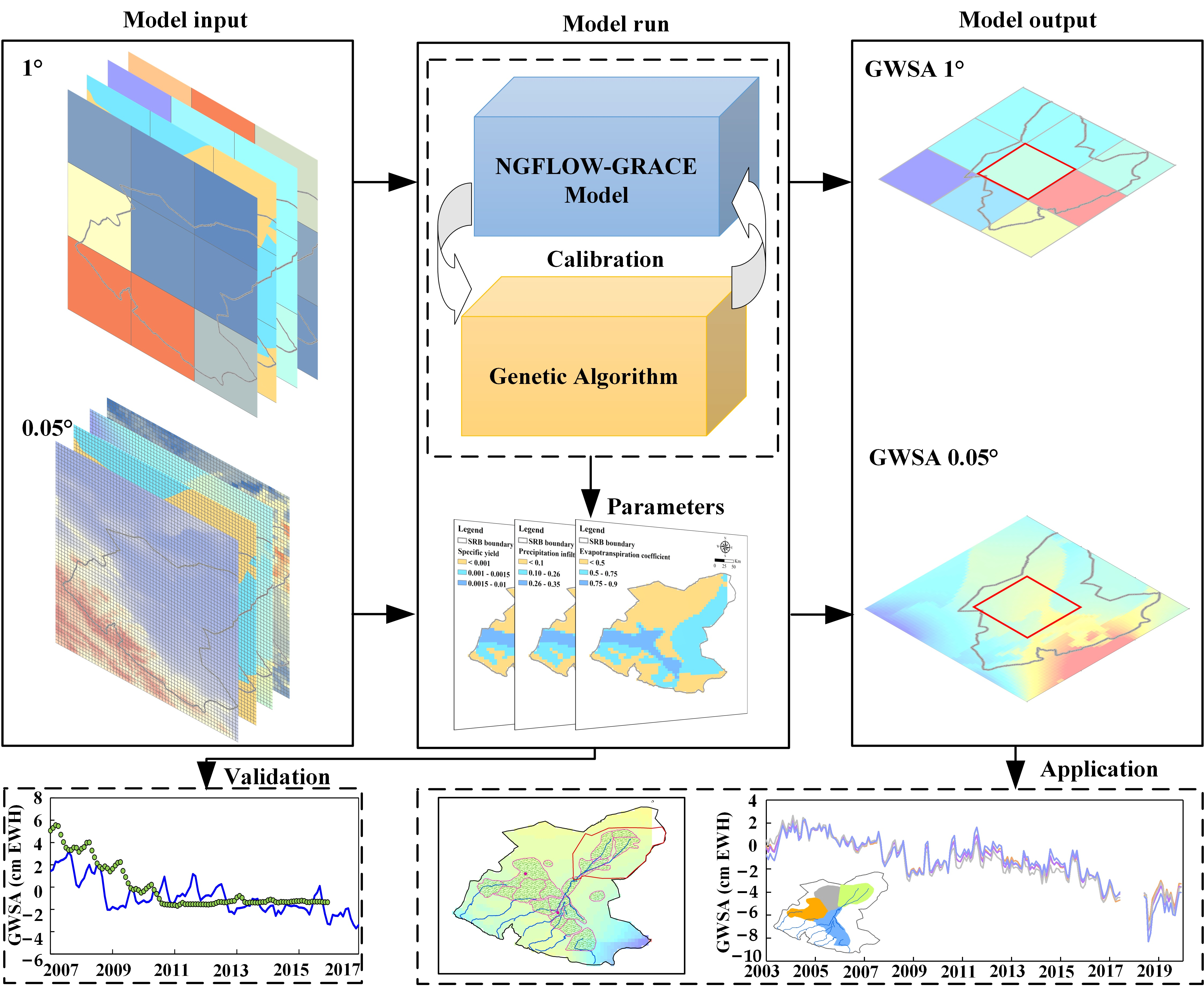
3.4. Model Development

The GRACE-derived GWSA reflects groundwater storage anomalies over the entire aquifer thickness. Thus, the transient groundwater flow model is two-dimensional, with an area ranging between 100° and 105° longitude and 36° and 41° latitude. The study area was discretized into 25 grid cells, and the grid size was set to 1°, which was consistent with the resolution of the GRACE data. The outer grids of the model are regarded as Dirichlet boundaries (cells G1-G6, G10-G11, G15-G16, G20-G25), and the GWSA in nine inner grid cells was simulated (Figure 3). The changes in the surface water were very small and were ignored in this study. Precipitation infiltration was the main recharge source. The main discharge items were evapotranspiration and groundwater exploitation. Almost 90% of the groundwater use is for agricultural irrigation; and thus, most of the irrigation water is lost through ET. Groundwater discharge can be determined by the actual evapotranspiration and the coefficient.
The parameters of the model include the transmissivity (T), comprehensive specific yield (u), precipitation infiltration coefficient (α), evapotranspiration coefficient (β), and hydraulic gradient coefficient (Ch). Based on the hydrogeological features, the study area is generalized into three zones: a highly permeable alluvial–proluvial pore aquifer (Zone P1); medium-permeability fractured aquifers hosted in magmatic, sedimentary, and metamorphic rocks (Zone P2); and a weakly permeable porous aquifer in the loess layer of the Loess Plateau (Zone P3) (Figure 3). When the parameter values in each zone are known, the parameters of each grid can be estimated using the following formula:
P G i = k = 1 3 A r e a k × P k
where P G i represents grid Gi parameter, A r e a k represents area percentage for different aquifers, and Pk represents the parameters (transmissivity, comprehensive specific yield, precipitation infiltration, and evapotranspiration coefficient) for the kth type of aquifer.

4. Results

4.1. Model Calibration and Validation

The calibration and validation periods of the model were January 2003 to June 2017 and June 2018 to December 2019, respectively. The time step was one month. Using the GRACE-derived GWSA in January 2003 as the initial condition, the time-series GRACE-derived GWSA in the outer cells of Figure 3 was used as the boundary data. Given the parameter threshold (Table S1), the genetic algorithm toolkit GeatPy [24] was used to estimate and obtain the optimal parameters (Figure S1). Figure 4 shows a comparison of the GRACE-derived and simulated GWSA in both the calibration and validation periods. Generally, the correlation coefficients of the grid cells except the G12 cell were over 0.60 (Table 2), and the RMSEs of the grid cells were within 1.00 cm equivalent water height (EWH) in the calibration period and validation period. The difference between the simulated and GRACE-derived results in grid cell G12 is large, with an RMSE of 2.38 cm EWH, probably because of the influences of boundary conditions. Overall, the simulated GWSA maintained similar patterns to the GRACE-derived results during both the calibration and validation periods.

4.2. Model Uncertainty Analysis

Model accuracy is restricted by uncertainties in climate forcing, such as precipitation, actual evapotranspiration data, and model parameters. Thus, uncertainty analysis of the model parameters, forcing data, and boundary conditions was performed. The Morris global sensitivity analysis method was used to evaluate the sensitivity of hydrogeological parameters. A total of 1000 groups of sampling parameters were generated using the Monte Carlo method. The sensitivity of the hydraulic gradient coefficient was significantly higher than that of the other parameters, and transmissivity had the smallest sensitivity (Figure S2). Six different combinations of precipitation and evapotranspiration data (TRMM-GLEAM, TRMM-MODIS, PENG-GLEAM, PENG-MODIS, ERA-ERA, and ERA-MODIS) were applied to the model with the same hydrogeological parameters. It was found that the results from the six combinations had consistent changing patterns, and the correlation coefficients between them were over 0.9 with RMSEs smaller than 0.75 cm EWH. The different forcing data had no obvious impact on the model results (Figure S3).
To study the influence of the model boundary on the simulation results, it is assumed that due to climate change, the snow water on the southern Qilian Mountains melts over time, and thus, the groundwater storage on the boundary is increased. The hydrogeological parameters, sources, and sinks remained unchanged. The GWSA in grid cells G6, G11, and G16 was increased by 10%, 30%, and 50%, respectively, to analyze its influence on the simulation results. Figure 5 shows that the RMSEs in the southern grid cells (G7, G12, G17) showed the most significant change, and the influences gradually decreased towards the northern cells. Therefore, the boundary conditions of the model have a significant impact on the model results and should be carefully evaluated.

4.3. Downscaling of GWSA Data

After model calibration and validation, nine grid cells in the middle of the study area were subdivided from 1° (Figure 6a) to 0.05° (Figure 6c). The study area was further discretized into 3600 grid cells. GRACE-derived GWSA was used as the model boundary and initial conditions, and the hydrogeological parameters were processed using Equation (10) with a spatial resolution of 0.05°. Precipitation data from PENG and actual evapotranspiration data from MODIS were used to drive the downscaling model.
The simulation period for the downscaled model was from January 2003 to December 2019 without a gap between GRACE and GRACE-FO. Figure 6d shows that the overall pattern of downscaling GWSA is similar to that of GRACE-derived GWSA (Figure 6b), which not only retains the original GWSA feature but also captures fine groundwater storage changes. It can be seen from the downscaled time-series GWSA in each grid cell (Figure 7) that the pattern is consistent with that of GRACE-derived GWSA.

4.4. Validation of Downscaling Results

Groundwater level data from field observations can be converted into GWSA data by subtracting the average groundwater level from 2007 to 2009 and multiplying by the comprehensive specific yield. It can be found from the comparison of simulated and observed results in Figure 8 that the trend of downscaled GWSA is consistent with that estimated from field observations. The changes in groundwater storage in W1, W4, W5, and W6 match well with the downscaled GWSA with correlation coefficients greater than 0.50. The negative correlation coefficients between W2 and W3 may be affected by local groundwater extraction, which was not refined and considered in the downscaled model. In general, the downscaled GWSA can capture groundwater storage variation on a small scale.

5. Discussion

5.1. Basin-Scale Groundwater Storage Anomaly Changes

The SRB governance project has been officially implemented since 2007, with the first phase of governance occurring between 2007 and 2010 and the second phase between 2011 and 2016. The simulated monthly changing trends of groundwater storage were calculated by applying linear regression during 2003–2006, 2007–2010, 2011–2016, and 2018–2019, and the spatial distribution of the groundwater storage changing trend in the SRB was obtained (Figure 9a–d). The groundwater storage changes in the SRB can be divided into six types, which are rapid decline, decline, slow decline, slow rise, rise, and rapid rise (Table 3). Groundwater storage decreased from 2003 to 2006 in most areas of the SRB (Figure 9a), accounting for 66.4% of the total area, and the area with a slow rise accounted for 27.6%, which was mainly distributed in the southern mountainous areas. Chen et al. [25] found that the areas with a depth to groundwater of over 20 m grew from 27.3% to 62.6% from 1999 to 2008, and this similar result demonstrates that groundwater in the study area was being depleted at an accelerated rate before the governance project was implemented. From 2007 to 2010, the groundwater storage generally decreased, and the areas with declining and rapidly declining GWSA accounted for 74.5% of the total area, with an increase of 45.30% compared with the period from 2003 to 2006.
During this period, the areas with declining and rapidly declining GWSA were mainly distributed in the central irrigation area and Minqin Basin, where there were higher densities of pumping wells. Depths to groundwater were deepened to over 30 m in some regions, and the cone of groundwater depletion also increased synchronously [26]. A similar conclusion was also found by Feng et al. [27] in the study area. Due to the reduction in GWS and the domination of oasis shrinkage, although oasification and desertification occurred simultaneously in the SRB from 2005 to 2010, the net reduction in the oasis area is approximately 300 km2 [28]. The rapid decline of GWS in the oasis is mainly affected by population growth, increased cultivated land area, and agricultural production [29]. From 2011 to 2016, the area with a rapidly declining GWSA decreased, but the area with declining GWSA increased. The declining trend of GWSA in the Minqin Basin improved, and areas with rapidly declining GWSA were mainly concentrated in the southern mountains. From July 2018 to December 2019, the groundwater storage in the SRB significantly recovered, and the groundwater storage in the entire region showed an increasing trend. Thus, the GWS recovery was not clearly observed in the first stage of comprehensive management of SRB because the process of aquifer recovery is long and slow [30].

5.2. Subregion-Scale Groundwater Storage Anomaly Changes

Four sub-basins, the Wuwei sub-basin (WWB), the Minqin sub-basin (MQB), the Yongchang sub-basin (YCB), and the Jinchuan sub-basin (JCB), were chosen to analyze the GWSA changes. The WWB and YCB are located upstream of the SYB, whereas the MQB and JCB are located downstream. Figure 10a shows the monthly GWSA data from 2003 to 2019. From 2003 to 2010, the GWSA in the four subregions and that in the entire study area were effectively the same. After 2010, GWSA showed some differences in each subregion; the GWSA in WWB and MQB was significantly higher than that in other basins in both peak and valley values. In general, the declining trend of GWSA in the four sub-basins was similar to that in the entire area, which was the sharp increase in GWSA in 2003, followed by a continuous declining trend from 2004 to 2008; from 2009 to 2011, there was another slowly increasing trend, followed by another decline. Since June 2018, GWSA has gradually recovered. Figure 10b shows the annual mean GWSA between 2003 and 2016 and the anomalies in precipitation and AET relative to the mean between 2004 and 2009, indicating an overall downward trend in GWSA. The annual decline rates of GWSA were 0.26 cm/year, 0.32 cm/year, 0.22 cm/year, 0.22 cm/year, and 0.28 cm/year in SRB, JCB, MQB, WWB, and YCB, respectively. The decline rate in the SRB found in this study was similar to the results obtained by Wang et al. [31] in the Hexi Corridor and close to the average declining rate of 0.29 cm/year calculated by Liu et al. [32]. By analyzing the relationship between meteorological factors and GWSA, it was found that in years when the GWSA decreased rapidly, such as in 2009 and 2016, the AET was greater than the precipitation in the previous year. Due to drought, decreased upstream inflows and increased extraction of groundwater ultimately lead to a decline in groundwater storage, which is consistent with the results of Liu et al. [32]. Figure 10c shows the interannual seasonal variations in GWSA, precipitation, and AET. GWSA showed similar trends to seasonal changes. The GWSA declined rapidly from March to May, which may be because, with less precipitation during this period, crop cultivation and irrigation in spring required a larger amount of water. From June to August, precipitation increased significantly in the summer, and groundwater recovered. In August, precipitation peaked. From September to October, the decline in GWSA became severe because of irrigation in the autumn. From November to February of the following year, groundwater storage gradually recovered.
It can be seen that the GWSA in the WWB and MQB had a large change range. Agriculture in these two areas was relatively developed, and the groundwater level fluctuated greatly during the irrigation period. Precipitation in mountainous areas mainly enters the WWB through rivers flowing out of the mountains, and groundwater finally flows into the MQB in the form of lateral runoff. Increased water resource consumption in the middle reaches of the WWB affects the change in GWSA in the MQB [33]. Industrial water consumption in the JCB and YCB was large, but the water consumption was relatively stable, and the fluctuation in the groundwater level during the year was relatively small.

5.3. Comparison of GWS Changes from Downscaled and Field Observations

The monthly GWS changes from the downscaled model and field observations in the midstream WWB and downstream MQB from 2007 to 2016 are compared. The monthly GWS changes can be calculated from Equation (9). Figure 11 shows that the GWS change trend and magnitude were approximately similar between downscaled and field observations before 2012. GWS change fluctuations from field observations in the midstream of the WWB subregion were larger than those in the downstream region of MQB, which may be attributed to massive groundwater extraction for agricultural irrigation and quick lateral recharge from piedmont precipitation in the midstream WWB. After 2012, the magnitude of GWS changes from field observations became stable, indicating that groundwater level changes tend to stabilize. However, downscaled GWS changes were more sensitive than those from field observations, which may be attributed to the change in aquifer specific yield with groundwater extraction, where a constant specific yield was used in this study to convert groundwater level to groundwater storage. The specific variation mechanism of aquifer parameters with groundwater extraction still requires professional in-depth study.
In addition, it was also observed that there was a 4-month time lag of GWS changes between the downscaled and field observations, which was even more significant between 2007 and 2012. However, the lag time reported by Wang et al. [31] was 3 months in this study area. A similar time lag was also reported in other study areas, such as 3 months in southwestern Iran [34] and 2 months in the Central Valley of California [35]. Time lags in wetter climates have not been observed in some studies, such as in the Loess Plateau of northern China [36] and the Indus Basin [37]. The differences in time lags are various [31] for many reasons, including (1) meteorological conditions in arid environments (for example, the insufficient precipitation and thick vadose zone hinder the timely recharge of groundwater aquifers); (2) the GRACE-derived GWSA from different hydrological models with different types of data input, such as the GLDAS data used in this study; (3) the spatial representation of the field observation data also affecting the time lag (for example, most of the monitoring wells were distributed in the oases in this study area, which had different groundwater dynamic types from those distributed in the surrounding desert; moreover, the GWS estimated with a limited number of monitoring wells cannot adequately represent the overall GWS changes).

5.4. Limitations and Perspectives

GRACE data are mainly used to represent changes in regional terrestrial water storage. GWS changes can only be obtained by subtracting components such as soil water storage and snow water equivalent changes. In this study, the components were derived from the GLDAS hydrological model, which makes it difficult to monitor short-term activities such as mining and artificial water diversion. Therefore, the estimation of water storage changes from the GLDAS hydrological model is uncertain on a short time scale, but it reliably reflects the long-term trend.
Limited by the data collected from the study area, only precipitation and actual evapotranspiration were considered as the source and sink terms of the groundwater storage model, but surface water infiltration and local groundwater exploitation are also part of the source and sink terms in the study area and were not fully considered in this model. The area of the groundwater storage model is relatively large; thus, heterogeneity of this model parameter occurred, which would affect the model accuracy. Although the results are satisfactory, if more detailed data are provided for subsequent research, such as sufficient groundwater level data and detailed hydrogeological parameters, the model can be further improved.
In this study, only GWSA data were used to develop a groundwater storage model, and the integration of GRACE-derived GWSA data and field observation data will be considered to constrain the model parameters in future studies. In addition, this study only considered the spatial downscaling of GRACE data; if driving data with a higher temporal resolution can be collected in subsequent studies, the temporal resolution of GRACE can be downscaled from the monthly scale to the daily scale or even smaller resolutions. Finally, this study did not interpolate GRACE and GRACE-FO satellite data during the gap period. These are the directions for our further in-depth research in the future.

6. Conclusions

In this study, to overcome the limitation of the coarse spatial resolution of GRACE data, a groundwater storage model was constructed in the SRB using GRACE-derived GWSA data as the independent variable to downscale groundwater storage changes. A genetic algorithm was used to optimize the parameters, and the calibrated model was applied to spatially downscale the GWSA data from 1° to 0.05°. The reliability of the downscaled data was verified through observations and comparisons with those of other studies. The main conclusions are as follows:
(1)
The changes in the simulated groundwater storage anomalies fit well with the observed values, and the correlation coefficients between the simulated and observed values were generally over 0.6 in both the calibration and validation periods. The uncertainty analysis of the model showed that the boundary conditions had a greater impact on the model results, whereas the precipitation and evapotranspiration data from different sources had no obvious effect on the results. The sensitivity of the hydraulic gradient coefficient was significantly higher than that of the other parameters.
(2)
The downscaled GWSA maintains a spatial distribution and time-series changing patterns similar to those of the GRACE-derived GWSA, as well as capturing more fine groundwater storage features. The changing patterns of the downscaled GWSA were consistent with those from the observation well data.
(3)
The GWS generally showed a downward trend from 2003 to 2019. In the initial stage of groundwater governance implementation, the overall GWS decreased and only increased slightly from 2009 to 2011. After 2012, the downward trend in GWS did not slow down significantly. Since June 2018, the areas of GWS increase were mainly distributed in the southern piedmont area.
(4)
The annual decline rates of GWSA from 2003 to 2016 were 0.26 cm/year, 0.32 cm/year, 0.22 cm/year, 0.22 cm/year, and 0.28 cm/year in SRB, JCB, MQB, WWB, and YCB, respectively. The GWS changes in the MQB are mainly affected by the exploitation and utilization of water resources in the WWB, and the change trend of the GWS between the MQB and WWB is highly consistent. In addition, there was a four-month time lag between the field observations and downscaled GWSA changes.
Overall, this study provides methodological guidance for the application of GRACE data in the assessment of groundwater storage changes in small-scale areas.

Supplementary Materials

The following supporting information can be downloaded at: https://www.mdpi.com/article/10.3390/rs14194719/s1, Table S1: Parameter thresholds of the model. Figure S1: Spatial distribution of (a) comprehensive specific yield, (b) precipitation infiltration coefficients, and (c) evapotranspiration coefficient in the study area. Figure S2: Sensitivities of model parameters. Figure S3: Effects of different forcing data combinations on simulated groundwater storage changes.

Author Contributions

J.S.: writing—original draft, writing—review and editing; L.H.: conceptualization, methodology, writing—review and editing; X.L.: data collection and analysis, discussion, writing—review and editing; K.S.: writing—review and editing. All authors have read and agreed to the published version of the manuscript.

Funding

This research was funded by the National Natural Science Foundation of China, grant numbers 41877173 and U2167211.

Acknowledgments

We appreciate the free access to the GRACE mascons solutions and GLDAS, TRMM, ERA5, GLEAM, MODIS, and PENG meteorological and hydrological datasets. GRACE mascons solutions: ftp://podaac-ftp.jpl.nasa.gov/allData/tellus/L3/land mass/RL06 (accessed on 11 March 2022); GLDAS: http://disc.gsfc.nasa.gov/hydrology/data-holdings (accessed on 11 March 2022); GLEAM: http://www.gleam.eu (accessed on 16 March 2022); MODIS: https://doi.org/10.5067/MODIS/MCD12Q1.006 (accessed on 16 March 2022); TRMM: https://gpm.nasa.gov/category/mission-affiliation/trmm (accessed on 21 March 2022); ERA5: https://cds.climate.copernicus.eu/cdsapp#!/home (accessed on 23 March 2022); PENG: http://poles.tpdc.ac.cn/zh-hans/data/faae7605-a0f2-4d18-b28f-5cee413766a2/ (accessed on 02 April 2022).

Conflicts of Interest

The authors declare no conflict of interest.

References

  1. Taylor, R.G.; Scanlon, B.; Döll, P.; Rodell, M.; Van Beek, R.; Wada, Y.; Longuevergne, L.; Leblanc, M.; Famiglietti, J.S.; Edmunds, M.; et al. Ground water and climate change. Nat. Clim. Chang. 2013, 3, 322–329. [Google Scholar] [CrossRef]
  2. Jasechko, S.; Perrone, D.; Befus, K.M.; Bayani Cardenas, M.; Ferguson, G.; Gleeson, T.; Luijendijk, E.; McDonnell, J.J.; Taylor, R.G.; Wada, Y.; et al. Global aquifers dominated by fossil groundwaters but wells vulnerable to modern contamination. Nat. Geosci. 2017, 10, 425–429. [Google Scholar] [CrossRef]
  3. Dalin, C.; Wada, Y.; Kastner, T.; Puma, M.J. Groundwater depletion embedded in international food trade. Nature 2017, 543, 700–704. [Google Scholar] [CrossRef] [PubMed]
  4. Ahamed, A.; Knight, R.; Alam, S.; Pauloo, R.; Melton, F. Assessing the utility of remote sensing data to accurately estimate changes in groundwater storage. Sci. Total Environ. 2021, 807, 150635. [Google Scholar] [CrossRef]
  5. Rodell, M.; Velicogna, I.; Famiglietti, J.S. Satellite-based estimates of groundwater depletion in India. Nature 2009, 460, 999–1002. [Google Scholar] [CrossRef]
  6. Tapley, B.; Bettadpur, S.; Ries, J.; Thompson, P.; Watkins, M. GRACE measurements of mass variability in the Earth system. Science 2004, 305, 503–505. [Google Scholar] [CrossRef]
  7. Li, B.; Rodell, M.; Kumar, S.; Beaudoing, H.K.; Getirana, A.; Zaitchik, B.F.; de Goncalves, L.G.; Cossetin, C.; Bhanja, S.; Mukherjee, A.; et al. Global GRACE data assimilation for groundwater and drought monitoring: Advances and challenges. Water Resour. Res. 2019, 55, 7564–7586. [Google Scholar] [CrossRef]
  8. Feng, W.; Zhong, M.; Lemoine, J.M.; Biancale, R.; Hsu, H.T.; Xia, J. Evaluation of groundwater depletion in North China using the Gravity Recovery and Climate Experiment (GRACE) data and ground-based measurements. Water Resour. Res. 2013, 49, 2110–2118. [Google Scholar] [CrossRef]
  9. Swenson, S.; Yeh, P.J.F.; Wahr, J.; Famiglietti, J. A comparison of terrestrial water storage variations from GRACE with in situ measurements from Illinois. Geophys. Res. Lett. 2006, 33, 627–642. [Google Scholar] [CrossRef]
  10. Famiglietti, J.S.; Lo, M.; Ho, S.L.; Bethune, J.; Anderson, K.J.; Syed, T.H.; Rodell, M. Satellites measure recent rates of groundwater depletion in California’s Central Valley. Geophys. Res. Lett. 2011, 38, L16401. [Google Scholar] [CrossRef] [Green Version]
  11. Wilby, R.L.; Wigley, T.M.L.; Conway, D.; Jones, P.D.; Hewitson, B.C.; Main, J.; Wilks, D.S. Statistical downscaling of general circulation model output: A comparison of methods. Water Resour. Res. 1998, 34, 2995–3008. [Google Scholar] [CrossRef]
  12. Vishwakarma, B.D.; Zhang, J.; Sneeuw, N. Downscaling GRACE total water storage change using partial least squares regression. Sci. Data. 2021, 8, 95. [Google Scholar] [CrossRef] [PubMed]
  13. Ning, S.W.; Ishidaira, H.; Wang, J. Statistical downscaling of GRACE-derived terrestrial water storage using satellite and GLDAS products. J. Jpn. Soc. Civ. Eng. 2014, 70, 133–138. [Google Scholar] [CrossRef]
  14. Yin, W.; Hu, L.; Zhang, M.; Wang, J.; Han, S.C. Statistical downscaling of GRACE-derived groundwater storage using ET data in the North China plain. J. Geophys. Res. Atmos. 2018, 123, 5973–5987. [Google Scholar] [CrossRef]
  15. Miro, M.E.; Famiglietti, J.S. Downscaling GRACE remote sensing datasets to high-resolution groundwater storage change maps of California’s Central Valley. Remote Sens. 2018, 10, 143. [Google Scholar] [CrossRef]
  16. Chen, L.; He, Q.; Liu, K.; Li, J.; Jing, C. Downscaling of GRACE-derived groundwater storage based on the random forest model. Remote Sens. 2019, 11, 2979. [Google Scholar] [CrossRef]
  17. Seyoum, W.M.; Kwon, D.; Milewski, A.M. Downscaling GRACE TWSA data into high-resolution groundwater level anomaly using machine learning-based models in a glacial aquifer system. Remote Sens. 2019, 11, 824. [Google Scholar] [CrossRef]
  18. Zaitchik, B.F.; Rodell, M.; Reichle, R.H. Assimilation of GRACE terrestrial water storage data into a land surface model: Results for the Mississippi River Basin. J. Hydrometeorol. 2008, 9, 535–548. [Google Scholar] [CrossRef]
  19. Zhong, D.; Wang, S.; Li, J. A self-calibration variance-component model for spatial downscaling of GRACE observations using land surface model outputs. Water Resour. Res. 2021, 57, e2020WR028944. [Google Scholar] [CrossRef]
  20. Hu, L.; Jiao, J.J. Calibration of a large-scale groundwater flow model using GRACE data: A case study in the Qaidam Basin, China. Hydrogeol. J. 2015, 23, 1305–1317. [Google Scholar] [CrossRef]
  21. Sun, A.Y.; Green, R.; Swenson, S.; Rodell, M. Toward calibration of regional groundwater models using GRACE data. J. Hydrol. 2012, 422, 1–9. [Google Scholar] [CrossRef]
  22. Hu, L.T.; Wang, Z.J.; Tian, W.; Zhao, J.S. Coupled surface water-groundwater model and its application in the arid Shiyang River basin, China. Hydrol. Process. Int. J. 2009, 23, 2033–2044. [Google Scholar] [CrossRef]
  23. Long, D.; Yang, Y.; Wada, Y.; Hong, Y.; Liang, W.; Chen, Y.; Yong, B.; Hou, A.; Wei, J.; Chen, L. Deriving scaling factors using a global hydrological model to restore GRACE total water storage changes for China’s Yangtze River Basin. Remote Sens. Environ. 2015, 168, 177–193. [Google Scholar] [CrossRef]
  24. Whitley, D. A genetic algorithm tutorial. Stat. Comput. 1994, 4, 65–85. [Google Scholar] [CrossRef]
  25. Chen, L.; Feng, Q. Geostatistical analysis of temporal and spatial variations in groundwater levels and quality in the Minqin oasis, Northwest China. Environ. Earth Sci. 2013, 70, 1367–1378. [Google Scholar] [CrossRef]
  26. Hao, Y.; Xie, Y.; Ma, J.; Zhang, W. The critical role of local policy effects in arid watershed groundwater resources sustainability: A case study in the Minqin oasis, China. Sci. Total Environ. 2017, 601, 1084–1096. [Google Scholar] [CrossRef]
  27. Feng, S.; Kang, S.; Huo, Z.; Chen, S.; Mao, X. Neural networks to simulate regional ground water levels affected by human activities. Groundwater 2018, 46, 80–90. [Google Scholar] [CrossRef]
  28. Xie, Y.; Bie, Q.; Lu, H.; He, L. Spatio-temporal changes of oases in the Hexi Corridor over the past 30 years. Sustainability 2018, 10, 4489. [Google Scholar] [CrossRef]
  29. Xiao, D.; Li, X.; Song, D.; Yang, G. Temporal and spatial dynamical simulation of groundwater characteristics in Minqin Oasis. Sci. China Ser. D-Earth Sci. 2007, 50, 261–273. [Google Scholar] [CrossRef]
  30. Aeschbach-Hertig, W.; Gleeson, T. Regional strategies for the accelerating global problem of groundwater depletion. Nat. Geosci. 2012, 5, 853–861. [Google Scholar] [CrossRef]
  31. Wang, S.; Liu, H.; Yu, Y.; Zhao, W.; Yang, Q.; Liu, J. Evaluation of groundwater sustainability in the arid Hexi Corridor of Northwestern China, using GRACE, GLDAS and measured groundwater data products. Sci. Total Environ. 2020, 705, 135829. [Google Scholar] [CrossRef] [PubMed]
  32. Liu, X.; Hu, L.; Sun, K.; Yang, Z.; Sun, J.; Yin, W. Improved understanding of groundwater storage changes under the influence of river basin governance in northwestern China using GRACE data. Remote Sens. 2021, 13, 2672. [Google Scholar] [CrossRef]
  33. Aarnoudse, E.; Bluemling, B.; Qu, W.; Herzfeld, T. Groundwater regulation in case of overdraft: National groundwater policy implementation in north-west China. Int. J. Water Resour. D 2019, 35, 264–282. [Google Scholar] [CrossRef]
  34. Abou Zaki, N.; Torabi Haghighi, A.; Rossi, P.M.; Tourian, M.J.; Klove, B. Monitoring groundwater storage depletion using gravity recovery and climate experiment (GRACE) data in the semi-arid catchments. Hydrol. Earth Syst. Sci. 2018, 1–21. [Google Scholar] [CrossRef]
  35. Thomas, B.F.; Famiglietti, J.S.; Landerer, F.W.; Wiese, D.N.; Molotch, N.P.; Argus, D.F. GRACE groundwater drought index: Evaluation of California Central Valley groundwater drought. Remote Sens. Environ. 2017, 198, 384–392. [Google Scholar] [CrossRef]
  36. Xie, X.; Xu, C.; Wen, Y.; Li, W. Monitoring groundwater storage changes in the Loess Plateau using GRACE satellite gravity data, hydrological models and coal mining data. Remote Sens. 2018, 10, 605. [Google Scholar] [CrossRef]
  37. Iqbal, N.; Hossain, F.; Lee, H.; Akhter, G. Integrated groundwater resource management in Indus Basin using satellite gravimetry and physical modeling tools. Environ. Monit. Assess. 2017, 189, 128. [Google Scholar] [CrossRef]
Figure 1. Map of the study area.
Remotesensing 14 04719 g001
Figure 2. Comparison of different precipitation and actual evapotranspiration data sources in SRB from 2003 to 2019: (a) monthly precipitation; (b) actual evapotranspiration.
Remotesensing 14 04719 g002
Figure 3. Distribution of parameter zones and Dirichlet boundaries in the study area.
Remotesensing 14 04719 g003
Figure 4. Simulated GWSA from January 2003 to December 2019.
Remotesensing 14 04719 g004
Figure 5. Influence of changing model boundary conditions on model simulation results.
Remotesensing 14 04719 g005
Figure 6. Comparison of groundwater storage changes before and after the downscaling in December 2019. (a,c) The 1° and 0.05° mesh grid blocks, respectively; (b,d) the spatial distribution of GWSA before and after downscaling.
Remotesensing 14 04719 g006
Figure 7. Time-series trend of downscaling results from 2003 to 2019. The red band represents the changes in GWSA within all 0.05° grids under the 1° grid, and the blue scatters represent GRACE-derived GWSA in the 1° grid.
Remotesensing 14 04719 g007
Figure 8. Comparison of time-series groundwater storage changes from the model and field observation.
Remotesensing 14 04719 g008
Figure 9. Spatial distribution of groundwater storage anomaly change rate in the SRB in four phases: (a) 2003–2006, (b) 2007–2010, (c) 2011–2016, and (d) July 2018 to December 2019.
Remotesensing 14 04719 g009
Figure 10. Changes of groundwater storage anomalies in subregions from 2003 to 2019: (a) represents the monthly GWSA changes of different subregions, (b) represents the annual mean variation of the groundwater storage, precipitation (P) and actual evapotranspiration (AET) anomalies, (c) represents the interannual seasonal variations of the GWSA, precipitation and actual evapotranspiration.
Remotesensing 14 04719 g010
Figure 11. Comparison of GWS changes from downscaled and field observations in (a) WWB and (b) MQB. GWL-evaluated and GWL-evaluated-4 represent GWS changes of field observations at the current month and 4-month time lag, respectively.
Remotesensing 14 04719 g011
Table 1. Data sources used in this study.
Data ItemSourceSpatial ResolutionTime ResolutionTime Span (Year)
TWSGRACE0.5°Monthly2003–2019
SM, SWEGLDAS V2.1Monthly2003–2019
PrecipitationTRMM 3B430.25°Monthly2003–2019
ERA50.25°Monthly2003–2019
PENG0.05°Monthly2003–2019
AETGLEAM v3.50.25°Monthly2003–2019
MODIS0.05°Monthly2003–2019
ERA50.25°Monthly2003–2019
GWLIn situ observation-Daily2007–2018
Table 2. Coefficient and RMSE for each cell in the calibration and validation periods.
Cell IDCalibration PeriodValidation Period
CCRMSECCRMSE
G70.890.770.521.42
G80.911.570.641.08
G90.880.740.920.98
G120.651.550.442.38
G130.921.310.590.99
G140.890.800.900.83
G170.601.260.851.61
G180.921.040.810.69
G190.941.010.840.75
Table 3. Area percentage of six types of groundwater storage changes in the SRB from 2003 to 2019.
Time PeriodRapid DeclineDeclineSlow DeclineSlow RiseRiseRapid Rise
2003–20061.3%27.9%37.2%27.6%6.0%0.0%
2007–201024.0%50.5%25.5%0.0%0.0%0.0%
2011–2017.614.2%72.7%13.1%0.0%0.0%0.0%
2018.6–2019.120.0%0.0%0.0%5.1%23.6%71.3%
Publisher’s Note: MDPI stays neutral with regard to jurisdictional claims in published maps and institutional affiliations.

