Article

Study and Prediction of Surface Deformation Characteristics of Different Vegetation Types in the Permafrost Zone of Linzhi, Tibet

College of Forestry, Beijing Forestry University, Beijing 100083, China
*
Author to whom correspondence should be addressed.
Remote Sens. 2022, 14(18), 4684; https://doi.org/10.3390/rs14184684
Submission received: 23 July 2022 / Revised: 9 September 2022 / Accepted: 13 September 2022 / Published: 19 September 2022

Abstract

:
Permafrost and alpine vegetation are widely distributed in Tibet, which is a sensitive area for global climate change. In this study, we inverted the surface deformation from 22 May 2018 to 9 October 2021 in a rectangular area within the city of Linzhi, Tibet, using the Sentinel1-A data and two time-series interferometric system aperture radar (InSAR) techniques. Then, the significant features of surface deformation were analyzed separately according to different vegetation types. Finally, multiple machine learning methods were used to predict future surface deformation, and the results were compared to obtain the model with the highest prediction accuracy. This study aims to provide a scientific reference and decision basis for global ecological security and sustainable development. The results showed that the surface deformation rate in the study area was basically between ±10 mm/a, and the cumulative surface deformation was basically between ±35 mm. The surface deformation of grassland, meadow, coniferous forest, and alpine vegetation were all significantly correlated with NDVI, and the effect of alpine vegetation, coniferous forest, and grassland on permafrost was stronger than that of the meadow. The prediction accuracy of the Holt–Winters model was higher than that of Holt′s model and the ARIMA model; it was expected that the ground surface would keep rising in the next two months, and the ground surface deformation of alpine vegetation and the coniferous forest was relatively small. The above studies indicated that the surface deformation in the Tibetan permafrost region was relatively stable under the conditions of alpine vegetation and coniferous forest. Future-related ecological construction needs to pay more attention to permafrost areas under grassland and meadow conditions, which are prone to surface deformation and affect the stability of ecosystems.

Graphical Abstract

1. Introduction

With global warming, the influence of climate change on the future global ecological environment and the mechanism of the responses of ecosystems to climate change have been extensively raised and studied [1,2,3,4,5]. Tibet has a large area of high-altitude permafrost and is one of the plateau ecosystems with the highest sensitivity to global climate change [6,7,8]. The type of permafrost in northwest Tibet is dominated by perennial permafrost, while southeast Tibet is influenced by the warm and humid flow of the Indian Ocean and dominated by seasonal permafrost, i.e., the freezing of soil has seasonal changes, freezing in winter and melting in summer [9]. The freezing and thawing of permafrost significantly affect the hydrology, climate, and ecosystems of the regions in which it is located, by participating in the global cycle of energy and water. Over recent years, under climate change impact, not only has the perennial permafrost begun to degrade into seasonal permafrost extensively in Tibetan areas, but the thickness of the active layer of the existing seasonal permafrost is also increasing substantially, along with the problems of increasing the mean ground temperature of the permafrost and the advancement of the thawing date [6,10,11]. The current series of changes in the permafrost can disrupt these cyclic processes to some extent, causing soil moisture loss, land desertification, and reduced vegetation cover [12,13], thus causing far-reaching effects on the hydrological and climatic systems, and making the ecological security of alpine regions challenging.
Vegetation is not only an important medium in the global material and energy cycle but also the most intuitive indicator of global climate change, especially as the vegetation on permafrost is vulnerable to climate change. The existence and degradation of permafrost have a significant impact on the composition and structure of vegetation, and the stability of ecosystems in alpine regions [14,15]. On the other hand, different vegetation types will have corresponding feedback on the freezing and melting of permafrost, which in turn will counteract the formation and development of permafrost [16,17]. Permafrost and vegetation can slow or accelerate climate change by influencing the exchange of energy and water between the surface and the atmosphere, which in turn regulates the regional climate. Studies have shown that ecosystems located at high latitudes or high altitudes have a higher sensitivity to climate change [18,19,20]. Tibet, as a region with both a highland environment and permafrost environment, will respond more rapidly to global climate change. For example, Zhang et al. [21] found that the area of alpine wetlands in the Tibetan region decreased by about 23.35% from 1991 to 2020, the temperature was one of the main drivers of wetland changes, and the correlation between the wetland area and the rising season temperature was the largest. Liu et al. [22] explored the temporal changes in vegetation phenology on the Tibetan Plateau from 1982–2015 and found that there was an extended growing season length (GSL) in the northeast, revealing that temperature was one of the main factors determining the delayed end of the growing season (EOS). Therefore, the analysis of surface deformation under different vegetation cover types in the permafrost zone of Tibet is of great importance to research in the field of global climate.
In recent years, remote sensing has become an important tool to reveal the response and feedback mechanisms of ecosystems to global climate change because of its wide coverage, spatial continuity, and long time series. Interferometric system aperture radar (InSAR) technology, which has been rapidly developed in recent decades, is an active microwave remote sensing technology with features such as all-weather, high accuracy, and high resolution, and it has a high potential for application in conducting earth observation over large areas [23], which can accurately monitor small deformations on the surface with centimeter-level or even millimeter-level accuracy [24,25]. InSAR provides a very effective solution for monitoring small surface deformation caused by the freezing and thawing of permafrost. Later developed time-series InSAR techniques are represented by Persistent Scattering InSAR (PS-InSAR), which can remove most of the atmospheric factors; and Small Baseline Subset InSAR (SBAS-InSAR), which can remove most of the decorrelation and elevation error effects. These technologies further improve the detection accuracy due to the spatial–temporal irrelevance, vegetation occlusion, etc. [26,27,28]. Presently, time-series InSAR technology has been well applied in the field of high-accuracy monitoring and analysis of surface deformation in permafrost areas. Chen et al. [29] observed the surface deformation in the permafrost area of the Qinghai-Tibet Plateau from 2014 to 2019 based on the time-series InSAR technique, and the results showed that the seasonal deformation was as high as 80 mm and the average settlement value was about 10 mm. Zhao et al. [30] constructed a deformation model that took into account factors such as climate and tectonic activity and combined it with SBAS-InSAR to monitor and revise surface deformation in the southern permafrost zone of the Tibetan Plateau. Rouyet et al. [31] used InSAR technology to monitor the permafrost area of the Svalbard Islands, which was also at high latitude and altitude, and found that surface subsidence and uplift could match the thawing and freezing dates of the permafrost, and analyzed the correspondence between surface deformation and seasonal changes in surface temperature. However, most of the current studies only focus on the topics of surface deformation, active layer thickness, and thawing dates in the permafrost area, while the monitoring results have rarely been applied to reveal the surface deformation characteristics under different vegetation conditions. Given this, this paper took the permafrost area under different vegetation cover types in the Tibetan region as the research object, combined the time-series InSAR technique and a machine learning algorithm based on the Sentinel1-A data, established a regional-scale permafrost deformation monitoring and prediction method system, analyzed the relationship between surface deformation and vegetation cover types, and quantified the influence of vegetation conditions and permafrost freeze-thaw in the Tibetan region. The research results are expected to provide an important scientific basis and technical reference for ecological protection and construction in alpine regions.

2. Materials and Methods
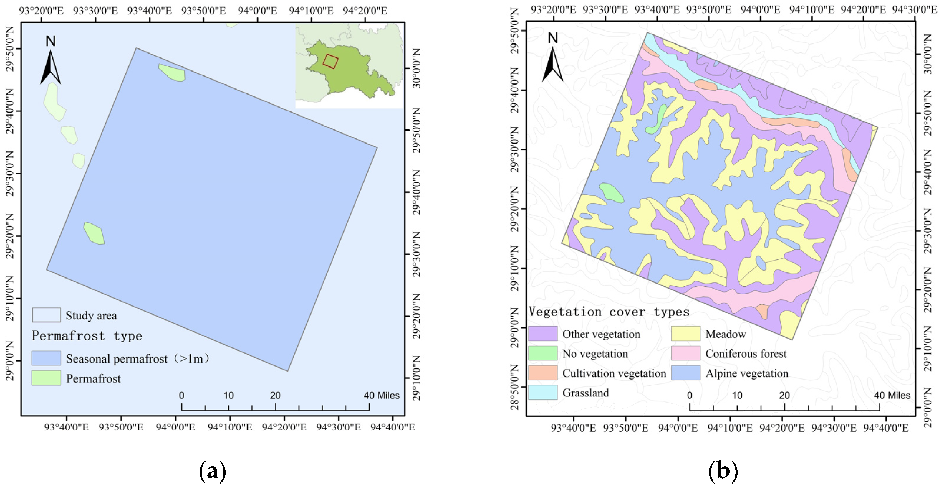
2.1. Study Area

Located in Linzhi City, Tibet, Sedgera Mountain is a typical mountain system in southeastern Tibet, located at the intersection of the Himalayan tectonic belt, the eastern end of the Nian Tanggula tectonic belt, and the tectonic belt of the Hengduan Mountains, with intense tectonic movements and active surface deformation; in addition, the Sedgera Mountain has unique climatic conditions belonging to a relatively typical subalpine temperate semi-humid climate, and under the influence of the southwest monsoon, the vegetation in the region grows luxuriantly and of many types. Therefore, in this paper, a rectangular area was selected as the study area to the south of Sedgera Mountain in Linzhi City, as shown in Figure 1. The study area is located between 29°11′ and 29°90′N latitude and 93°56′ and 94°54′E longitude, with an area of about 5796.7 km². It is a typical seasonal permafrost area, with 99% of the whole area being seasonal permafrost and 1% being perennial permafrost. The vegetation coverage is very high, and the vegetation-free area only accounts for 0.2%. The vegetation types include alpine vegetation, arable vegetation, coniferous forest, and grassland and meadow, of which alpine vegetation and meadow are the main categories.

2.2. Data Sources

In this paper, a total of 20 views of the Sentinel1-A TOPSAR data from 22 May 2018 to 9 October 2021 (https://search.asf.alaska.edu/, accessed on 14 April 2022) were used as the data source, with a spatial resolution of 5 m × 20 m, image acquisition by downlink, interferometric wide swath (IW) imaging mode, and a polarization mode of VV. Meanwhile, the POD Precise Orbit Ephemerides high-precision orbital data (https://qc.sentinel1.eo.esa.int/, accessed on 14 April 2022) with a positioning accuracy of >5 cm and 12.5 m resolution DEM data (https://qc.sentinel1.eo.esa.int/, accessed on 14 April 2022) were used as auxiliary data to further improve the accuracy and reliability of the results. In addition, NDVI data of the study area were obtained from the Landsat8 dataset of the Google Earth Engine platform (https://developers.google.cn/earth-engine, accessed on 14 April 2022), permafrost type distribution data were extracted from the China permafrost distribution map [32], and the vegetation type was taken from the 1:1,000,000 scale vegetation distribution map of China (http://westdc.westgis.ac.cn, accessed on 14 April 2022).

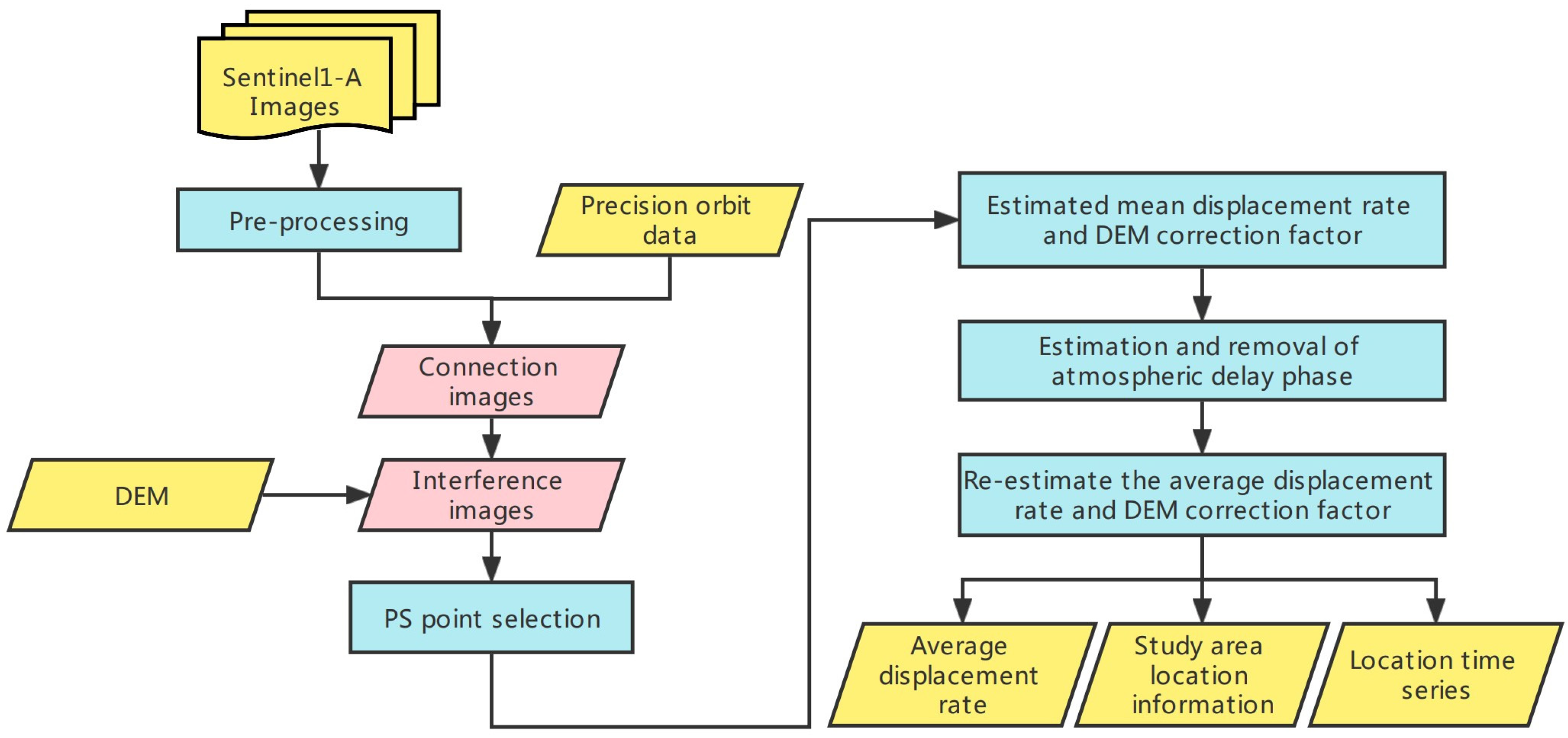
2.3. Principle of PS-InSAR

The principle of the PS-InSAR technique is to select one image among all the images as the main image by considering factors such as temporal and spatial baseline distribution, then perform differential interference processing on the images to extract PS candidate points, and finally obtain the average deformation rate and cumulative deformation value of each PS control point in the research region [33]. The interference phase composition Φ p s of every PS point is shown in Equation (1) [34]:
Φ p s = Φ f l a + Φ t o p + Φ d e f + Φ a t m + Φ n o i
where Φ f l a is the phase component caused by the flat earth effect, Φ t o p is the phase component caused by the ground elevation, Φ d e f is the phase component caused by the surface deformation, Φ a t m is the phase component caused by the atmospheric delay effect, and Φ n o i is the phase component caused by noise. The expressions of the flat earth phase Φ f l a , topographic phase Φ t o p , and the deformation phase Φ d e f are as follows:
Φ f l a = 4 Π B c o s θ α λ R t a n θ Δ R
Φ t o p = 4 Π B c o s θ α λ R s i n θ Δ h
Φ d e f = 4 Π B λ Δ d
The differential interference phase Φ d i f f of the PS point can be expressed as:
Φ d i f f = Φ f l a _ e r r o r + Φ t o p _ e r r o r + Φ d e f + Φ a t m + Φ n o i
where Φ d i f f is the differential phase after removing the flat-ground phase component as well as the topographic phase, Φ f l a _ e r r o r is the residual error when removing the flat-ground phase, and Φ t o p _ e r r o r is the residual error when removing the topographic phase, whose expressions can be expressed as:
Φ t o p _ e r r o r = 4 Π B c o s θ α λ R s i n θ Δ h e r r o r
Φ d e f = 4 Π λ   Δ d
Φ d i f f = 4 Π B c o s θ α λ R s i n θ Δ h e r r o r + 4 Π λ   Δ d + Φ r e s
Φ r e s = Φ f l a _ e r r o r + Φ a t m + Φ n o i
where 4 Π B c o s θ α λ R s i n θ Δ h e r r o r is the topographic error, 4 Π λ   Δ d is the deformation phase, and Φ r e s is the residual error.
The processing flow of PS-InSAR is shown in Figure 2.

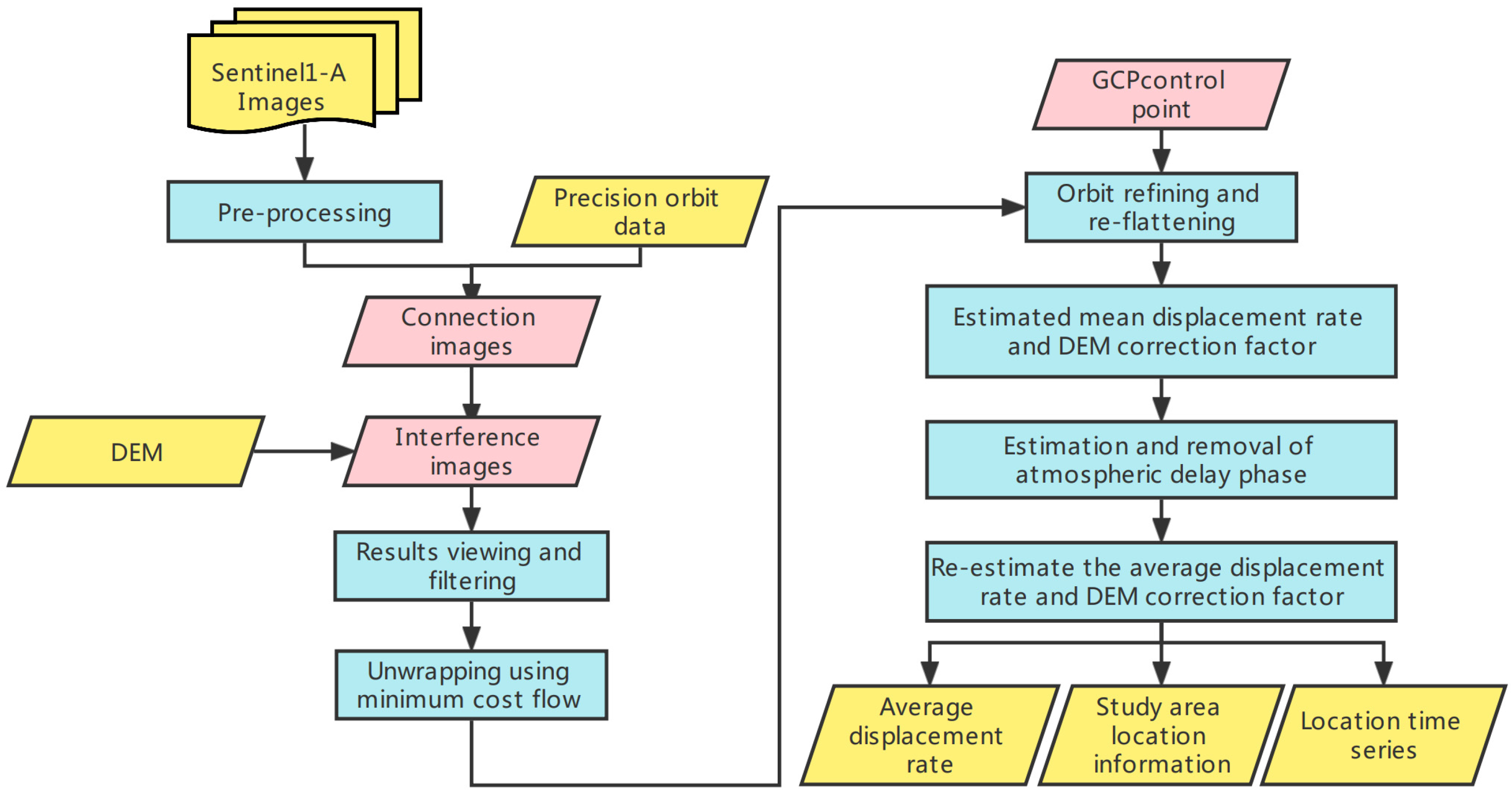
2.4. Principle of SBAS-InSAR

The basic principle of SBAS-InSAR is to sort all SAR images in temporal order ( t 1 ,   t 2 ,   ,   t k ), and to pair them. Next, the temporal baseline and spatial vertical baseline thresholds are set independently and the interferometric pairs smaller than the threshold are divided into one group, and so on. Finally, L sets of image pairs could be obtained [35]. For the i t h differential interferogram, assuming t 2 > t 1 , the expression of the differential interference phase is shown in Equation (2) [36]:
Φ i = Φ t 2 Φ t 1 4 π λ d t 2 d t 1 + 4 π λ × B i ξ R s i n θ + Φ a t m 2 Φ a t m 1 + Δ Φ
where Φ t 1 and Φ t 2 are the phases at moments t 1 and t 2 , respectively, d t 1 and d t 2 are the deformation relative to the reference image at moments t 1 and t 2 in the Line of Sight (LOS) direction of the satellite, B i is the vertical baseline, R is the distance from the satellite to the feature target, θ is the satellite incidence angle, λ is the radar wavelength, B i ξ R s i n θ is the residual terrain phase due to the inaccuracy of DEM, ( Φ a t m 2 Φ a t m 1 ) is the phase introduced by the atmospheric delay effect, and Δ Φ is the phase introduced by noise.
The linear model of linear deformation and DEM residual phase error in the study area can be expressed as:
T ,   M P = δ Φ  
where T is the time-dependent sparse matrix and M is the coefficient matrix associated with the spatial baseline. The linear deformation phase P can be expressed as:
P = v       ξ T  
where v is the linear deformation rate and ξ is the DEM error. The linear deformation rate can be obtained by solving the model, and the topographic error can be estimated.
The processing flow of SBAS-InSAR is shown in Figure 3.

2.5. Principles of Statistics–Time Series Prediction Models

Time series prediction models are mostly used in fields such as surface deformation, mainly by building models to predict future trends based on past data to provide guidance for future decisions. Holt′s exponential smoothing model is a classical forecasting model. Its advantage is that it can be used to smooth the factors of the original series with different parameters, which has a lot of flexibility and is especially suitable for data that vary continuously with time [37]. The Holt–Winters model can identify seasonality in time-series data. This model is applicable to non-stationary series containing linear trends and cyclical fluctuations, is widely used for short-term forecasting of future trends, and has provided excellent results [38]. ARIMA models are considered to be the most commonly used regression models for time-series forecasting in the last four decades [39] and are remarkable for fitting linearity without sacrificing trend predictions for long-term horizons. All of the three prediction models above have been proven to be effective for time-series prediction, and are applicable to the data in this paper; therefore, Holt′s exponential smoothing model, the Holt–Winters smoothing model, and the ARIMA model are selected for surface deformation prediction, and the prediction results are compared to obtain the model with the highest accuracy.

2.5.1. Holt′s Exponential Smoothing Model

Holt′s method retains both smoothing and trend information and can predict time-series data with trends. Its formulas at time t are as follows [40]:
L t = α Y t + 1 + α L t 1 + T t 1
T t = β L t L t 1 + 1 β T t 1
Y ^ t + m = L t + m T t
where, L t is the smoothed value, T t is the trend estimate, Y t is the observation value, Y ^ t + m is the forecast for m periods into the future; α and β are the smoothing constants for data and estimate, and m represents periods to be forecast in the future.

2.5.2. The Holt–Winters Smoothing Model

A series is said to have seasonal characteristics when a certain repeating pattern occurs at each fixed time interval, and this time interval is called a season. The Holt–Winters smoothing model predicts time series with trend and seasonality, and in this model, both the trend component and the seasonal component need to be smoothed exponentially. Its formulas at time t are as follows [41]:
L t = α x t s t s + 1 α L t 1 + T t 1
T t = β L t L t 1 + 1 β T t 1
S t = γ x t L t + 1 γ S t s
X ^ t + p = L t + p T t S t s + p
where, L t is the smoothed value or the current level estimate, T t is the trend estimate, S t is the seasonal estimate, x t is the observation value, X ^ t + p is forecast for p periods into the future; α , β , and γ are the smoothing constants for the level, trend, and seasonality estimate; p is the set time period to be predicted, and s is the length of the season, i.e., the length of a cycle.

2.5.3. ARIMA Model

The ARIMA model is established based on a smooth time series, which can effectively represent the linearity of the data and has a better short-term forecasting effect. Its formulas are as follows [42]:
Y ^ t = μ + Φ 1 × y t 1 + + Φ p × y t p + θ 1 × e t 1 + + θ q × e t q
where p is the lags of the time-series data itself in the model, also known as the AR/Auto-Regressive term; d is the order that needs to be differenced, also known as the integrated term; q is the lags of the prediction error, also known as the MA/Moving Average term; Φ is the coefficient of AR, and θ is the coefficient of MA.

2.6. Performance Indicators

In this paper, we use three common metrics, Mean Absolute Scaled Error (MASE) [43], Root Mean Squared Error (RMSE), and Mean Absolute Error (MAE) to reflect the predictive power of the model, which can be expressed by the following equations [44]:
M A S E = 1 j 0 j e j 1 T 1 t = 2 T y i y i 1
R M S E = 1 n i = 1 n y i y ^ i 2
M A E = 1 n i = 1 n y i y ^ i
where y , y i , and y ^ i represent the measured, predicted, and averaged values, respectively, e j is the error at the j -th iteration, and the training set is considered for time t ( t = 1 ,   2 ,   T ).

3. Results and Analysis

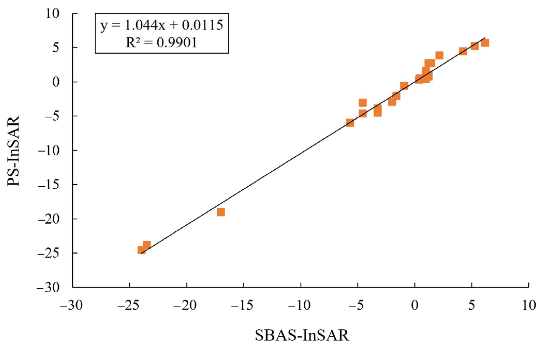
3.1. Cross-Validation of Monitoring Results

The surface deformation rate diagrams obtained by the two InSAR techniques are shown in Figure 4 and Figure 5, respectively. In order to verify the accuracy of the monitoring results, the results of PS-InSAR and SBAS-InSAR are cross-validated by a series of comparisons. Comparing the two figures, it can be seen that the distributions of the deformation rates of the two results are roughly the same, and both show the following salient features: the surface deformation motion in most of the study area shows subsidence, while a small part of the northeast area shows uplift; the distribution of the surface deformation rates in the study area is uneven, with the western and southeastern areas showing relatively low deformation rates and stable surface movement, and slow subsidence, while the regions in the northwestern and southwestern areas show slightly higher subsidence rates.
For a more accurate analysis, 26 randomly selected deformation monitoring points in the study area were randomly selected as sample points in this paper, and the PS-InSAR and SBAS-InSAR deformation rate monitoring values of these points were compared. The comparison results are shown in Table 1, below. In addition, a Pearson correlation analysis and linear regression analysis were performed on the sample points, and the results are shown in Figure 6. From the statistical results in Table 1, the relative errors of PS-InSAR and SBAS-InSAR results are within 3 mm/a, mostly within 0.5 mm/a, and the absolute mean value is 0.65 mm/a. Figure 6 shows that the correlation coefficient of the sample points is 0.995 and R² = 0.9901. It indicates that the results obtained by PS-InSAR and SBAS-InSAR are relatively consistent, and the monitoring results are relatively reliable.

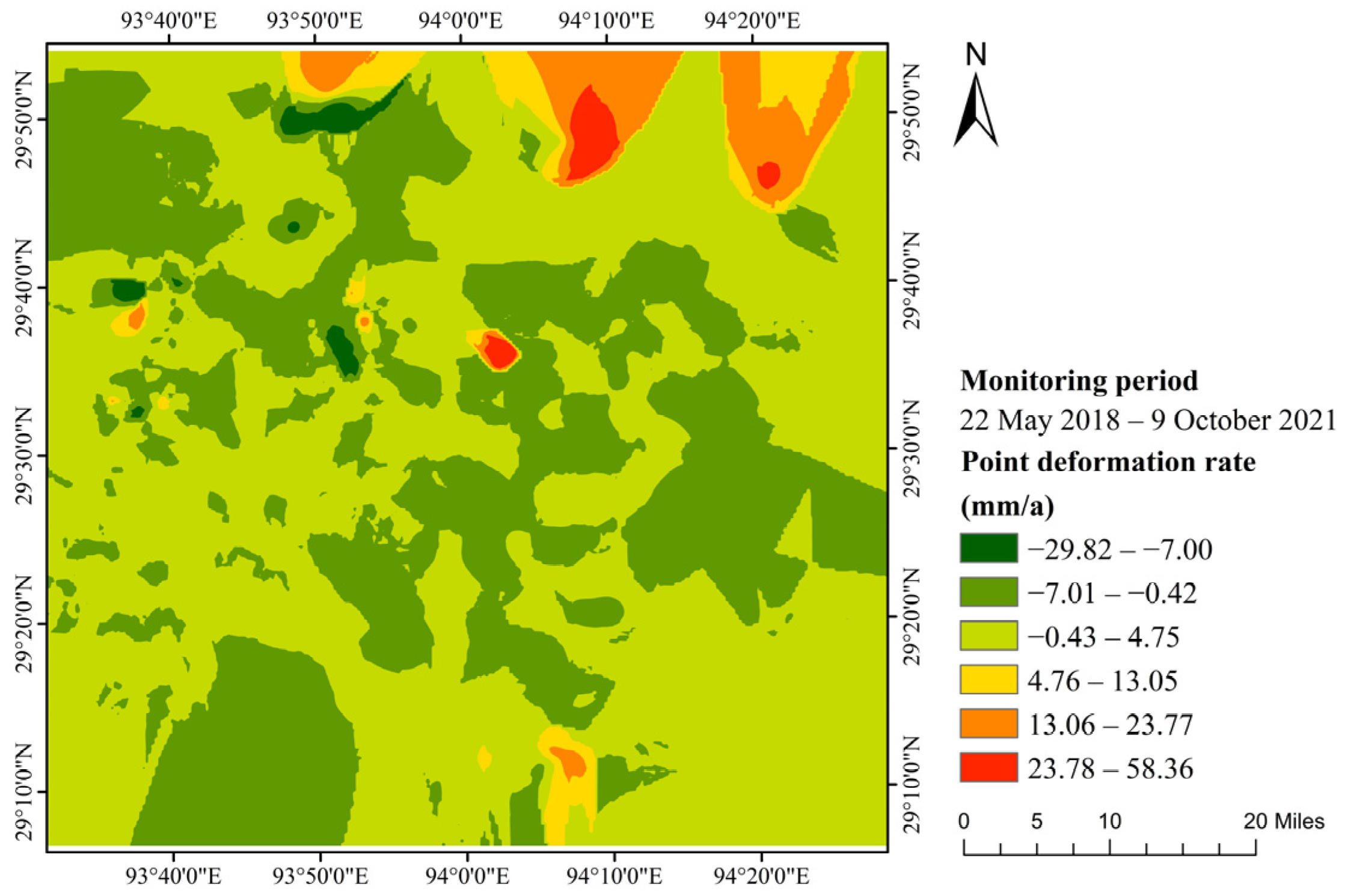
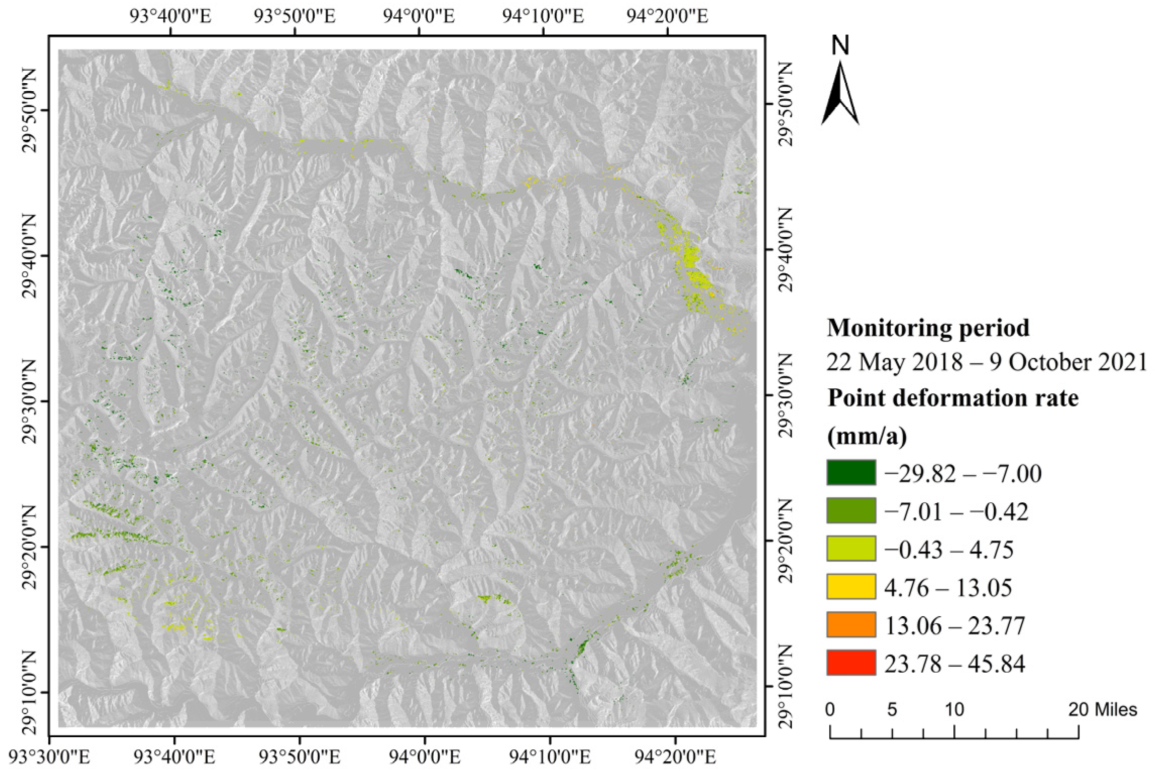
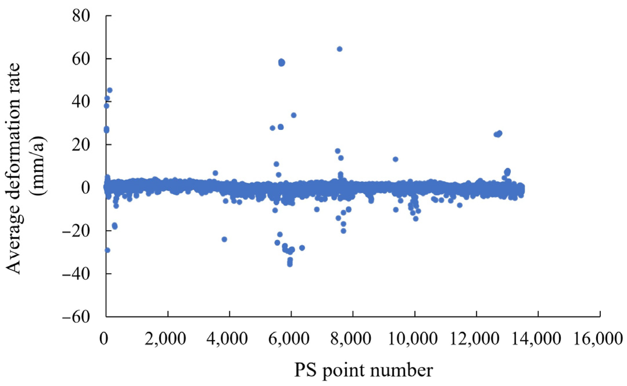
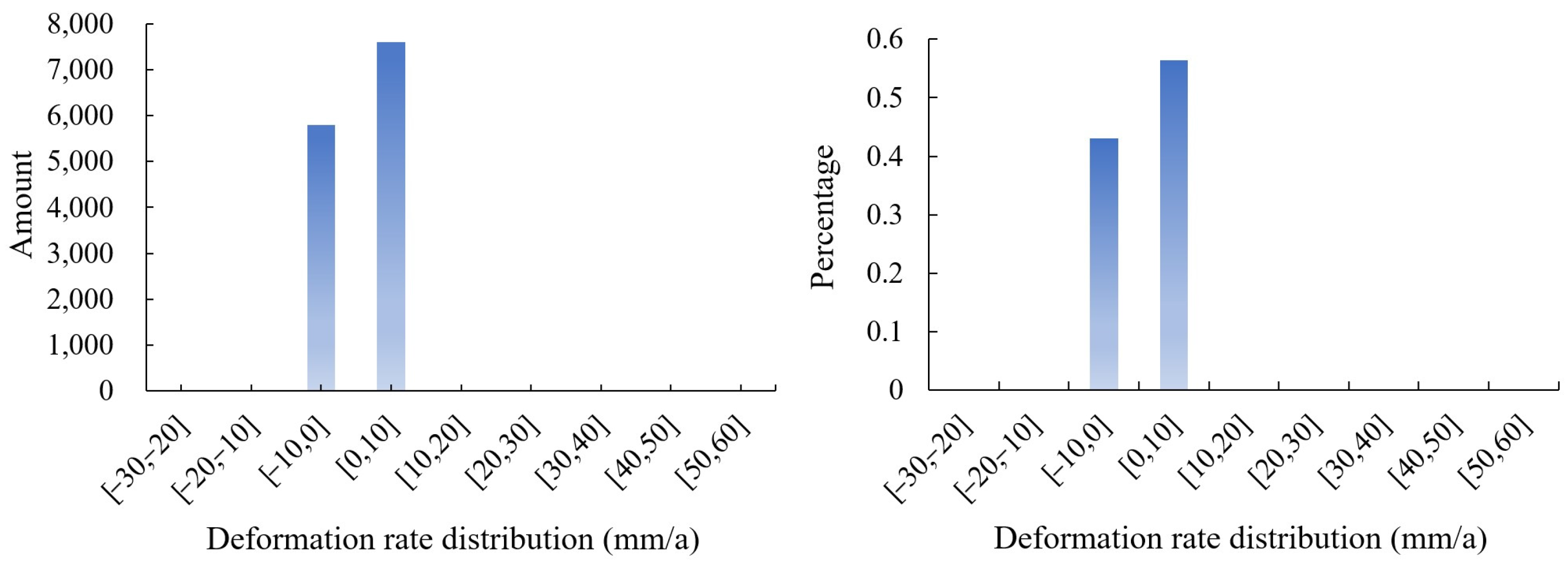
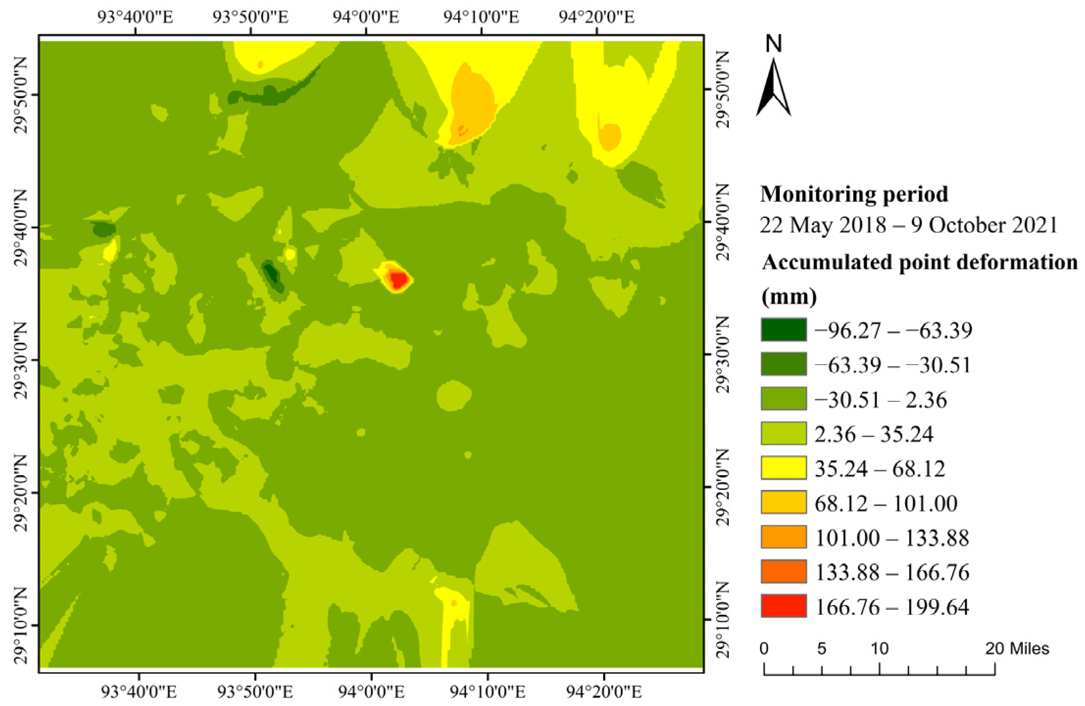
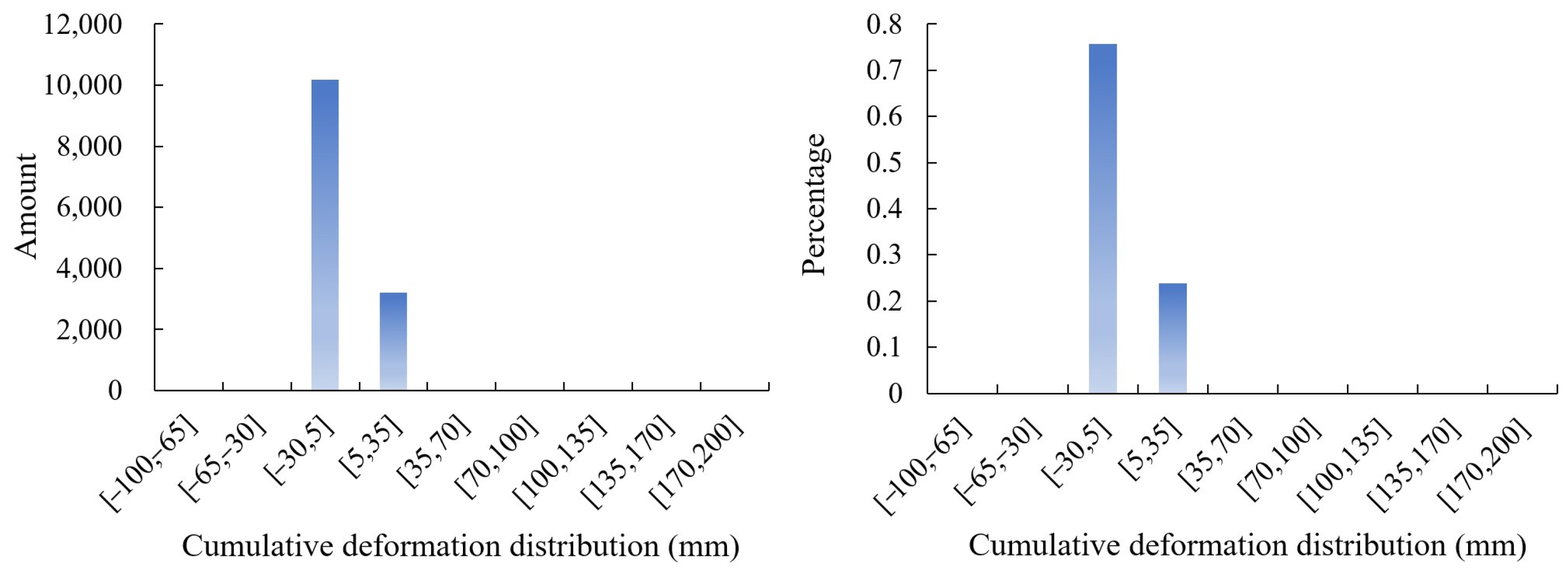
3.2. Analysis of Surface Deformation Monitoring Results

The comparison of the two time-series InSAR results shows that the density of deformation points extracted based on PS-InSAR is higher than that of SBAS-InSAR, so the PS-InSAR results are analyzed in this paper as the main results, and SBAS-InSAR as the auxiliary results.
Statistically, there are 13,483 monitoring points in the study area, and the distribution of the deformation rate is shown in Figure 5 and Figure 7. It can be observed that the areas with severe deformation are mainly centered in a small part of the northwest, northeast, and central parts, with the maximum subsidence rate at 29.42 mm/a and the maximum uplift rate at 58.27 mm/a. The values of the deformation rate are mostly distributed in the range (−20, 20), and the deformation rate of most of the monitoring points in this range is close to 0.
Figure 8 displays the bar chart for the deformation rate. From the histogram, the deformation rate is mainly distributed in the ranges (−10, 0) and (0, 10), with 5801 and 7599 control points distributed, respectively, accounting for about 43% and 56% of the total number of control points. In the rest of the deformation rate ranges, the difference between the number and proportion of control points is small, and the numbers are all lower than 1000, accounting for less than 10% of the control points. The above results indicate that the surface deformation in the research region is dominated by slow deformation.
Figure 9 shows the distribution of the cumulative deformation value of the ground points, and Figure 10 statistically shows the distribution ranges of the cumulative deformation of the ground points. As can be seen from the figures in the study area, the maximum cumulative subsidence reaches 96.27 mm, and the maximum cumulative uplift reaches 199.64 mm; the cumulative deformation in most of the areas shows subsidence, and only some areas in the north and central parts show uplift. The cumulative deformation range with the largest number of ground points is (−30, 5), and the number of ground points accounts for about 76% of the total; the second is the range (5, 35), and the number of ground points accounts for about 24% of the total.

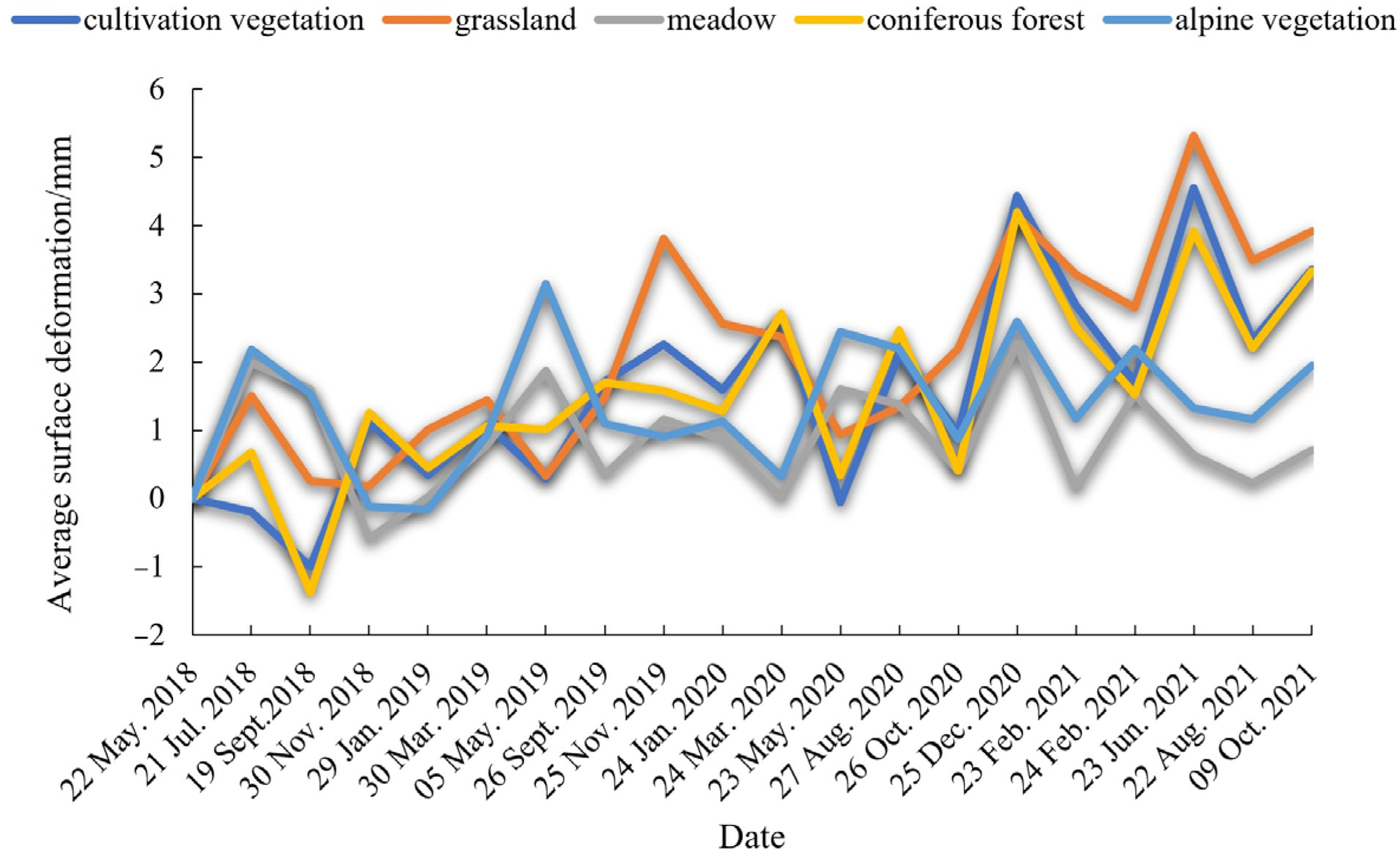
3.3. Results of Surface Deformation under Different Vegetation Types

Figure 11 shows the average cumulative surface deformation results for monitoring sites located within different vegetation types at 20 time points during the monitoring period. The results show that the surface deformation of each vegetation type exhibits a certain periodicity, which is generally consistent with the pattern of seasonal permafrost melting in summer and freezing in winter. Among them, the deformation trends of the meadow and alpine vegetation are similar and remain stable overall, without showing obvious uplifting or subsidence trends; the deformation trends of the cultivated vegetation, grassland, and coniferous forest are similar, with more drastic deformation and an overall uplifting trend.

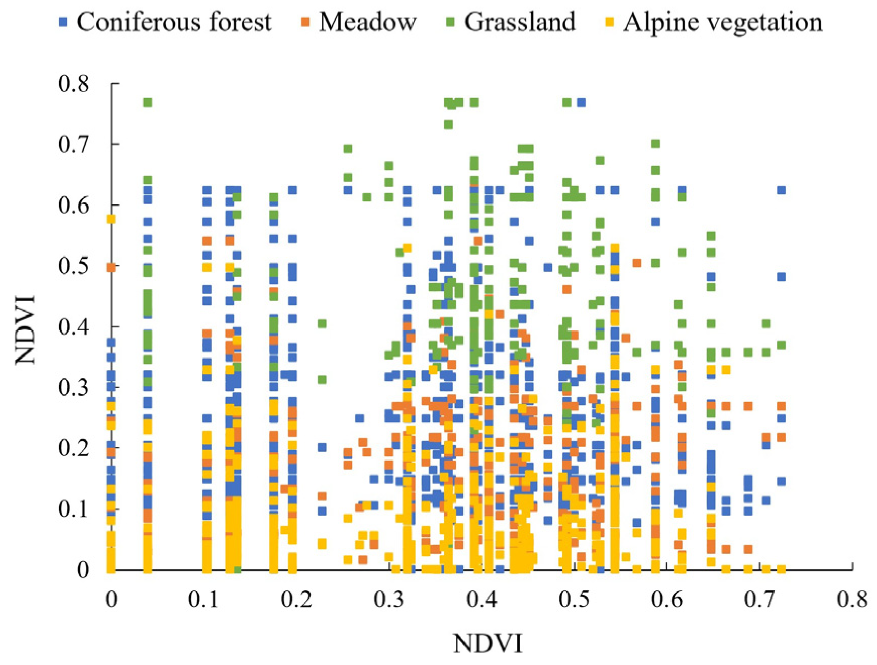
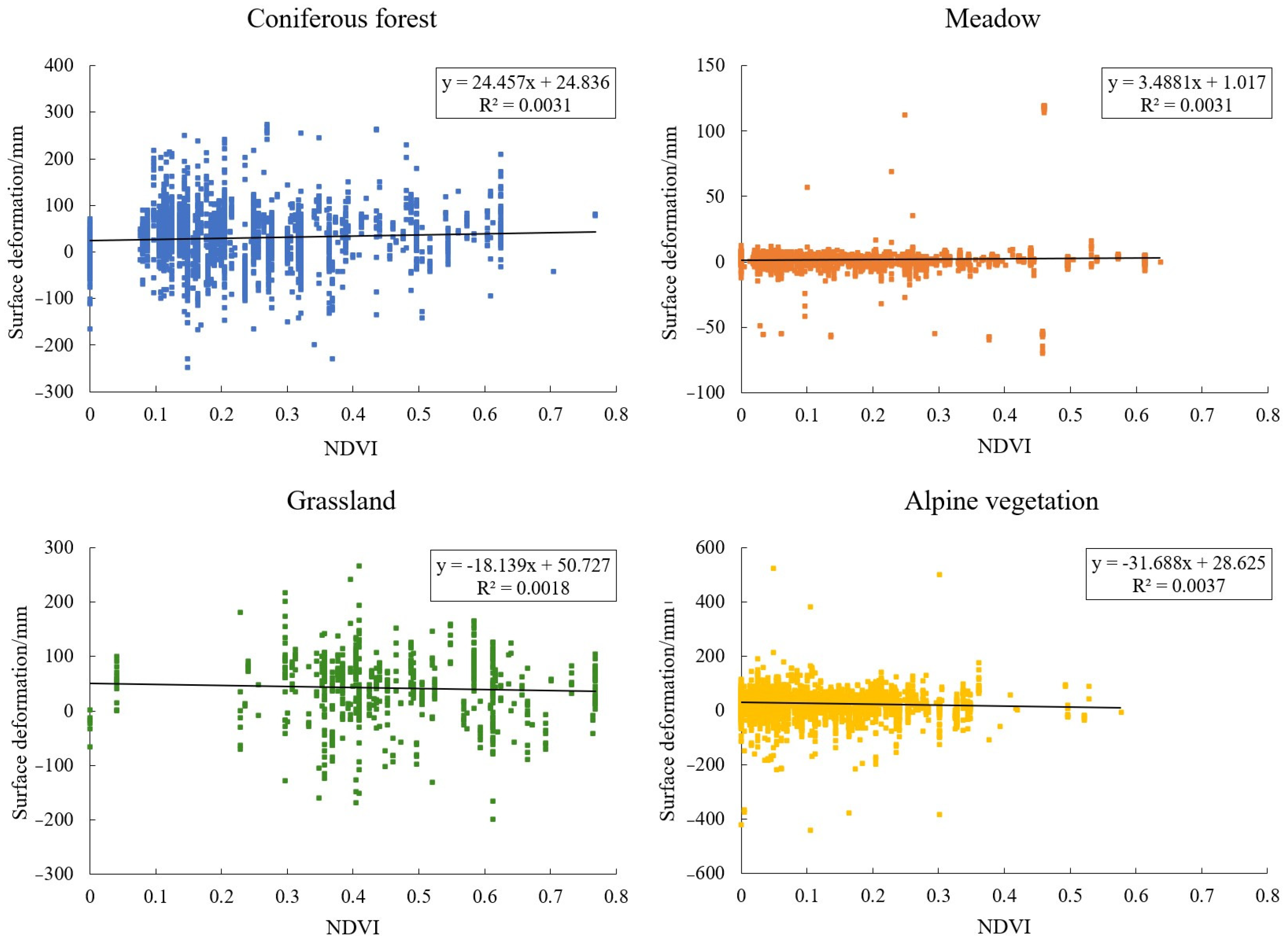
3.4. Correlation between Permafrost Deformation and Normalized Vegetation Index

It has been confirmed that the vegetation cover of an ecosystem can be expressed by the normalized vegetation index (NDVI) [45,46,47]. This paper correlates and regresses surface deformation measurements with the NDVI of the monitoring sites to quantify the link between permafrost deformation and vegetation. The monitoring sites are divided into five categories according to the vegetation cover types, because there are differences in permafrost deformation among the various vegetation cover types in the study area, and these differences significantly affect the correlation relationships and regression relationships between permafrost deformation and NDVI. Firstly, the Pearson correlation coefficient and significance level between surface deformation and NDVI at the monitoring sites were calculated using SPSS software. It is generally accepted that a less than 0.05 significance test result indicates that the results are statistically significant and are not the consequence of sampling error. The calculated results are shown in Table 2.
From the results, NDVI and permafrost deformation are significantly correlated (p < 0.01) in areas with the vegetation cover types of grassland, meadow, alpine vegetation, and coniferous forest. For the types with significant correlation, we further applied regression analysis to explore the role between NDVI and surface deformation, and the NDVI distribution and regression analysis results for these areas are shown in Figure 12 and Figure 13, respectively.

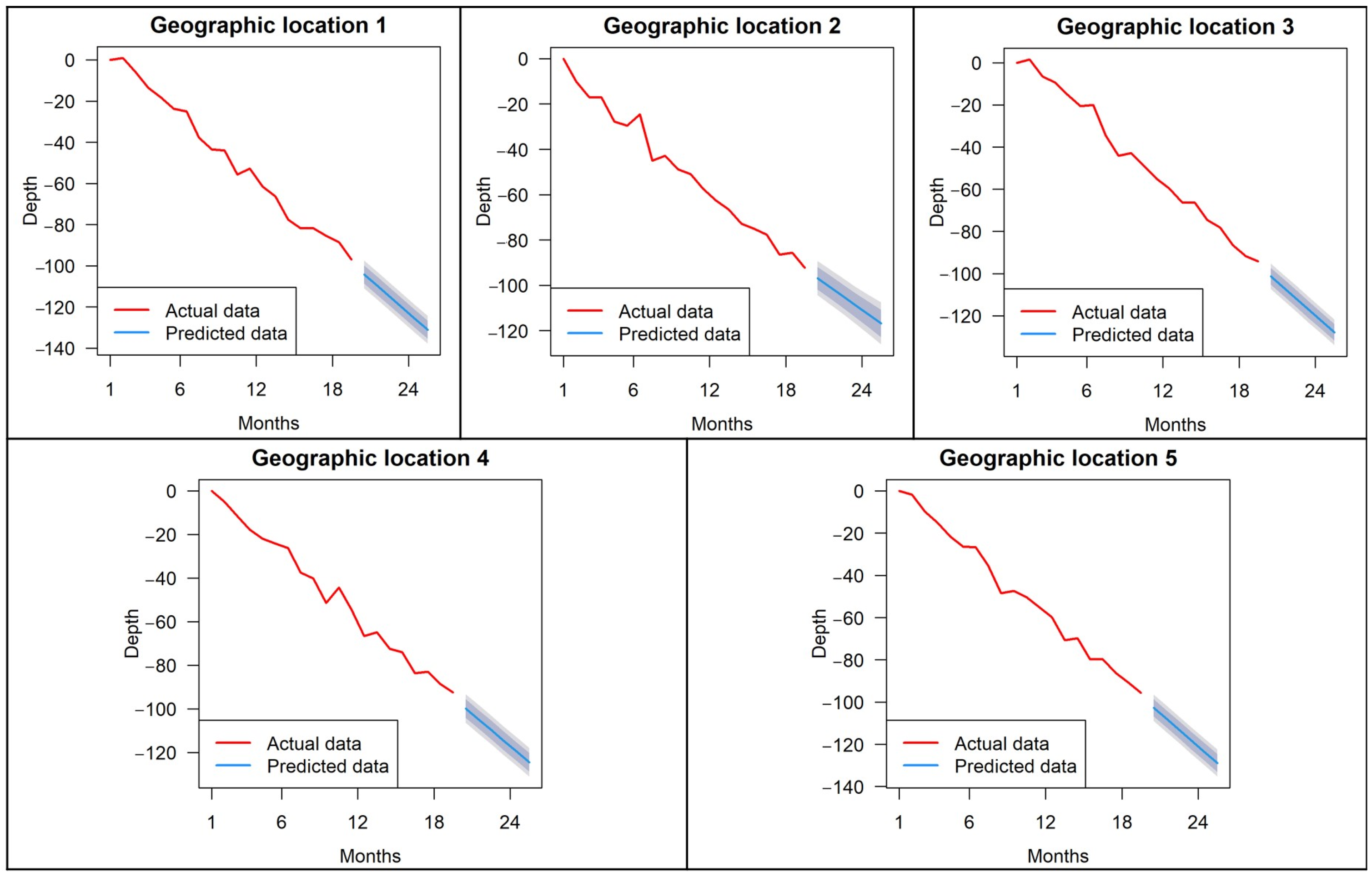
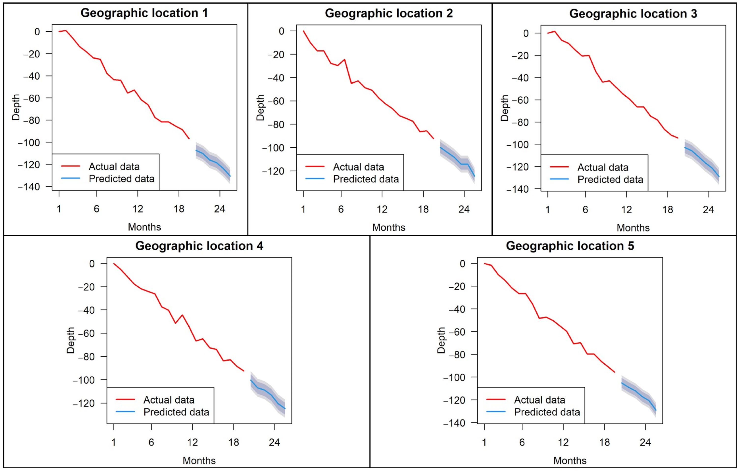
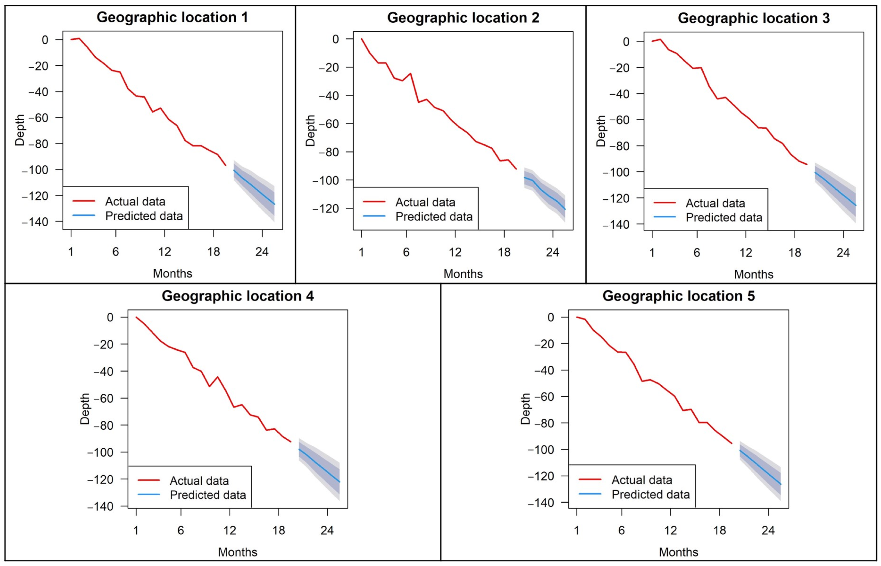
3.5. Comparative Analysis of Machine Learning Prediction Models

In this paper, based on the surface deformation monitoring results obtained from PS-InSAR, five PS points were randomly selected as sample points and the Holt′s exponential smoothing model, the Holt–Winters smoothing model, and the ARIMA model in the statistical time-series model were used to predict surface deformation for these five points, and by comparing the relevant indexes and prediction effects, the most applicable model in this study was obtained. In this paper, three accuracy indicators are used to assess the reliability of the model, all three of which are widely used to reflect the error in the predicted values [48,49,50,51]. In our evaluation of the test data with MASE, a value of lower than one implicates a better mean average error [52,53]. When MASE is less than one, the smaller the MASE, RMSE, and MAE, the smaller the error of the model and the higher the accuracy of the prediction.
The prediction is set for the next six months, and since the time interval of the time-series data in this paper is one month, predicting six months will result in three sets of data. The results are shown in Figure 14, Figure 15 and Figure 16. The prediction lines in the figure have an 80 percent confidence interval shaded in blue and a 95 percent confidence interval shaded in gray.
From Figure 14, Figure 15 and Figure 16, and Table 3, it can be seen that the average MASE of all three models is much less than 1. The average RMSE of the Holt′s smoothing model prediction results is 3.2092, the average MAE is 2.5376, and the average MASE is 0.0702; the average RMSE of the Holt–Winters smoothing model prediction results is 2.9938, the average MAE is 2.1039, and the average MASE is 0.0644; the average RMSE of the ARIMA model prediction results is 3.0938, the average MAE is 2.378, and the average MASE is 0.065. After comparison, all three indicators of the Holt–Winters smoothing model prediction results are better than the Holt′s model and the ARIMA model, so it can be concluded that this model has the highest prediction accuracy and is most suitable for the prediction of future surface deformation in the study area.

4. Discussion

4.1. Correlation Analysis of Vegetation Type and Surface Deformation

As shown in Figure 11, the surface deformation patterns under cultivated vegetation, grassland, and coniferous forest conditions showed some similarity during the monitoring period, and showed a small uplift trend on the whole, unlike the surface deformation under meadow and alpine vegetation conditions, which remained at a relatively stable level. The distribution of cultivated vegetation, grassland, and coniferous forest overlaps with residential areas, as can be observed from the examination of the actual situation in the research region; therefore, the surface deformation in these types of vegetation-covered areas is not only related to permafrost, but various human activities are also one of the influencing factors [54,55,56,57,58,59], such as road construction and housing renovation, etc. It can be assumed that the surface uplift may be related to these anthropogenic influences based on the findings of monitoring surface deformation in places with active human activity, such as cities.
Vegetation has two important functions for permafrost, namely the insulation function and the cooling function. In summer, vegetation partially blocks solar radiation and cools the soil, while in winter, vegetation can block soil heat dissipation and play an insulating role for the soil. Different vegetation covers have different degrees of influence on water and heat transport, and the freeze-thaw processes, and have different functions on permafrost. Among the five vegetation cover types included in the study area, there are significant correlations between the surface deformation phenomena of grassland, meadow, coniferous forest, and alpine vegetation, and NDVI, among which the surface deformation of grassland and alpine vegetation is negatively correlated with NDVI, and the surface deformation of meadow and the coniferous forest is positively correlated with NDVI. This finding can support the idea that permafrost and plants are closely related and interact with one another through changes in soil heat and moisture conditions [60,61,62]. With the increase in grassland and alpine vegetation cover, the surface deformation shows a subsiding trend, and it can be seen that grassland and alpine vegetation are dominated by heat preservation. With the increase in the meadow and coniferous forest cover, the surface deformation tends to rise, and it can be seen that meadow and coniferous forest mainly play a cooling role. In addition, alpine vegetation, coniferous forest, and grassland have a stronger effect on surface deformation, while meadows are weaker.

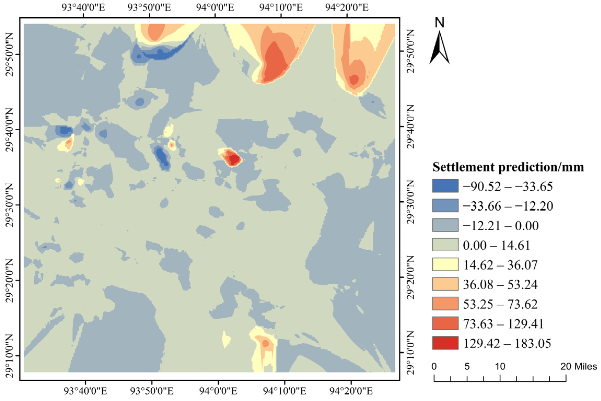
4.2. Spatial Distribution of Surface Deformation Predictions

According to the conclusion obtained above, the Holt–Winters smoothing model is the most accurate model. Therefore, the Holt–Winters smoothing model was used to estimate the surface deformation in the study region over the following two months based on the deformation findings acquired using the PS-InSAR technique, and the results are given in Figure 17. The findings indicate that the study area′s maximum cumulative subsidence and uplift are predicted to reach 90.52 mm and 183.1 mm, both of which are slightly lower than the actual monitored values; in addition, the area of the uplifted zone increases, while the area of the severely subsided zone and the degree of subsidence decreases.
In general, the surface deformation trend in the study area did not change drastically, and the surface deformation activity in most areas showed a continuous uplift. The possible reason for this prediction result is that, according to the existing studies on the seasonal permafrost depth changes in Tibetan areas, October to December is the period of the year when the active layer of permafrost gradually starts to freeze, and when the permafrost begins to thaw in the April of the following year [63,64,65]. In this paper, the prediction period is from October to December 2021, which is in the period of permafrost freezing by the law of seasonal permafrost freezing and thawing, so the surface deformation in the prediction results shows extensive uplift.
The surface deformation will exhibit various trends depending on the vegetation cover. In this paper, the average values of the predicted and actual values of cumulative surface deformation for each of the five vegetation types were calculated and compared, and the results are shown in Figure 18. In the next two months, the surface deformation of the five vegetation types will show an uplift, among which the uplift of alpine vegetation and coniferous forest is small, at less than 0.1 mm, while the surface deformation of the meadow, grassland, and cultivated vegetation will show a relatively large uplift. The prediction of surface deformation in the permafrost area can provide a data reference for the rational arrangement of agricultural production, engineering construction, and other activities, and help in the prevention and mitigation of surface deformation disasters; meanwhile, the prediction technique can also provide technical support for future ecological construction planning in the Tibetan permafrost area. For example, the predicted results can be used as one of the influence factors to support the prediction of the area evolution of each vegetation type in the permafrost area. After obtaining the subsurface soil organic carbon contents for different vegetation type conditions, the predicted results of vegetation distribution can further support the prediction of soil organic carbon storage in the permafrost area [66]. This result can help in taking timely ecological restoration measures for areas with a low soil carbon content and help to promote the enhancement of the carbon sink capacity of ecosystems.

4.3. Research Limitations and Future Directions

Due to the complexity of the topographic environment in the study area and the limitations of the radar remote sensing technology, there are still some shortcomings in this study, mainly that the interferometric phase accuracy in the vegetation area needs to be improved. Environmental factors determine the observation conditions of SAR satellites. The study area of this paper is in a high-altitude mountainous area with dense vegetation cover and is covered with snow and ice all year round, which easily leads to such phenomena as low coherence and out-of-coherence, affecting the effect and accuracy of InSAR deformation inversion. In future studies, we will try to use data sets with higher spatial resolution, extend monitoring periods, shorten monitoring intervals, or try to develop new interferometric methods to improve the applicability of InSAR in areas with high vegetation cover.

5. Conclusions

(1) Surface deformation in the study area was mainly slow subsidence, with 98% of the ground control points having a deformation rate within the interval (−10, 10), with a maximum subsidence rate of 29.42 mm/a and a maximum uplift rate of 58.27 mm/a over the monitoring time period; 76% of the ground control points had a cumulative deformation within the interval (−30, 5), with a maximum cumulative subsidence of 96.27 mm and a maximum cumulative uplift of 199.64 mm over the monitoring time period. This indicates that the magnitude of surface deformation is relatively small in most of the study area, and the active layer of permafrost exhibits seasonal freezing and thawing.
(2) The analysis of permafrost deformation in different vegetation cover areas of the study area showed that the surface deformation of each vegetation type showed a certain periodicity, among which the surface deformation of grassland and alpine vegetation was negatively correlated with NDVI, while the surface deformation of meadow and coniferous forest was positively correlated with NDVI. In addition, the regression analysis showed that the influence of grassland, coniferous forest, and alpine vegetation on surface deformation was stronger than that of meadow. The above results show that the higher vegetation cover of grassland and alpine vegetation has a stronger insulating effect on permafrost, leading to ground subsidence, while the higher vegetation cover of meadow and coniferous forest has a stronger cooling effect on permafrost, leading to surface uplift. Meanwhile, alpine vegetation, coniferous forests, and grasslands have stronger insulation and cooling effects on permafrost, and the meadows are weaker.
(3) Among the three machine learning prediction models selected, the Holt–Winters smoothing model was the model with the highest prediction accuracy. The surface deformation activity showed an uplift in most areas, according to the prediction results of this model, while the area and degree of subsidence decreased. Among the five vegetation types, the difference between the predicted and actual values of surface deformation under alpine vegetation and coniferous forest conditions was smaller than those of grassland, meadow, and cultivated vegetation, with the smallest difference being for alpine vegetation and the largest difference being for cultivated vegetation. The above results reflect that in the Tibetan tundra, the better the vegetation growth, the more stable the permafrost will be, and the higher the stability of the ecosystem.

Author Contributions

X.W. performed data treatments and wrote the paper; W.L., J.M., L.Y., and J.L. contributed to the discussion of the results; Q.Y. contributed some ideas and revised the paper; All authors edited the paper. All authors have read and agreed to the published version of the manuscript.

Funding

This research was funded by the National Natural Science Foundation of China Youth Science Foundation Project, grant number 42001211.

Data Availability Statement

Publicly available datasets were analyzed in this study. The data sources are indicated in the text.

Acknowledgments

We thank Beijing Forestry University, College of Forestry for support to the authors. In addition, we thank the reviewers for their valuable suggestions that helped to improve the quality of the manuscript.

Conflicts of Interest

The authors declare no conflict of interest.

References

  1. Adhikari, K.; Owens, P.R.; Libohova, Z.; Miller, D.M.; Wills, S.A.; Nemecek, J. Assessing Soil Organic Carbon Stock of Wisconsin, USA and Its Fate under Future Land Use and Climate Change. Sci. Total Environ. 2019, 667, 833–845. [Google Scholar] [CrossRef] [PubMed]
  2. Wang, J.; He, G.; Fang, H.; Han, Y. Climate Change Impacts on the Topography and Ecological Environment of the Wetlands in the Middle Reaches of the Yarlung Zangbo-Brahmaputra River. J. Hydrol. 2020, 590, 125419. [Google Scholar] [CrossRef]
  3. Ma, F.; Chen, J.; Chen, J.; Wang, T.; Yan, J. Evolution of the Hydro-Ecological Environment and Its Natural and Anthropogenic Causes during 1985–2019 in the Nenjiang River Basin. Sci. Total Environ. 2021, 799, 149256. [Google Scholar] [CrossRef]
  4. Buonocore, C.; Pascual, J.; Cayeiro, M.; Salinas, R.M.; Mejías, M.B. Modelling the Impacts of Climate and Land Use Changes on Water Quality in the Guadiana Basin and the Adjacent Coastal Area. Sci. Total Environ. 2021, 776, 146034. [Google Scholar] [CrossRef]
  5. Jiang, C.; Wang, F.; Zhang, H.; Dong, X. Quantifying Changes in Multiple Ecosystem Services during 2000–2012 on the Loess Plateau, China, as a Result of Climate Variability and Ecological Restoration. Ecol. Eng. 2016, 97, 258–271. [Google Scholar] [CrossRef]
  6. Luo, D.; Jin, H.; Bense, V.F. Ground Surface Temperature and the Detection of Permafrost in the Rugged Topography on NE Qinghai-Tibet Plateau. Geoderma 2019, 333, 57–68. [Google Scholar] [CrossRef]
  7. Bosch, A.; Schmidt, K.; He, J.S.; Doerfer, C.; Scholten, T. Potential CO2 Emissions from Defrosting Permafrost Soils of the Qinghai-Tibet Plateau under Different Scenarios of Climate Change in 2050 and 2070. Catena 2017, 149, 221–231. [Google Scholar] [CrossRef]
  8. Wang, T.; Wu, T.; Wang, P.; Li, R.; Xie, C.; Zou, D. Spatial Distribution and Changes of Permafrost on the Qinghai-Tibet Plateau Revealed by Statistical Models during the Period of 1980 to 2010. Sci. Total Environ. 2019, 650, 661–670. [Google Scholar] [CrossRef]
  9. Wang, G.; Mao, T.; Chang, J.; Song, C.; Huang, K. Processes of Runoff Generation Operating during the Spring and Autumn Seasons in a Permafrost Catchment on Semi-Arid Plateaus. J. Hydrol. 2017, 550, 307–317. [Google Scholar] [CrossRef]
  10. Lin, Z.; Gao, Z.; Niu, F.; Luo, J.; Yin, G.; Liu, M.; Fan, X. High Spatial Density Ground Thermal Measurements in a Warming Permafrost Region, Beiluhe Basin, Qinghai-Tibet Plateau. Geomorphology 2019, 340, 1–14. [Google Scholar] [CrossRef]
  11. Sun, A.; Zhou, J.; Yu, Z.; Jin, H.; Sheng, Y.; Yang, C. Three-Dimensional Distribution of Permafrost and Responses to Increasing Air Temperatures in the Head Waters of the Yellow River in High Asia. Sci. Total Environ. 2019, 666, 321–336. [Google Scholar] [CrossRef] [PubMed]
  12. Chen, J.; Wu, Y.; O’Connor, M.; Cardenas, M.B.; Kling, G. Active Layer Freeze-Thaw and Water Storage Dynamics in Permafrost Environments Inferred from InSAR. Remote Sens. Environ. 2020, 248, 112007. [Google Scholar] [CrossRef]
  13. Li, D.; Wen, Z.; Luo, J.; Zhang, M.; Chen, B. Slope Failure Induced by Cold Snap and Continuous Precipitation in the Seasonal Frozen Area of Qinghai-Tibet Plateau. Sci. Total Environ. 2019, 694, 133547.1–133547.10. [Google Scholar] [CrossRef] [PubMed]
  14. Shang, W.; Wu, X.; Zhao, L.; Yue, G.; Zhao, Y.; Qiao, Y.; Li, Y. Seasonal Variations in Labile Soil Organic Matter Fractions in Permafrost Soils with Different Vegetation Types in the Central Qinghai–Tibet Plateau. Catena 2016, 137, 670–678. [Google Scholar] [CrossRef]
  15. Liu, Z.; Chen, B.; Wang, S.; Wang, Q.; Chen, J.; Shi, W.; Wang, X.; Liu, Y.; Tu, Y.; Huang, M.; et al. The Impacts of Vegetation on the Soil Surface Freezing-Thawing Processes at Permafrost Southern Edge Simulated by an Improved Process-Based Ecosystem Model. Ecol. Model. 2021, 456, 109663. [Google Scholar] [CrossRef]
  16. Jin, X.-Y.; Jin, H.-J.; Iwahana, G.; Marchenko, S.S.; Luo, D.-L.; Li, X.-Y.; Liang, S.-H. Impacts of Climate-Induced Permafrost Degradation on Vegetation: A Review. Adv. Clim. Chang. Res. 2021, 12, 29–47. [Google Scholar] [CrossRef]
  17. Guo, W.; Liu, H.; Anenkhonov, O.A.; Shangguan, H.; Sandanov, D.V.; Korolyuk, A.Y.; Hu, G.; Wu, X. Vegetation Can Strongly Regulate Permafrost Degradation at Its Southern Edge through Changing Surface Freeze-Thaw Processes. Agric. For. Meteorol. 2018, 252, 10–17. [Google Scholar] [CrossRef]
  18. Yang, Y.; Wu, Z.; Guo, L.; He, H.S.; Li, M.H. Effects of Winter Chilling vs. Spring Forcing on the Spring Phenology of Trees in a Cold Region and a Warmer Reference Region. Sci. Total Environ. 2020, 725, 138323. [Google Scholar] [CrossRef]
  19. Xiao, G.; Zhang, Q.; Yu, L.; Wang, R.; Bai, H. Impact of Temperature Increase on the Yield of Winter Wheat at Low and High Altitudes in Semiarid Northwestern China. Agric. Water Manag. 2010, 97, 1360–1364. [Google Scholar] [CrossRef]
  20. Saulnier, M.; Talon, B.; Edouard, J.L. New Pedoanthracological Data for the Long-Term History of Forest Species at Mid-High Altitudes in the Queyras Valley (Inner Alps). Quat. Int. 2015, 366, 15–24. [Google Scholar] [CrossRef]
  21. Zhang, B.; Niu, Z.; Zhang, D.; Huo, X. Dynamic Changes and Driving Forces of Alpine Wetlands on the Qinghai–Tibetan Plateau Based on Long-Term Time Series Satellite Data: A Case Study in the Gansu Maqu Wetlands. Remote Sens. 2022, 14, 4147. [Google Scholar] [CrossRef]
  22. Liu, X.; Chen, Y.; Li, Z.; Li, Y.; Zhang, Q.; Zan, M. Driving Forces of the Changes in Vegetation Phenology in the Qinghai–Tibet Plateau. Remote Sens. 2021, 13, 4952. [Google Scholar] [CrossRef]
  23. Su, X.; Zhang, Y.; Jia, J.; Liang, Y.; Li, Y. InSAR-Based Monitoring and Identification of Potential Landslides in Lueyang County, the Southern Qinling Mountains, China. J. Mt. Sci. 2021, 39, 59–70. [Google Scholar] [CrossRef]
  24. Meng, Z.; Shu, C.; Wu, Q.; Yang, Y.; Fu, Z. Monitoring Surface Deformation of High-Speed Railway Using Time-Series InSAR Method in Northeast China. IOP Conf. Ser. Earth Environ. Sci. 2021, 660, 012011. [Google Scholar] [CrossRef]
  25. Yao, J.; Yao, X.; Wu, Z.; Liu, X. Research on Surface Deformation of Ordos Coal Mining Area by Integrating Multitemporal D-InSAR and Offset Tracking Technology. J. Sens. 2021, 2021, 1–14. [Google Scholar] [CrossRef]
  26. Jiang, C.; Fan, W.; Yu, N.; Nan, Y. A New Method to Predict Gully Head Erosion in the Loess Plateau of China Based on SBAS-InSAR. Remote Sens. 2021, 13, 421. [Google Scholar] [CrossRef]
  27. Cian, F.; Blasco, J.M.D.; Carrera, L. Sentinel-1 for Monitoring Land Subsidence of Coastal Cities in Africa Using PSInSAR: A Methodology Based on the Integration of SNAP and StaMPS. Geosciences 2019, 9, 124. [Google Scholar] [CrossRef]
  28. Li, H.; Zhu, L.; Dai, Z.; Gong, H.; Guo, T.; Guo, G.; Wang, J.; Teatini, P. Spatiotemporal Modeling of Land Subsidence Using a Geographically Weighted Deep Learning Method Based on PS-InSAR. Sci. Total Environ. 2021, 799, 149–244. [Google Scholar] [CrossRef]
  29. Chen, J.; Wu, T.; Zou, D.; Liu, L.; Wu, X.; Gong, W.; Zhu, X.; Li, R.; Hao, J.; Hu, G.; et al. Magnitudes and Patterns of Large-Scale Permafrost Ground Deformation Revealed by Sentinel-1 InSAR on the Central Qinghai-Tibet Plateau. Remote Sens. Environ. 2022, 268, 112778. [Google Scholar] [CrossRef]
  30. Zhao, R.; Li, Z.; Feng, G.; Wang, Q.; Hu, J. Monitoring Surface Deformation over Permafrost with an Improved SBAS-InSAR Algorithm: With Emphasis on Climatic Factors Modeling. Remote Sens. Environ. 2016, 184, 276–287. [Google Scholar] [CrossRef]
  31. Rouyet, L.; Lauknes, T.R.; Christiansen, H.H.; Strand, S.M.; Larsen, Y. Seasonal Dynamics of a Permafrost Landscape, Adventdalen, Svalbard, Investigated by InSAR. Remote Sens. Environ. 2019, 231, 111236. [Google Scholar] [CrossRef]
  32. Ran, Y.; Li, X.; Cheng, G.; Zhang, T.; Wu, Q.; Jin, H.; Jin, R. Distribution of Permafrost in China: An Overview of Existing Permafrost Maps. Permafr. Periglac. Processes 2012, 23, 322–333. [Google Scholar] [CrossRef]
  33. Mu’Amalah, A.; Anjasmara, I.M.; Taufik, M. Land Subsidence Monitoring in Cepu Block Area Using PS-Insar Technique. IOP Conf. Ser. Earth Environ. Sci. 2021, 731, 012011. [Google Scholar] [CrossRef]
  34. Khan, R.; Li, H.; Afzal, Z.; Basir, M.; Arif, M.; Hassan, W. Monitoring Subsidence in Urban Area by PSInSAR: A Case Study of Abbottabad City, Northern Pakistan. Remote Sens. 2021, 13, 1651. [Google Scholar] [CrossRef]
  35. Chen, Y.; Tong, Y.; Tan, K. Coal Mining Deformation Monitoring Using SBAS-InSAR and Offset Tracking: A Case Study of Yu County, China. IEEE J. Sel. Top. Appl. Earth Obs. Remote Sens. 2020, 13, 6077–6087. [Google Scholar] [CrossRef]
  36. Yang, Y.; Sun, Y.; Wu, S.; Dong, X.; Meng, Z. Surface Deformation Monitoring of a Section of Gongyu Expressway Based on SBAS-InSAR Technology. E3S Web Conf. 2021, 233, 01149. [Google Scholar] [CrossRef]
  37. Leenawong, C.; Chaikajonwat, T. Event Forecasting for Thailand’s Car Sales during the COVID-19 Pandemic. Data 2022, 7, 86. [Google Scholar] [CrossRef]
  38. Almazrouee, A.I.; Almeshal, A.M.; Almutairi, A.S.; Alenezi, M.R.; Alhajeri, S.N.; Alshammari, F.M. Forecasting of Electrical Generation Using Prophet and Multiple Seasonality of Holt–Winters Models: A Case Study of Kuwait. Appl. Sci. 2020, 10, 8412. [Google Scholar] [CrossRef]
  39. Rubio, L.; Alba, K. Forecasting Selected Colombian Shares Using a Hybrid ARIMA-SVR Model. Mathematics 2022, 10, 2181. [Google Scholar] [CrossRef]
  40. Bas, E.; Egrioglu, E.; Yolcu, U. Bootstrapped Holt Method with Autoregressive Coefficients Based on Harmony Search Algorithm. Forecasting 2021, 3, 839–849. [Google Scholar] [CrossRef]
  41. Zhou, W.; Tao, H.; Jiang, H. Application of a Novel Optimized Fractional Grey Holt-Winters Model in Energy Forecasting. Sustainability 2022, 14, 3118. [Google Scholar] [CrossRef]
  42. Rubio, L.; Gutiérrez-Rodríguez, A.J.; Forero, M.G. EBITDA Index Prediction Using Exponential Smoothing and ARIMA Model. Mathematics 2021, 9, 2538. [Google Scholar] [CrossRef]
  43. Hyndman, R.J.; Koehler, A.B. Another Look at Measures of Forecast Accuracy. Int. J. Forecast. 2006, 22, 679–688. [Google Scholar] [CrossRef]
  44. Perone, G. Using the SARIMA Model to Forecast the Fourth Global Wave of Cumulative Deaths from COVID-19: Evidence from 12 Hard-Hit Big Countries. Econometrics 2022, 10, 18. [Google Scholar] [CrossRef]
  45. Yuan, Y.; Bao, A.; Liu, T.; Zheng, G.; Maeyer, P.D. Assessing Vegetation Stability to Climate Variability in Central Asia. J. Environ. Manag. 2021, 298, 113330. [Google Scholar] [CrossRef]
  46. Degermendzhi, A.G.; Vysotskaya, G.S.; Somova, L.A.; Pisman, T.I.; Shevyrnogov, A.P. Long-Term Dynamics of NDVI-Vegetation for Different Classes of Tundra Depending on the Temperature and Precipitation. Dokl. Earth Sci. 2020, 493, 658–660. [Google Scholar] [CrossRef]
  47. Szabó, S. NDVI as a Proxy for Estimating Sedimentation and Vegetation Spread in Artificial Lakes—Monitoring of Spatial and Temporal Changes by Using Satellite Images Overarching Three Decades. Remote Sens. 2020, 12, 1468. [Google Scholar] [CrossRef]
  48. Citakoglu, H. Comparison of Multiple Learning Artificial Intelligence Models for Estimation of Long-Term Monthly Temperatures in Turkey. Arab. J. Geosci 2021, 14, 2131. [Google Scholar] [CrossRef]
  49. Latif, S.D.; Ahmed, A.N.; Sathiamurthy, E.; Huang, Y.F.; El-Shafie, A. Evaluation of Deep Learning Algorithm for Inflow Forecasting: A Case Study of Durian Tunggal Reservoir, Peninsular Malaysia. Nat. Hazards 2021, 109, 351–369. [Google Scholar] [CrossRef]
  50. Evans, F.H.; Shen, J. Long-Term Hindcasts of Wheat Yield in Fields Using Remotely Sensed Phenology, Climate Data and Machine Learning. Remote Sens. 2021, 13, 2435. [Google Scholar] [CrossRef]
  51. Li, J.; Chen, B. Optimal Solar Zenith Angle Definition for Combined Landsat-8 and Sentinel-2A/2B Data Angular Normalization Using Machine Learning Methods. Remote Sens. 2021, 13, 2598. [Google Scholar] [CrossRef]
  52. Tudor, C.; Sova, R. Benchmarking GHG Emissions Forecasting Models for Global Climate Policy. Electronics 2021, 10, 3149. [Google Scholar] [CrossRef]
  53. Stier, Q.; Gehlert, T.; Thrun, M.C. Multiresolution Forecasting for Industrial Applications. Processes 2021, 9, 1697. [Google Scholar] [CrossRef]
  54. Tao, Q.; Guo, Z.; Wang, F.; An, Q.; Han, Y. SBAS-InSAR Time Series Ground Subsidence Monitoring along Metro Line 13 in Qingdao, China. Arab. J. Geosci. 2021, 14, 1–14. [Google Scholar] [CrossRef]
  55. Zhu, Y.; Xing, X.; Chen, L.; Yuan, Z.; Tang, P. Ground Subsidence Investigation in Fuoshan, China, Based on SBAS-InSAR Technology with TerraSAR-X Images. Appl. Sci. 2019, 9, 2038. [Google Scholar] [CrossRef]
  56. Wang, J.; Yang, Z. Ultra-Short-Term Wind Speed Forecasting Using an Optimized Artificial Intelligence Algorithm. Renew. Energy 2021, 171, 1418–1435. [Google Scholar] [CrossRef]
  57. Xue, Y.; Meng, X.; Wasowsk, J.; Chen, G.; Li, K.; Guo, P.; Bovenga, F.; Zeng, R. Spatial Analysis of Surface Deformation Distribution Detected by Persistent Scatterer Interferometry in Lanzhou Region, China. Environ. Earth Sci. 2015, 75, 80. [Google Scholar] [CrossRef]
  58. Yao, G.; Ke, C.-Q.; Zhang, J.; Lu, Y.; Zhao, J.; Lee, H. Surface Deformation Monitoring of Shanghai Based on ENVISAT ASAR and Sentinel-1A Data. Environ. Earth Sci. 2019, 78, 225. [Google Scholar] [CrossRef]
  59. Lei, K.; Ma, F.; Chen, B.; Luo, Y.; Cui, W.; Zhou, Y.; Liu, H.; Sha, T. Three-Dimensional Surface Deformation Characteristics Based on Time Series InSAR and GPS Technologies in Beijing, China. Remote Sens. 2021, 13, 3964. [Google Scholar] [CrossRef]
  60. Wang, Z.; Yang, G.; Yi, S.; Zhen, W.; Guan, J.; He, X.; Ye, B. Different Response of Vegetation to Permafrost Change in Semi-Arid and Semi-Humid Regions in Qinghai-Tibetan Plateau. Environ. Earth Sci. 2012, 66, 985–991. [Google Scholar] [CrossRef]
  61. Xu, M.; Kang, S.; Chen, X.; Wu, H.; Wang, X.; Su, Z. Detection of Hydrological Variations and Their Impacts on Vegetation from Multiple Satellite Observations in the Three-River Source Region of the Tibetan Plateau. Sci. Total Environ. 2018, 639, 1220–1232. [Google Scholar] [CrossRef] [PubMed]
  62. Wang, G.; Liu, G.; Li, C.; Yang, Y. The Variability of Soil Thermal and Hydrological Dynamics with Vegetation Cover in a Permafrost Region. Agric. For. Meteorol. 2012, 162–163, 44–57. [Google Scholar] [CrossRef]
  63. Matthew, S.; Josh, S.; Gary, M.; Welker, J.M.; Oberbauer, S.F.; Liston, G.E.; Jace, F.; Romanovsky, V.E. Winter Biological Processes Could Help Convert Arctic Tundra to Shrubland. BioScience 2005, 55, 17–26. [Google Scholar] [CrossRef]
  64. Wang, G.; Hu, H.; Li, T. The Influence of Freeze-Thaw Cycles of Active Soil Layer on Surface Runoff in a Permafrost Watershed. J. Hydrol. 2009, 375, 438–449. [Google Scholar] [CrossRef]
  65. Beever, E.A.; Woodward, A. Design of Ecoregional Monitoring in Conservation Areas of High-Latitude Ecosystems under Contemporary Climate Change. Biol. Conserv. 2011, 144, 1258–1269. [Google Scholar] [CrossRef]
  66. Zhao, L.; Wu, X.; Wang, Z.; Sheng, Y.; Fang, H.; Zhao, Y.; Hu, G.; Li, W.; Pang, Q.; Shi, J. Soil Organic Carbon and Total Nitrogen Pools in Permafrost Zones of the Qinghai-Tibetan Plateau. Sci. Rep. 2018, 8, 3656. [Google Scholar] [CrossRef] [Green Version]
Figure 1. (a) Location and the distribution of permafrost in the study area; (b) Distribution of vegetation types in the study area.
Remotesensing 14 04684 g001
Figure 2. Illustrates the processing flow of PS-InSAR.
Remotesensing 14 04684 g002
Figure 3. Illustrates the processing flow of SBAS-InSAR.
Remotesensing 14 04684 g003
Figure 4. PS-InSAR surface point deformation rate diagram.
Remotesensing 14 04684 g004
Figure 5. SBAS-InSAR surface point deformation rate diagram.
Remotesensing 14 04684 g005
Figure 6. Linear regression plots of PS-InSAR and SBAS-InSAR sedimentation rates at sample sites (Unit: mm/a).
Remotesensing 14 04684 g006
Figure 7. Distribution of the ground point deformation rate in the study area.
Remotesensing 14 04684 g007
Figure 8. Histogram of deformation rate range (Unit: mm/a).
Remotesensing 14 04684 g008
Figure 9. Ground point cumulative deformation diagram.
Remotesensing 14 04684 g009
Figure 10. Histogram of cumulative deformation range (Unit: mm).
Remotesensing 14 04684 g010
Figure 11. Surface deformation of different vegetation types during the monitoring period.
Remotesensing 14 04684 g011
Figure 12. Distribution of NDVI by vegetation cover.
Remotesensing 14 04684 g012
Figure 13. Correlation between surface deformation and NDVI by vegetation cover.
Remotesensing 14 04684 g013
Figure 14. Holt′s smoothing model prediction results (Unit: mm).
Remotesensing 14 04684 g014
Figure 15. Holt–Winters smoothing model prediction results (Unit: mm).
Remotesensing 14 04684 g015
Figure 16. ARIMA model prediction results (Unit: mm).
Remotesensing 14 04684 g016
Figure 17. Predicted results of surface deformation in the study area.
Remotesensing 14 04684 g017
Figure 18. Comparison of actual and predicted values of cumulative surface deformation under different vegetation conditions.
Remotesensing 14 04684 g018
Table 1. Comparison of PS-InSAR and SBAS-InSAR sample points deformation rate values.
IDPS
(mm/a)
SBAS
(mm/a)
Difference
(mm/a)
IDPS
(mm/a)
SBAS
(mm/a)
Difference
(mm/a)
16.145.680.4615−3.28−4.611.33
2−5.74−6.020.2816−3.27−4.110.84
3−1.61−2.070.4617−4.56−4.730.17
45.215.110.1181.432.74−1.31
5−0.94−0.59−0.3519−4.56−3.12−1.44
6−5.74−6.020.28200.930.420.51
7−23.5−23.90.4211.190.970.22
8−24.01−24.650.64221.170.960.21
9−17.03−19.092.06230.350.210.14
104.234.36−0.13240.440.53−0.09
110.981.62−0.64251.140.770.37
121.212.68−1.47262.173.85−1.68
13−1.99−2.930.94Absolute mean valueNoneNone0.11
14−3.27−3.880.61
Table 2. Correlation analysis between NDVI and surface deformation for different vegetation types.
Vegetation Cover TypeCorrelation CoefficientSignificance Test p-Value
Grassland−0.269<0.01
Meadow0.06<0.01
Cultivated vegetation−0.0220.313
Alpine vegetation−0.116<0.01
Coniferous forest0.06<0.01
Table 3. Comparison of predictive model performance indicators.
ModelIndicatorPoint 1Point 2Point 3Point 4Point 5Average
Holt’sRMSE2.5822.1793.9702.6094.7063.2092
MAE2.0681.7343.2032.0663.6172.5376
MASE0.0700.0590.0760.0670.0790.0702
Holt–WintersRMSE2.4892.1443.7972.0124.5272.9938
MAE2.0041.7533.1671.5243.5422.1039
MASE0.0670.0590.0760.0500.0700.0644
ARIMARMSE2.4151.8642.7212.6115.8583.0938
MAE1.8731.3662.1112.0614.4792.3780
MASE0.0630.0460.0500.0680.0980.0650
Publisher’s Note: MDPI stays neutral with regard to jurisdictional claims in published maps and institutional affiliations.

