Inter-Calibration and Statistical Validation of Topside Ionosphere Electron Density Observations Made by CSES-01 Mission

Abstract

The China Seismo-Electromagnetic Satellite (CSES-01) provides in situ electron density (Ne) observations through Langmuir probes (LPs) in the topside ionosphere since February 2018. CSES-01 is a sun-synchronous satellite probing the ionosphere around two fixed local times (LTs), 14 LT in the daytime sector and 02 LT in the night-time sector, at an altitude of about 500 km. Previous studies evidenced that CSES-01 seems to underestimate Ne measurements with respect to those acquired by similar satellites or obtained from different instruments. To overcome this issue, we calibrated CSES-01 LP Ne observations through Swarm B satellite data, which flies approximately at CSES-01 altitude. As a first step, Swarm B LP Ne observations were calibrated through Faceplate (FP) Ne observations from the same satellite. Such calibration allowed solving the Ne overestimation made by Swarm LP during nighttime for low solar activity. Then, the calibrated Swarm B LP Ne observations were used to calibrate CSES-01 Ne observations on a statistical basis. Finally, the goodness of the proposed calibration procedure was statistically assessed through a comparison with Ne observations by incoherent scatter radars (ISRs) located at Jicamarca, Arecibo, and Millstone Hill. The proposed calibration procedure allowed solving the CSES-01 Ne underestimation issue for both daytime and nighttime sectors and brought CSES-01 Ne observations in agreement with corresponding ones measured by Swarm B, ISRs, and with those modelled by the International Reference Ionosphere (IRI). This is a first fundamental step towards a possible future inclusion of CSES-01 Ne observations in the dataset underlying IRI for the purpose of improving the description of the topside ionosphere made by IRI.

1. Introduction

In situ probing of the topside ionosphere plasma through Langmuir probes (LPs) on-board low Earth orbit (LEO) satellites is of outstanding importance to gain information on electron density (Ne) on a global scale and in a continuous way. Ne observations collected by LEO satellites are the pillars on which ionospheric empirical models describing the physical state of the topside ionosphere, such as the International Reference Ionosphere (IRI, [1]), are based. Usually, when new satellites are deployed in orbit, measurements need to be validated through a comparison with those from other similar satellites or from different instruments and models in order to highlight the opportunity to include them in the models themselves. In this respect, LP in situ Ne measurements collected by the China Seismo-Electromagnetic Satellite (CSES) mission offer a new opportunity of improving the current knowledge and modelling capabilities of the topside ionospheric plasma [2].

The importance of comparing datasets from different satellites for a proper ionosphere modelling was recently highlighted by Smirnov et al. [3], who compared Ne observations recorded in the topside ionosphere by CHAMP, GRACE, COSMIC-1, C/NOFS, and Swarm satellites in the last 20 years. Their analysis showed that all these Ne datasets are linearly related with each other, with high correlation coefficients ranging between 0.86 and 0.97 and median percentage biases ranging between −12% and +3%. After applying a linear calibration procedure, the range of median percentage biases was reduced between −3% and +2%. To better understand how much the comparison and inter-calibration among different satellites datasets (and also the comparison with different instruments) are effective in correcting possible biases, the emblematic case of the ongoing process of correction of Swarm LP data can be taken as an example. Lomidze et al. [4] developed a linear correction of Swarm LP Ne observations after comparing them with corresponding values retrieved by incoherent scatter radars (ISRs), COSMIC-1 GPS radio occultation, and ionosondes. Based on data collected from December 2013 to June 2016 (high to medium solar activity) without local time (LT) sorting, they showed that Swarm LP Ne observations needed to be corrected toward higher values by a factor depending on the Swarm satellite (A, B or C). Thereafter, similar conclusions were also reached by Smirnov et al. [3] after comparing with COSMIC-1 data and by Larson et al. [5] after comparing with Ne observations provided by the high-latitude Canadian ISR located at Resolute Bay. However, Smirnov et al. [3] also evidenced that Swarm LP Ne observations are characterized by an overestimation during nighttime hours that is overcompensated by an underestimation during daytime hours, which, overall, confirmed the findings by Lomidze et al. [4] when cumulating different LTs. Since the Lomidze et al. [4] calibration does not discriminate among different LTs, the LT discrepancy highlighted by Smirnov et al. [3] is not fixed; indeed, the nighttime overestimation is increased by the application of the Lomidze et al. [4] calibration. A further investigation by Xiong et al. [6] also demonstrated a solar activity variation of the Swarm LP Ne observations when compared with those coming from the Faceplate (FP) instrument on the same satellites and in conjunctions with the Jicamarca low-latitude ISR. Specifically, Xiong et al. [6] found that for high solar activity, Swarm LP Ne observations underestimate those obtained by the FP, while for low solar activity, LP Ne observations overestimate those obtained by the FP. Anyhow, regardless of solar activity, there is a diurnal pattern characterized by a nighttime overestimation and a daytime underestimation made by LP with respect to FP (see Figure 4 of [6]). The higher accuracy of FP observations was confirmed by comparing conjunctions with Jicamarca ISR observations. Since studies by Smirnov et al. [3] and Lomidze et al. [4] were based on datasets biased towards mid and high solar activity years, and they did not discriminate among different solar activity levels, they resulted in a correction towards higher Ne values.

The comparison and validation of CSES-01 LP data is still ongoing. Wang et al. [7] compared CSES-01 LP Ne observations with those made on board Swarm A and B satellites by considering both the global large-scale patterns and orbit conjunctions for selected periods where the satellites covered similar LTs. They found a good agreement among the three satellites in the characterization of the topside global patterns and also consistent results in the representation of ionospheric phenomena such as the Weddell sea anomaly [8] and the mid-latitude summer night anomaly [9]. However, they pointed out the large discrepancy in the Ne magnitude recorded by the three satellites. Specifically, CSES-01 Ne observations underestimate Swarm B ones by a factor around six during both daytime and nighttime. Yan et al. [10] enlarged the validation dataset by also comparing CSES-01 with the IRI model and Millstone Hill mid-latitude ISR data in addition to Swarm B. By selecting conjunctions between CSES-01 and Swarm B Ne observations, they pointed out a good correlation between the two datasets but, also in this case, a large underestimation made by CSES-01 by a factor ranging between 2 and 8 depending on the LT and season was found. The underestimation was also confirmed through the comparison with Millstone Hill ISR observations and data modelled by IRI. At the same time, a good agreement between CSES-01 and Swarm B was confirmed concerning the representation of the main spatial, diurnal, and seasonal patterns. As a further step, in the validation process Liu et al. [11] also included data from DEMETER satellite besides that measured by Swarm B and modelled by IRI. They found that CSES-01 and DEMETER large-scale patterns are in close agreement during periods of low solar activity. The comparison with Swarm B confirmed again the overall underestimation by CSES-01 by a factor of about 6.4 although they show similar variations both in space and time.

All the aforementioned studies agree on the general underestimation of Ne values by CSES-01 when compared to different data sources but, at the same time, they point out the good accuracy in representing both the spatial and diurnal patterns of Ne in the topside ionosphere. Since the reliability of both magnitude and variations of data is of utmost importance for their inclusion in datasets underlying empirical models, in this work, we developed a calibration procedure of CSES-01 LP Ne observations based on observations by Swarm B satellite, which flies at CSES-01 similar altitude. Section 2 describes all the datasets considered in the study. To overcome the issues in Swarm LP Ne data highlighted by Smirnov et al. [3] and Xiong et al. [6], we preliminarily calibrated Swarm B LP observations on the base of simultaneous observations collected by the FP onboard the same satellite, as described in Section 3.1. The calibration of Swarm B LP data was performed separately for the two LT sectors probed by CSES-01 and for the years of low solar activity encompassing the CSES-01 dataset (2019−2021). After that, we calibrated CSES-01 LP Ne observations on the base of Swarm B LP Ne observations, which were previously calibrated using FP data. The statistical calibration procedure of CSES-01 Ne observations is described in Section 3.2 along with corresponding results and comparison with the IRI model. Finally, in Section 3.3, the validity of the proposed calibration procedure is statistically assessed through a comparison with observations by the ISRs located at Jicamarca, Arecibo, and Millstone Hill. Section 4 discusses the results, while the conclusions and future developments are the subject of Section 5.

2. Data Description

2.1. CSES-01 Satellite Data

CSES-01 is the first Chinese LEO satellite dedicated to geophysical measurements and near-Earth environment monitoring. The main scientific objectives of the CSES mission are the investigation of the electromagnetic perturbations possibly associated with earthquakes, the study of the ionospheric plasma, and the magnetic and electric fields in the ionosphere [2]. CSES-01 was launched on 2 February 2018 in a sun-synchronous orbit with an orbital inclination of 97.4°, an initial altitude of 507 km, and descending and ascending nodes at ~14:00 LT and ~02:00 LT, respectively. Among the CSES-01 payloads, we are herein interested in the LP that provides in situ Ne and electron temperature (Te) observations between 5·10² cm⁻³ and 1·10⁷ cm⁻³ and between 500 K and 10,000 K, respectively, both with an accuracy of 10% [12,13]. The CSES-01 LP operating mode is based on varying the bias voltage and then measuring the current collected by the probe as a function of the applied voltage. Once the current–voltage (I–V) characteristic curve is acquired, according to the theoretical Langmuir probe equations [14,15,16,17], both Ne and Te can be estimated. CSES-01 LP has two operational modes: survey and burst; the latter activates only over China and within principal seismic zones [2]. In survey mode, the sweeping period is 3 s: 1 s for both down- and up-sweeping and 1 s for the fixed bias voltage. Since during the voltage down-sweeping, an interference issue occurs (see [13] for more details), Ne and Te are evaluated only during the up-sweeping. Instead, for burst mode data, the sweeping period is 1.5 s, which allows a higher time and spatial resolution.

In this work, we consider Ne observations collected by CSES-01 LP from 1 January 2019 to 30 September 2021, for a total of 27,935 semi-orbits, of which 13,957 are in the daytime sector and 13,978 are in the nighttime sector. This dataset consists of both survey and burst mode level 2 calibrated data. In the period here investigated, CSES-01 collected observations in a range of geographical latitudes between 70°S and 70°N. CSES-01 LP data are freely available at https://www.leos.ac.cn/, (accessed on 18 September 2022) after registration. For more information on the CSES-01 LP payload technology and testing phase, please refer to [12].

2.2. Swarm B Satellite Data

Swarm B is one of the three LEO satellites of the European Space Agency Swarm constellation launched at the end of 2013 and still in operation, with the aim of studying the geomagnetic field, the electric currents in the magnetosphere and ionosphere, and the impact of the solar wind on the dynamics of the upper atmosphere [18]. Swarm B flies in a circular near-polar orbit with an inclination of 87.75° at an altitude similar to that of CSES-01, i.e., at around 500–510 km above the ground. Differently from CSES-01, Swarm B spans different LTs in different periods, taking about 130–140 days to cover all the LTs. Swarm satellites provide Ne observations through the electric field instrument (EFI) payload [19]. EFI includes a pair of LPs that provide Ne and Te in-situ observations with a sampling frequency of 2 Hz. Moreover, the EFI assembly is completed by a second instrument, the thermal ion imager (TII), which is mounted on a platform (the already-mentioned FP) and fed by a slightly negative potential (−1 V) in order to facilitate the penetration of ions into the TII instrument. When the TII is inactive, the voltage applied to the FP can be adjusted in order to make it work as a planar LP, providing only Ne in situ observations with a sampling frequency of 16 Hz [20]. Therefore, while Swarm LPs provide continuous observations, FP observations are not continuous in time.

We considered Swarm B LP and FP data collected for the same period as the CSES-01 dataset, i.e., from 1 January 2019 to 30 September 2021, and in the range between 70°S and 70°N of geographic latitude. To compare them with CSES-01 observations, we selected Swarm B observations in the range 01:00 ≤ LT < 03:00 for the nighttime sector and in the range 13:00 ≤ LT < 15:00 for the daytime sector. Only high-gain Swarm B LP data were used in this study, selected through the flags provided with data (see https://earth.esa.int/eogateway/missions/swarm/product-data-handbook/level-1b-product-definitions, (accessed on 18 September 2022)). The dataset used for Swarm B data calibration (see Section 3.1) consists of 662,944 pairs of LP and FP simultaneous observations for the daytime sector and 642,710 pairs for the nighttime sector. Swarm data are freely downloadable at ftp://swarm-diss.eo.esa.int, (accessed on 18 September 2022).

2.3. Data Modelled by the International Reference Ionosphere

We also considered the IRI-2016, which is the current version of the IRI model [1]. IRI is an empirical climatological model of the ionosphere, and it is considered the reference by the ionospheric community. In this study, IRI was run for the same time periods and locations covered by CSES-01 (see Section 2.1) by using the IRI Fortran code available at the IRI website (http://irimodel.org/, (accessed on 18 September 2022)). In this way, a one-to-one comparison between measured and modelled values is guaranteed. Specifically, Ne values provided by IRI were obtained by applying the following model options: (1) foF2 (the critical frequency of the F2 layer according to the ordinary mode of propagation) values were modelled through the URSI coefficients [21]; (2) hmF2 (the height of the absolute electron density maximum) values were modelled through the Shubin option [22]; and (3) the topside Ne profile was modelled through the NeQuick topside option [23].

2.4. Incoherent Scatter Radars Data

ISRs are ground-based remote sensing facilities exploiting the Thomson backscatter from ionospheric electrons to retrieve several plasma parameters over a wide range of ionospheric altitudes [24]. Ne observations collected by Jicamarca (12.0°S, 76.8°W), Arecibo (18.2°N, 66.4°W), and Millstone Hill (42.6°N, 71.5°W) ISRs were used in this study for validation purposes. Jicamarca ISR is located right above the geomagnetic equator, and Arecibo is a typical low-latitude station, while Millstone Hill is a mid-latitude/subauroral station. From http://cedar.openmadrigal.org, (accessed on 18 September 2022) database, we downloaded Ne vertical profiles collected at Jicamarca from 1996 to 2020, at Arecibo from 1974 to 2015, and at Millstone Hill from 1976 to 2020. The dataset used in this study is the same used by Pignalberi et al. [25] to investigate the ion temperature variations at Millstone Hill and by Pignalberi et al. [26] to validate Te values measured by Swarm satellites and modelled by IRI at the three ISRs locations. ISRs data are not continuous in time, but the length of the datasets used here ensures a uniform representation of the diurnal variation of Ne at ISRs location. To perform a statistical comparison with CSES-01, Swarm B, and IRI values, we selected ISRs observations recorded in the altitude range 510 ± 20 km by considering only the most reliable observations, i.e., those with a percentage error lower than 10%. Moreover, to be consistent with the CSES-01 dataset solar activity conditions, only ISRs observations characterized by an 81-day running mean of the F10.7 solar index [27], i.e., F10.7₈₁, lower than 90 solar flux units (sfu) were retained.

3. Results

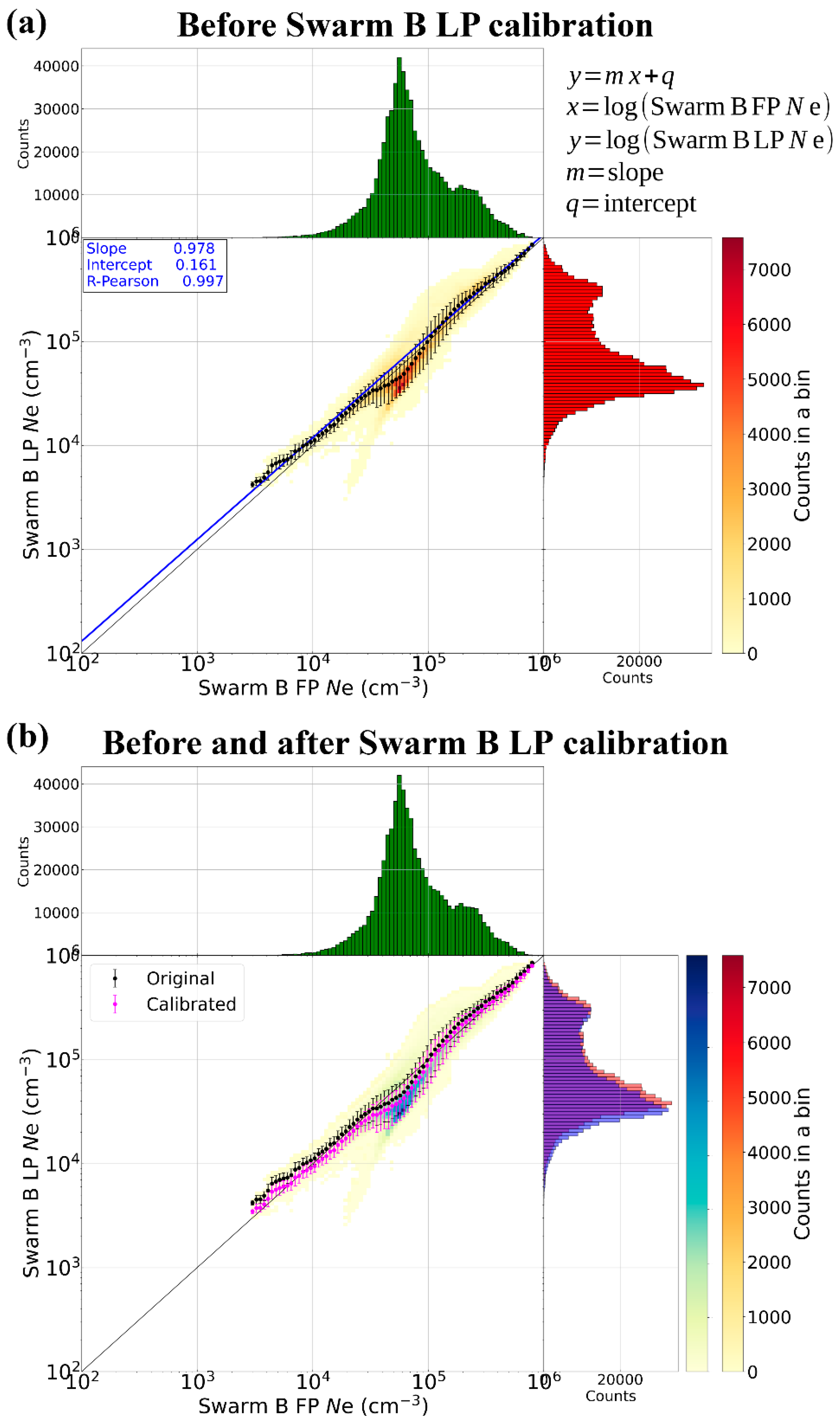
3.1. Calibration of Swarm B LP Electron Density Observations through FP Observations

Based on the results provided by Smirnov et al. [3] and Xiong et al. [6], we developed a calibration procedure to correct Swarm B LP Ne observations by using the FP instrument data made from the same satellite. Since our final goal is the comparison with CSES-01 and following calibration through Swarm B data, we focused on the dataset described at the end of Section 2.2. This dataset encompasses only low solar activity levels, and this is why we did not sort data as a function of the solar activity. According to Xiong et al. [6], for low solar activity, Swarm LP nighttime observations heavily overestimate FP ones, while during daytime, a slight underestimation is present. FP observations were decimated to 2 Hz for a one-to-one comparison with LP observations. As explained in Section 2.2, FP data are not continuous in time; moreover, the availability of data for the years 2019−2021 is quite sparse. These FP data limitations did not allow uniformly sampling different months and properly describing the seasonal variations of observations. This is why we did not sort data as a function of the season.

The calibration procedure was performed on a statistical basis through joint probability distributions (JPDs) between LP and FP datasets. Specifically, values from FP were sorted on a logarithmic scale from 10² to 10⁶ cm⁻³, with 30 bins for each order of magnitude; the same was done for the LP corresponding values. Then, for each bin of FP values, we calculated the mean and standard deviation of LP values conditioned by FP (i.e., those LP values falling inside a specific FP bin). Panel (a) of Figure 1 reports the JPD between Swarm B LP observations (on y-axis) and corresponding values from FP (on x-axis) for the daytime sector; the scale of reds represents the number of pairs falling inside each bin of the JPD. The mean and standard deviation values of Swarm B LP observations conditioned by FP observations are represented as black dots and error bars, respectively. The calibration procedure is performed on the base of these mean values considering only values greater than 10³ cm⁻³. Values below 10³ cm⁻³, which are recorded only in the nighttime sector (see Figure 2), are very few and much scattered, making corresponding bins undersampled and statistically unreliable. The linearity between the two datasets suggests the implementation of a simple linear calibration in a log-log scale (logarithm in base 10):

$${\left\{\begin{array}{l}y=mx+q\\ x=\log \left(\mathrm{Swarm}\mathrm{B}\mathrm{FP}N\mathrm{e}\right)\\ y=\log \left(\mathrm{Swarm}\mathrm{B}\mathrm{LP}N\mathrm{e}\right)\end{array}\right.}_{,}$$

(1)

with m the slope and q the intercept of the linear relation.

The blue line in the Panel (a) of Figure 1 is the result of the application of Equation (1) to the mean values of Swarm B LP observations conditioned by FP ones, with coefficients given in the legend. We also provide the Pearson correlation coefficient (R-Pearson) describing the linear correlation between the two distributions. In this case, the R-Pearson value is very close to one, which legitimizes the use of Equation (1). Panel (a) of Figure 2 provides the results for the nighttime sector. JPDs and linear fitting coefficient values confirm the findings by Xiong et al. [6] for low solar activity. Indeed, in the daytime sector, the two datasets agree very well, with an overall slight underestimation by LP data and maximum negative departures in the range 10^4.3–10⁵ cm⁻³. Conversely, in the nighttime sector, most of the LP data overestimate FP ones; the higher the Ne, the higher the overestimation.

The inversion of the linear relation of Equation (1), with coefficients given by the linear fit, allows obtaining the correction of Swarm B LP observations:

$$\widehat{y}={10}^{\frac{y-q}{m}},$$

(2)

with $\widehat{y}=\mathrm{calibrated}\mathrm{Swarm}\mathrm{B}\mathrm{LP}N\mathrm{e}$.

To test the efficacy of the linear calibration procedure, in Panels (b) of Figure 1 and Figure 2, we overplot the JPDs obtained with $\widehat{y}$ values to those of Panels (a) in a scale of blues, and calculate the mean and standard deviation values of calibrated Swarm B LP observations conditioned by Swarm B FP ones, represented as magenta dots and error bars. The calibration procedure allows compensating for the original overestimation during nighttime; while, during daytime, the differences are small, as expected. The agreement between the two datasets is evidenced by the distributions of calibrated values spreading along the first-third quadrant bisector (thin black lines in Figure 1 and Figure 2). The most significant departures from linearity are present only at the low tail of the nighttime distributions (see Figure 2). In the next section, Swarm B LP observations corrected through FP observations will be used as reference to calibrate CSES-01 LP observations. After that, the correctness of such procedure will be assessed through comparison with ISRs observations.

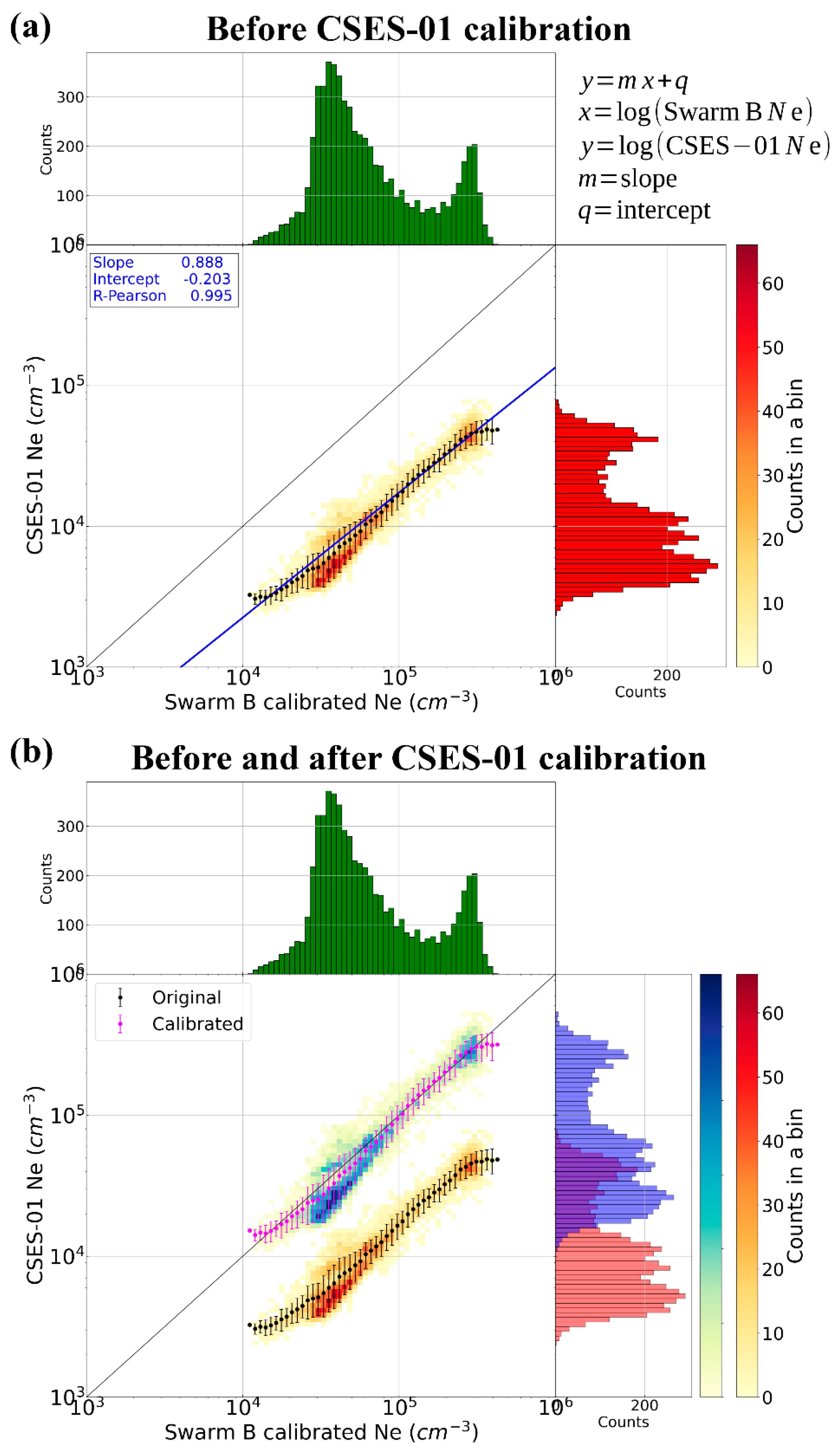
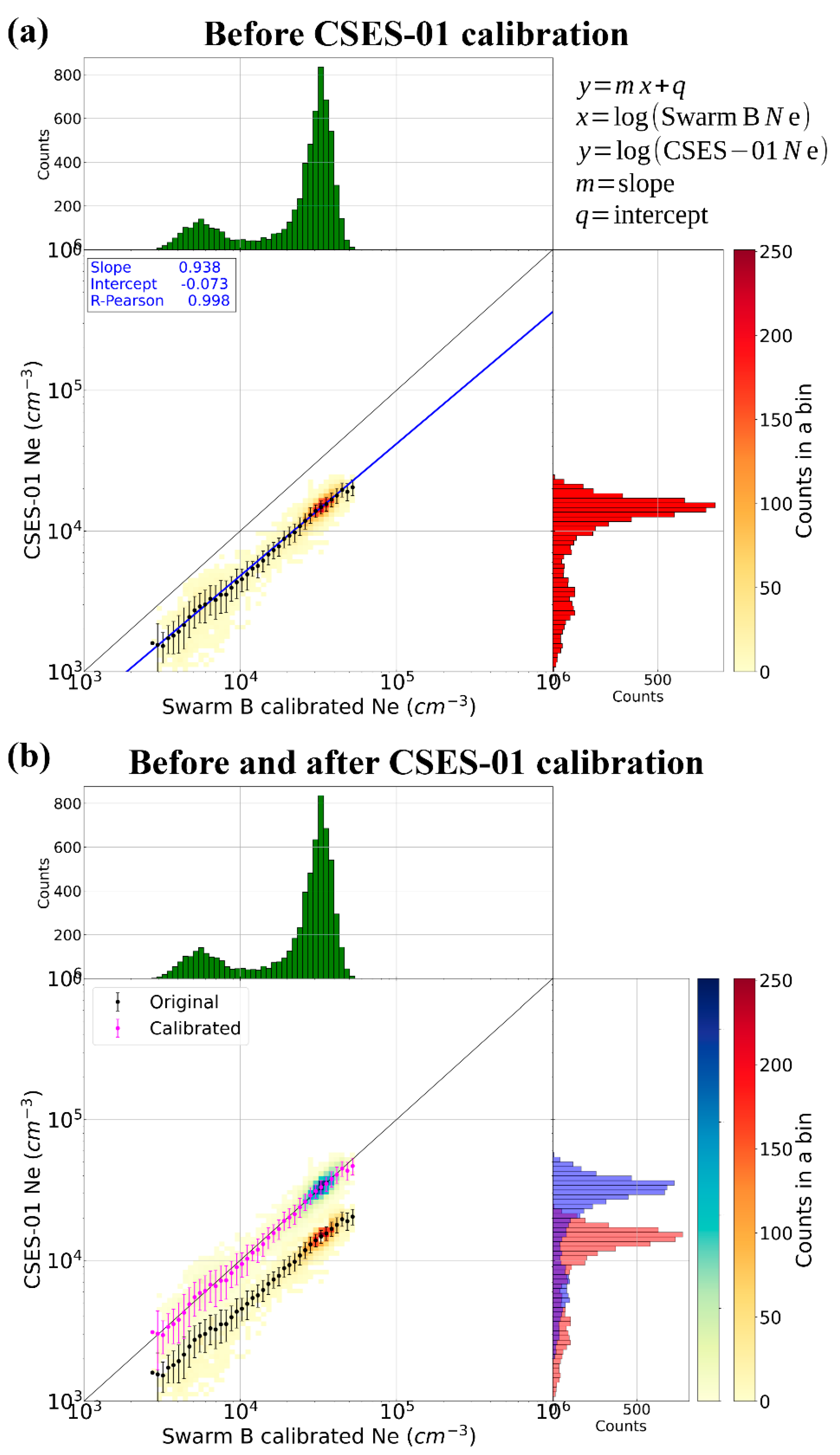
3.2. Calibration of CSES-01 Electron Density Observations through Swarm B Calibrated Electron Density Observations

Since CSES-01 and Swarm B satellites cover different locations at the same time, the application of a point-by-point calibration through the procedure described in Section 3.1 is not possible. It would have been possible only with a dataset of the satellites’ conjunctions. However, the number of such conjunctions is very small, and the corresponding dataset would have been biased towards the specific geophysical conditions of the days of the conjunctions. For these reasons, the calibration of CSES-01 LP Ne observations was performed on a statistical basis by considering the mean Ne values after sorting data as a function of geographic location and LT sector. Specifically, we sorted data according to the following criteria [28]:

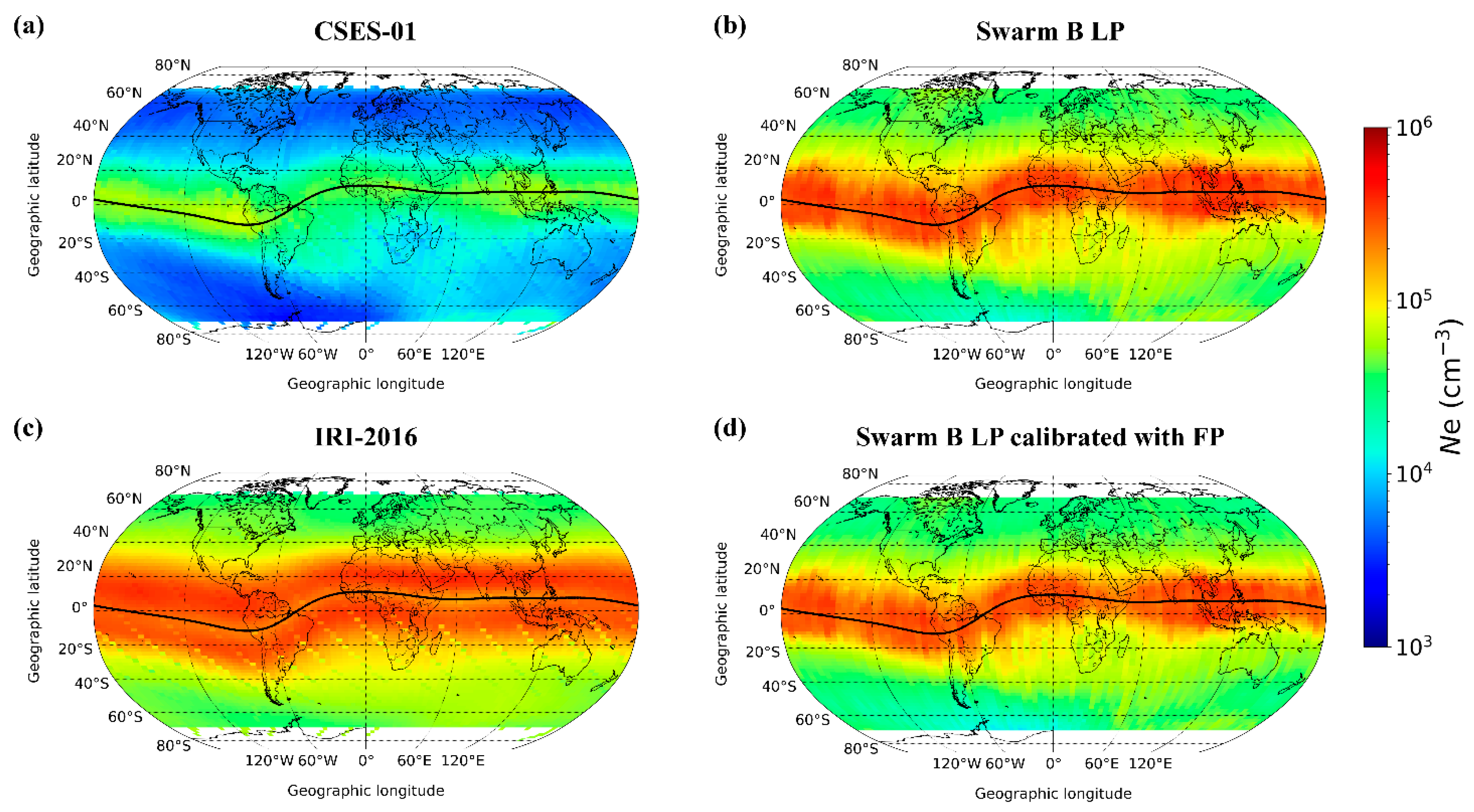
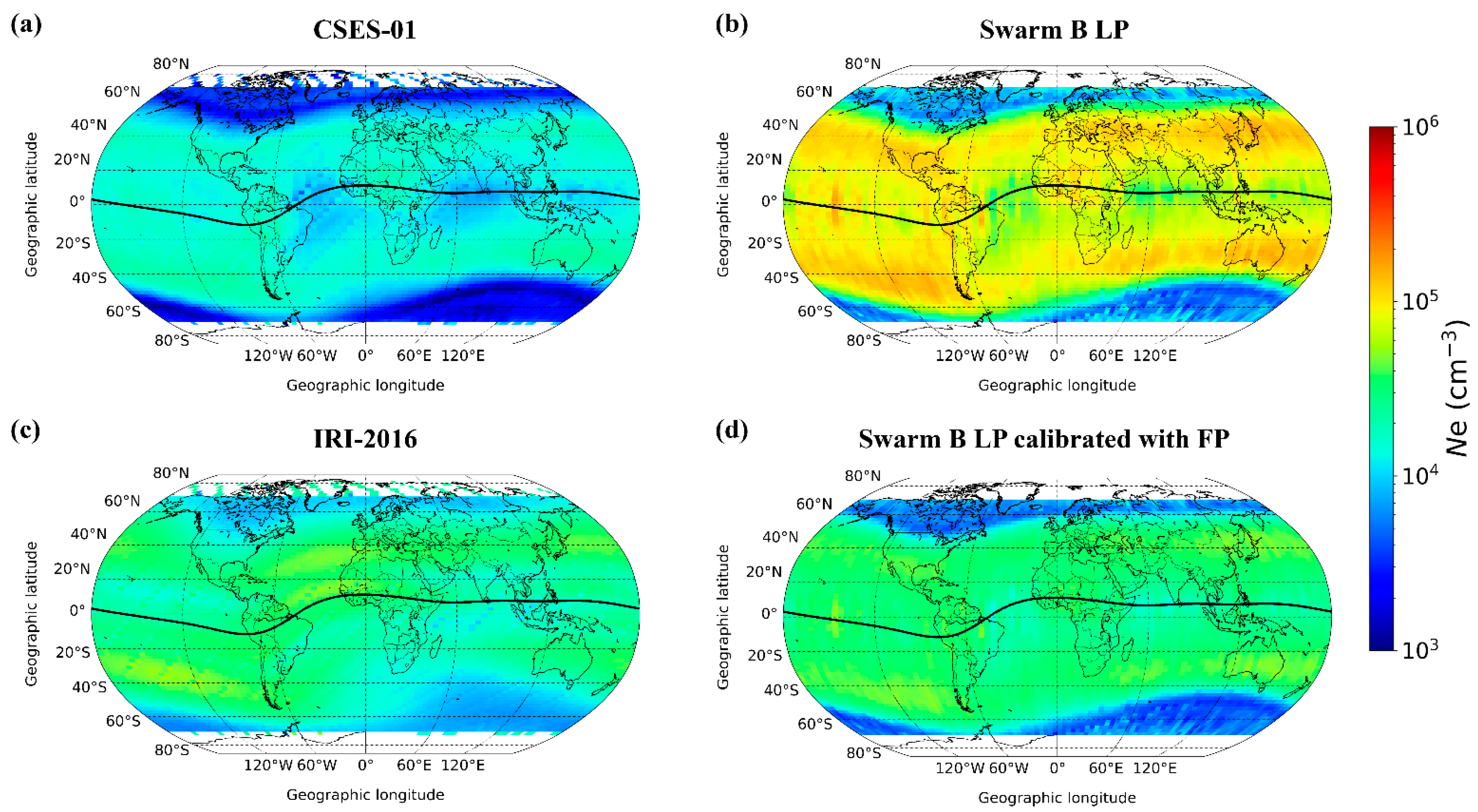
• Diurnal variation: data were sorted in two bins as a consequence of the CSES-01 orbit configuration, namely a nighttime sector representative of 02:00 LT and a daytime sector representative of 14:00 LT;
• Spatial geographic variation: for each diurnal bin, data were binned as a function of the geographic latitude and longitude. Specifically, data in the range 70°S–70°N were binned in bins 2°-wide in latitude and 4°-wide in longitude. Then, there are 6300 spatial bins for each diurnal sector.

For each bin, we calculated the mean value of Ne and represented such values as geographic maps. As explained before, a reliable statistical characterization of the seasonal dependence was not possible due to the limited extension of the available datasets. In addition, data were not sorted as a function of the solar activity level because our dataset encompasses only low solar activity levels.

Figure 3 and Figure 4 show, respectively, daytime and nighttime maps of Ne mean values as obtained by CSES-01, Swarm B LP, and Swarm B LP calibrated with FP and as modelled by IRI. Figure 3 highlights how much CSES-01 daytime values are smaller in magnitude than Swarm B and IRI ones, as already evidenced by several works in the literature [7,10,11]. Concerning the spatial variations, both measured and modelled values show maxima in a region surrounding the geomagnetic equator (represented by a black solid curve in the figure). However, while CSES-01 and Swarm B values show a single broad maximum centered at the geomagnetic equator, IRI predicts double maxima located at the equatorial ionization anomaly regions (at around ±15° of geomagnetic latitude) and a relative minimum at the geomagnetic equator. This is a well-known feature of IRI that is related to the topside ionosphere modelling made by the NeQuick option [23,29]. The comparison with data from several satellite missions highlighted this inconsistency related to the topside modelling made by IRI (e.g., [30]). In order to improve this IRI shortcoming, CSES-01 observations, along with those from other satellite missions, play a key role, as demonstrated by the good agreement among CSES-01 and other satellites related to the Ne spatial patterns. However, the very large differences in magnitude between CSES-01 and IRI have to be carefully investigated. As expected by looking at the results of Section 3.1, in the daytime sector the application of the calibration of Swarm B LP observations through FP ones produces a marginal effect. At the same time, it is worth noting how much Swarm B observations agree in magnitude with IRI ones during daytime. A completely different scenario opens up when considering nighttime observations.

Figure 4 evidences how nighttime Swarm B LP observations overestimate IRI ones in a large range of latitudes in both the Northern and Southern Hemispheres. The application of the calibration procedure based on FP observations corrects this overestimation by putting Swarm B observations in good agreement with IRI ones. Differently, CSES-01 underestimates IRI although to a lesser extent when compared to the daytime conditions. Again, concerning the spatial patterns, the good agreement between CSES-01 and Swarm B is remarkable.

The mean Ne values shown in Figure 3 and Figure 4 are used to statistically compare the CSES-01 LP and Swarm B LP calibrated datasets through the statistical procedure based on JPDs outlined in Section 3.1 for both LT sectors. In this case, JPDs are based on the 6300 binned Ne mean values (70 bins in latitude times 90 bins in longitude) from Figure 3 and Figure 4 maps.

Panel (a) of Figure 5 shows the comparison between CSES-01 LP mean values (on y-axis) and corresponding calibrated values from Swarm B LP (on x-axis) for the daytime sector. Corresponding results for the nighttime sector are shown in Panel (a) of Figure 6. The layout of Figure 5 and Figure 6 is the same as Figure 1 and Figure 2. JPDs confirm the striking linear correlation between CSES-01 and Swarm B. Further, the underestimation made by CSES-01 stands out for both conditions; on the other hand, the very good linear relation between the two datasets allows performing a linear calibration such as that done in Section 3.1. Then, the linear relation of Equation (1) is fitted to the mean values of CSES-01 values conditioned by calibrated Swarm B LP ones. In this case, $x=\log \left(\mathrm{Swarm}\mathrm{B}\mathrm{LP}N\mathrm{e}\mathrm{calibrated}\right)$ and $y=\log \left(\mathrm{CSES}\text{-}01N\mathrm{e}\right)$. The blue line in Panel (a) of Figure 5 and Figure 6 represents the linear fitting, and corresponding coefficients are given in the legend. The retrieved R-Pearson values very close to one confirm the linear relation between the two datasets and legitimize the application of the linear calibration procedure. The extent of the CSES-01 underestimation is provided by intercept coefficients, which are more pronounced during daytime (q = −0.203) than during nighttime (q = −0.073).

The application of Equation (2) with coefficients given by the linear fitting of Figure 5 and Figure 6 allows calibrating CSES-01 LP observations and obtaining $\widehat{y}=\mathrm{calibrated}\mathrm{CSES}\text{-}01\mathrm{LP}N\mathrm{e}$. The comparison between original and calibrated CSES-01 LP JPDs (Panel (b) of Figure 5 and Figure 6) highlights how the calibration procedure allows compensating the original underestimation without affecting the linear trend. Moreover, the goodness of the procedure is testified by the distributions spreading along the first-third quadrant bisector (thin black lines in Figure 5 and Figure 6) for the entire range of values.

Maps of calibrated CSES-01 LP Ne values are represented in the Panels (b) and (d) of Figure 7. The comparison with calibrated Swarm B LP Ne in Panels (a) and (c) of Figure 7, and with maps in Figure 3 and Figure 4 points out how the application of the calibration procedure is effective in correcting the magnitude of CSES-01 values. To evaluate the extent of the magnitude correction, the relative residuals between CSES-01 and Swarm B maps were calculated before and after CSES-01 data calibration. Specifically, percentage relative residuals (PRR) are calculated as:

$$\mathrm{PRR}[\%]=\frac{(\mathrm{CSES}\text{-}01N\mathrm{e})-(\mathrm{Swarm}\mathrm{B}N\mathrm{e})}{\mathrm{Swarm}\mathrm{B}N\mathrm{e}}\cdot 100.$$

(3)

In Equation (3), Swarm B values are the ones calibrated with FP (Panels (a) and (c)) of Figure 7). Instead, for CSES-01 values, for comparison purposes, we alternatively used the original ones (Panel (a) of Figure 3 and Figure 4) and the calibrated ones (Panels (b) and (d) of Figure 7). Results are shown in Figure 8.

Maps on the left (Panels (a) and (c)) show PRR values between original CSES-01 values and Swarm B LP values calibrated with FP. During daytime, the mean PRR is −83.0%, while during nighttime, it is −54.6%, thus confirming the well-known CSES-01 underestimation. Maps on the right (Panels (b) and (d)) show PRR values after the calibration of CSES-01 values. In this case, we have mean PRR values equal to −6.9% and −0.9% during daytime and nighttime, respectively, which confirms the efficacy of the calibration procedure. At the same time, these maps highlight more clearly the spatial regions where CSES-01 and Swarm B observations differ the most. In fact, even though the mean PRR values, calculated over the entire maps, are close to zero, there are regions where CSES-01 statistically overestimates Swarm B (in red) and regions where an underestimation prevails (in blue). It is of relevance to note that the locations where this happens are not random but exhibit a quite clear pattern, which also depends on the LT sector. This is because the calibration procedure applied in this section does not explicitly consider spatial variations, which means that spatial differences between the two datasets are not levelled by the calibration procedure. Systematic differences between the two datasets that were hidden before applying the calibration procedure are consequently highlighted.

3.3. Validation through Incoherent Scatter Radars Observations

The reliability and efficacy of the calibration procedure described in the previous sections needs to be tested against independent observations. In this regard, Ne observations by ISRs are considered the ground-truth to rely on for validation of in situ LP observations [4,5,6,31,32].

Since ISRs observations are not continuous in time and are performed only for a few days per month, we collected all the available ISRs observations at Jicamarca, Arecibo, and Millstone Hill (see Section 2.4) and performed a climatological statistical analysis similarly to Pignalberi et al. [26]. Specifically, for each of the three ISRs, we sorted data in the range of altitude 510 ± 20 km as a function of LT, in bins 30 min wide, to highlight the diurnal trends. To be consistent with the previous analyses, the seasonal variation was not considered, and only observations recorded in the range F10.7₈₁ < 90 sfu, which is representative of low solar activity level of the years 2019–2021, were considered. For each bin, we calculated the following statistical metrics:

• Counts in the bin;
• Median, i.e., the 50th percentile;
• First (25th percentile) and third (75th percentile) quartiles representative of the inter-quartile range (IQR);
• 5th and 95th percentiles, highlighting the tails of the distribution.

These statistical metrics are represented as boxplots and histograms in Figure 9 for Jicamarca, Arecibo, and Millstone Hill.

To make a comparison with ISRs data, we selected all the CSES-01 observations collected around the ISRs over an area centered at ISRs’ geographic location and extending ±5° in latitude and ±20° in longitude. Then, the selected CSES-01 observations were binned for the two LT sectors probed by CSES-01, and the corresponding median values are plotted. In Figure 9, the magenta star is the median of CSES-01 original values, while the green star is the median of CSES-01 calibrated values. For comparison purposes, the Swarm B FP observations collected over the ISRs and corresponding values modelled by IRI along the Swarm B orbit were also considered. The spatial selection criteria of both Swarm B FP and IRI values are exactly the same as CSES-01. However, due to the orbital configuration of Swarm B, all the LTs were covered, and the entire diurnal trend is represented.

The most striking features from Figure 9 are:

(a)

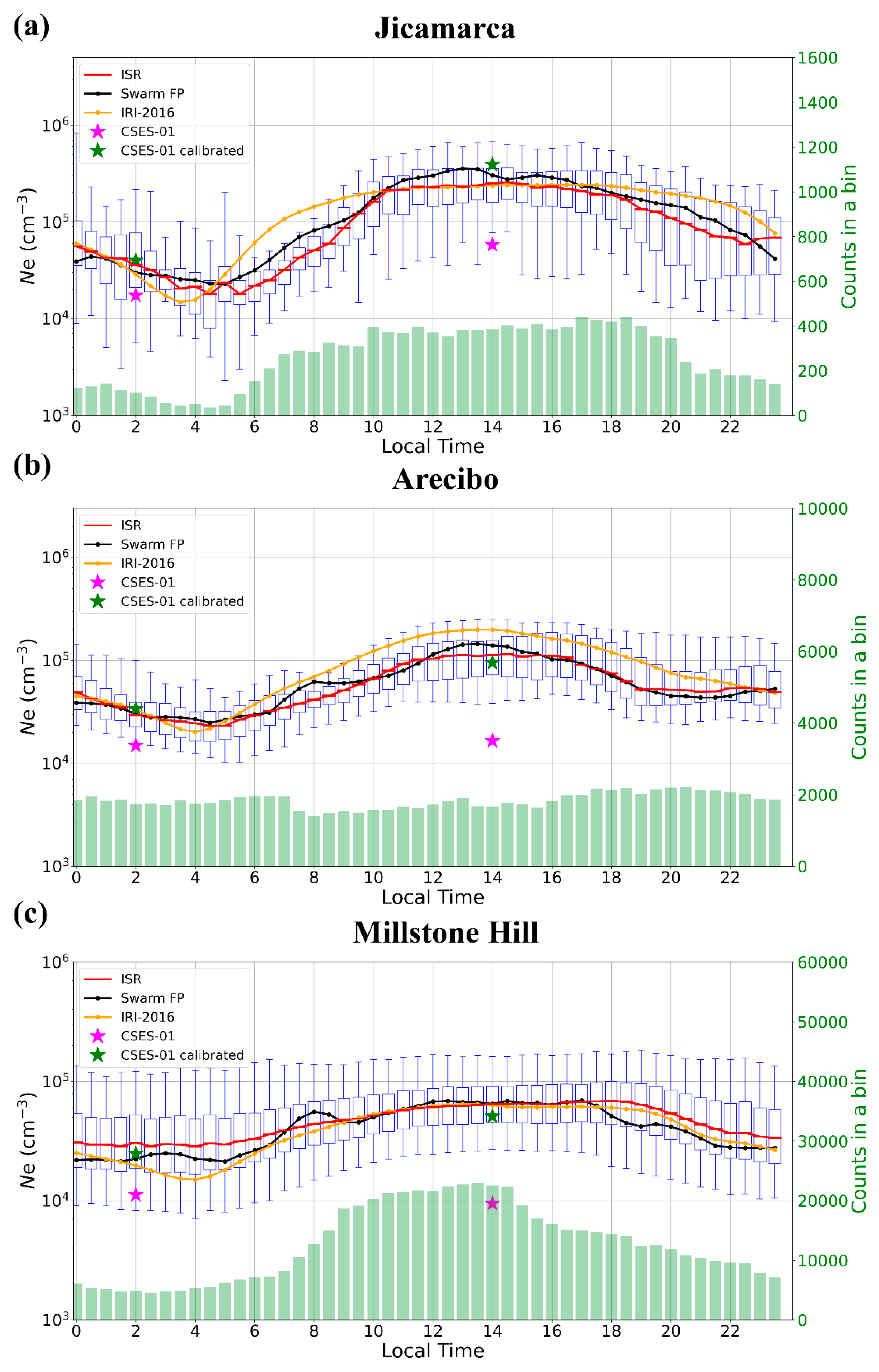
Original CSES-01 LP observations underestimate ISRs observations for both daytime and nighttime sectors for all the three locations. The application of the calibration procedure based on Swarm B LP observations calibrated with FP data strongly reduces this underestimation by bringing CSES-01 observations into agreement with ISRs ones within the IQR. Focusing on daytime values, after applying the calibration, CSES-01 slightly overestimates ISR values at Jicamarca, while a slight underestimation is visible both at Arecibo and Millstone Hill. This agrees with the PRR spatial patterns shown in Panel (b) of Figure 8. After applying the calibration, the nighttime results are very consistent, as was already evidenced by Panel (d) of Figure 8;

(b)

Swarm B FP observations are very accurate both in terms of magnitude and LT pattern, with values within the IQR, for all the three ISRs. This analysis testifies the goodness and reliability of Swarm FP observations, at least for the low solar activity level conditions investigated here. Compared to Swarm B LP observations (not shown in Figure 9), FP observations are by far more accurate in the description of nighttime conditions, as has been recently highlighted by Xiong et al. [6]. Most of the differences between Swarm B FP and ISRs are limited to the morning hours at Jicamarca (slight overestimation) and to nighttime conditions at Millstone Hill (slight underestimation);

(c)

The IRI topside model of Ne is statistically very reliable during daytime at mid latitudes (see Panel (c) for Millstone Hill). This is an expected behavior because IRI is an empirical model whose underlying dataset is heavily biased towards mid latitudes, where most of the ionospheric stations and facilities are located. A slightly degraded performance is visible during daytime around the equatorial ionization anomaly (see Panel (b) for Arecibo) and concerning the early morning trend at equatorial latitudes (see Panel (a) for Jicamarca). Anyway, in most cases, the IRI model reliably describes the Ne variations at CSES-01 altitude for the considered ISRs locations, making it a very robust benchmark for satellite in situ observations comparisons.

Finally, the statistical comparison with ISRs observations highlights the effectiveness of the proposed calibration procedure applied to CSES-01 LP data in reducing the underestimation suffered by CSES-01 observations during both daytime and nighttime.

4. Discussion

From our comparisons, it is clear that CSES-01 LP Ne data present an underestimation problem. In general, this could be due to several issues, spanning from an instrumental malfunction to estimation method systematic errors. We excluded all possible instrumental issues since the I–V characteristic curves produced by the CSES-01 LP are clear and smooth (see Yan et al. [13] for more details). We investigated any possible problem related to the inversion algorithm used for the evaluation of both Ne and Te. It is well-known that, on the basis of the orbital-motion-limited (OML) theory [33], once the electron current incident on the probe is at zero potential with respect to the surrounding plasma is known, Ne is linearly dependent on the inverse of the square root of Te. Thus, any possible systematic error in the evaluation of Te will produce an error in the Ne value. In our case, with Ne being underestimated, one possible explanation might be an overestimation of Te. Van Rompuy et al. [34] showed that a spherical LP can produce an overestimation of Te in presence of a non-Maxwellian electron velocity distribution, such as in the presence of two ion species plasma population. In fact, in such a condition, the general equation relating the electron current to Ne is no longer valid [33], being based on the assumption that electrons follow a Maxwellian distribution of velocities [35], and this needs to be evaluated integrating the correct electron distribution function. Hoegy and Brace [36] showed that additional electron population can be produced in the ionosphere by: (1) photoelectrons produced in the daytime ionosphere; (2) degraded secondary electrons produced by precipitating particles in the auroral oval; (3) photoelectrons produced by sunlit spacecraft surfaces; (4) secondary electrons produced by the impact at spacecraft velocities of thermospheric molecules; (5) secondary electrons emitted when the spacecraft potential is high enough to accelerate ionospheric ions or electrons to energies that exceed the ionization potential of spacecraft metallic surfaces; and (6) electron beams or plumes emitted from devices onboard the satellite. In general, (1) and (2) have a negligible influence on the I–V curves and can be neglected. On the other hand, (3)–(6) can have high enough densities to significantly distort the I–V curves and affect the determination of Te by distorting the electron retarding regions [37,38,39]. The calibration procedure applied here cannot give indications of what the main physical causes of CSES-01 LP Ne underestimation are. However, the evidences brought by our analyses and by the considerations described above point toward the need of a careful analysis of CSES-01 LP Te observations. Moreover, the possible inclusion of non-Maxwellian electron velocity distribution in the inversion algorithm used for the evaluation of both Ne and Te is a point to be investigated in a forthcoming analysis.

One aspect that deserves to be discussed in more detail concerns the calibration of Swarm LP data by using FP measurements. The Swarm LPs operating mode is rather different than the CSES-01 LP’s one: instead of continuously sweeping an applied voltage and collecting the current, which is the standard method to operate a LP, three fixed voltages on an ideal I–V curve are determined, and a periodic ripple is superposed to each of the applied voltages for a duration of about 100 ms. This allows determining not only the collected current but also the complex admittance, which is the derivative of the ideal I–V curve in the selected point. By combining currents and admittances measurements in the framework of the OML theory, Ne, Te, and the spacecraft potential can be inferred (full details can be found in Knudsen et al. [19]). Since the so-called “ion region” of the ideal I–V curve, where a negative voltage is applied, is less disturbed than the “electron region”, in the Swarm LP processing, Ne is obtained from the ion region. As a consequence, what Swarm LPs measure is the ion density, Ni, rather than Ne; however, this does not represent a problem since quasi-neutrality (Ne ≅ Ni) holds for ionospheric plasma. Nevertheless, in the framework of the Swarm LP processing, two major assumptions are needed: (1) the only ion species present at these heights is O⁺; (2) the along-track ion speed is always negligible with respect to the satellite speed. These are reasonable assumptions most of the time but, as pointed out by Pakhotin et al. [32], a non-negligible fraction of H⁺ ions can be present, especially during the night and at Swarm B heights (e.g., [3,6]): even a small fraction of ions lighter than O⁺ can considerably reduce the effective mass that enters in the ion density determination so that neglecting this contribution could lead to an overestimation of density. On the other hand, FP measurements do not imply any a priori assumption on the ion species detected although still, as for the LPs, the along-track ion speed is neglected. Overall, the picture is consistent with results: as seen in Figure 2, the nighttime portion of Swarm B LP dataset overestimates the corresponding FP one. Instead, the Swarm B LP dataset calibrated with the Swarm B FP dataset can safely be compared with a “true” Ne dataset such as that from CSES-01 LP. A word of caution should nevertheless be brought considering that such cross-validation between Swarm B and CSES-01 datasets is limited to the time period taken into account, mainly characterized by low solar activity; while, for high and intense solar activity periods, the results could be very different [6]. As a consequence, to confirm the goodness of FP data and the effectiveness of the calibration procedure applied to LP data, the procedure described in Section 3.1 should be repeated for higher solar activity levels, which is possible because simultaneous LP and FP observations are available from October 2014 onwards, thus embracing the second part of the last solar cycle. Moreover, it has to be proven that this calibration procedure could be also applied for LTs different from those studied in this work and, if so, to study the LT behavior of calculated calibration parameters. Both these issues are beyond the scope of this paper but deserve attention for the future improvement of the Swarm LP dataset.

The calibration procedure applied to CSES-01 LP Ne data allowed improving the agreement with corresponding ISRs Ne data for the two LT sectors probed by CSES-01 (see Figure 9) and with both Swarm B LP calibrated data and IRI-modelled data (see Figure 3, Figure 4, Figure 7 and Figure 8). This study represents a preliminary but fundamental step towards the use of CSES-01 LP Ne data for topside ionosphere modelling and improvement of empirical models such as IRI [1] and NeQuick [23]. Indeed, despite the reliable representation of the Ne spatial and LT variations in the topside ionosphere provided by CSES-01 LP observations, the remarkable underestimation evidenced by previous studies [7,10,11] prevented from using CSES-01 LP Ne data for empirical modelling of the topside ionosphere. The application of our calibration procedure fixes this issue and opens up the way to several applications. For instance, CSES-01 LP Ne observations can be used to calculate the topside plasma effective scale height with the procedure implemented by Pignalberi et al. [40] and later applied to the NeQuick model by Pezzopane and Pignalberi [41], both making use of Swarm satellites LP Ne data. Since the topside plasma effective scale height is the parameter driving the decay of Ne in the topside ionosphere, thus controlling the shape of the topside vertical Ne profile [42], a reliable specification of this parameter is fundamental for empirical models and to retrieve reliable vertical total electron content values. Moreover, Pignalberi et al. [43] also demonstrated that such effective scale height is linked to the vertical scale height theoretically deduced from the plasma ambipolar diffusion theory so that, from the study of its variations, some physical properties of the plasma in the topside ionosphere can be inferred. CSES-01 LP Ne data can be profitably used to fix the IRI representation of the low-latitude topside ionosphere at LEO altitudes in the daytime sector. In fact, IRI at these altitudes predicts the presence of a double maximum located at the equatorial ionization anomaly regions, while CSES-01 (in agreement with Swarm B and other satellite missions) shows a single broad maximum centered at the geomagnetic equator. The inclusion of CSES-01 LP Ne calibrated data in the dataset underlying IRI would help to solve this issue, as recently demonstrated by Bilitza and Xiong [29], who made use of CHAMP, GRACE, and Swarm satellites data to improve the IRI topside model.

5. Conclusions

To fix the underestimation characterizing the CSES-01 LP Ne observations, we developed a calibration procedure taking advantage of LP and FP observations recorded by Swarm B satellite flying at an altitude similar to that of CSES-01 (about 500 km above the ground). As a preliminary step, Swarm B LP data were calibrated through the FP dataset, which shows a better agreement with ISRs measurements made at Jicamarca, Arecibo, and Millstone Hill. This calibration allowed solving the Swarm B LP overestimation during nighttime hours and for low solar activity, evidenced by Smirnov et al. [3] and Xiong et al. [6]. Calibrated Swarm B LP observations were then used to calibrate corresponding CSES-01 LP values. Overall, the calibration procedure resulted in strongly reducing the CSES-01 LP underestimation. When compared to calibrated Swarm LP data, the mean PRR was reduced from −83.0% to −6.9% during daytime and from −54.6% to −0.9% during nighttime. The effectiveness of the calibration procedure was, finally, statistically assessed against independent measurements from Jicamarca, Arecibo, and Millstone Hill ISRs. After the calibration, CSES-01 LP data were in agreement with ISRs ones within the IQR, contrary to the original data, which were highly underestimated. The improvement brought by the calibration was verified for both daytime and nighttime sectors and for the different latitudes of the ISRs locations. Calibrated CSES-01 LP data were also in agreement with IRI modelled data.

Since the calibration procedure proposed here is based on data recorded from 1 January 2019 to 30 September 2021, it encompasses only low solar activity conditions. As a consequence, when new data from both CSES-01 and Swarm B satellites will be available in the next years, the possible dependence of the calibration coefficients on solar activity will be investigated. Moreover, due to the shortness of the available dataset, this work did not investigate a possible seasonal dependence of calibration coefficients. This is another point that will be considered in the future when more data will be available. Furthermore, the calibration procedure was applied on data recorded at different latitudes; however, PRR maps of Figure 8 highlight latitudinal differences between calibrated CSES-01 and Swarm B data, particularly during daytime. Since our main goal is to smooth the large CSES-01 Ne underestimation and provide the ionospheric community a simple methodology to correct CSES-01 Ne data, at this stage, the latitudinal dependence was not considered in the calibration procedure. Further studies based on a more extended dataset are needed to also take into consideration this dependence as well as those on seasons and solar activity.

CSES-01 is the first of a series of Chinese LEO satellites dedicated to geophysical measurements and near-Earth environment monitoring. Other satellites will be launched in the coming years, covering different LTs and thus also allowing a complete description of the diurnal behavior of the topside ionosphere. Since the satellites to be launched will carry a Langmuir probe on board, the results of this study can be of value for future CSES missions to foster the use of CSES observations for ionospheric modelling.

Last but not least, CSES-01 LP Ne observations calibrated through the procedure described in this paper can be profitably used for empirical modelling of the topside ionosphere and for the improvement of models such as IRI and NeQuick.

References

1. Bilitza, D.; Altadill, D.; Truhlik, V.; Shubin, V.; Galkin, I.; Reinisch, B.; Huang, X. International reference ionosphere 2016: From ionospheric climate to real-time weather predictions. Space Weather 2017, 15, 418–429. [Google Scholar] [CrossRef]
2. Shen, X.H.; Zhang, X.M.; Yuan, S.G.; Wang, L.W.; Cao, J.B.; Huang, J.P.; Zhu, X.H.; Picozza, P.; Dai, J.P. The state-of-the-art of the China Seismo-Electromagnetic Satellite mission. Sci. China Technol. Sci. 2018, 61, 634–642. [Google Scholar] [CrossRef]
3. Smirnov, A.; Shprits, Y.; Zhelavskaya, I.; Lühr, H.; Xiong, C.; Goss, A.; Prol, F.S.; Schmidt, M.; Hoque, M.; Pedatella, N.; et al. Intercalibration of the plasma density measurements in Earth’s topside ionosphere. J. Geophys. Res. Space Phys. 2021, 126, e2021JA029334. [Google Scholar] [CrossRef]
4. Lomidze, L.; Knudsen, D.J.; Burchill, J.; Kouznetsov, A.; Buchert, S.C. Calibration and validation of Swarm plasma densities and electron temperatures using ground-based radars and satellite radio occultation measurements. Radio Sci. 2018, 53, 15–36. [Google Scholar] [CrossRef]
5. Larson, B.; Koustov, A.V.; Kouznetsov, A.F.; Lomidze, L.; Gillies, R.G.; Reimer, A.S. A comparison of the topside electron density measured by the Swarm satellites and incoherent scatter radars over Resolute Bay, Canada. Radio Sci. 2021, 56, e2021RS007326. [Google Scholar] [CrossRef]
6. Xiong, C.; Jiang, H.; Yan, R.; Lühr, H.; Stolle, C.; Yin, F.; Smirnov, A.; Piersanti, M.; Liu, Y.; Wan, X.; et al. Solar flux influence on the in-situ plasma density at topside ionosphere measured by Swarm satellites. J. Geophys. Res. Space Phys. 2022, 127, e2022JA030275. [Google Scholar] [CrossRef]
7. Wang, X.; Cheng, W.; Yang, D.; Liu, D. Preliminary validation of in situ electron density measurements onboard CSES using observations from Swarm Satellites. Adv. Space Res. 2019, 64, 982–994. [Google Scholar] [CrossRef]
8. Chen, P.; Li, Q.; Yao, Y.; Yao, W. Study on the plasmaspheric Weddell Sea Anomaly based on COSMIC onboard GPS measurements. J. Atmos. Sol. Terr. Phys. 2019, 192, 104923. [Google Scholar] [CrossRef]
9. Yasyukevich, Y.V.; Yasyukevich, A.S.; Ratovsky, K.G.; Klimenko, M.V.; Klimenko, V.V.; Chirik, N.V. Winter anomaly in NmF2 and TEC: When and where it can occur. J. Space Weather Space Clim. 2018, 8, A45. [Google Scholar] [CrossRef]
10. Yan, R.; Zhima, Z.; Xiong, C.; Shen, X.; Huang, J.; Guan, Y.; Zhu, X.; Liu, C. Comparison of electron density and temperature from the CSES satellite with other space-borne and ground-based observations. J. Geophys. Res. Space Phys. 2020, 125, e2019JA027747. [Google Scholar] [CrossRef]
11. Liu, J.; Guan, Y.; Zhang, X.; Shen, X. The data comparison of electron density between CSES and DEMETER satellite, Swarm constellation and IRI model. Earth Space Sci. 2021, 8, e2020EA001475. [Google Scholar] [CrossRef]
12. Liu, C.; Guan, Y.; Zheng, X.; Zhang, A.; Piero, D.; Sun, Y. The technology of space plasma in-situ measurement on the China Seismo-Electromagnetic Satellite. Sci. China Technol. Sci. 2019, 62, 829–838. [Google Scholar] [CrossRef]
13. Yan, R.; Guan, Y.; Shen, X.; Huang, J.; Zhang, X.; Liu, C.; Liu, D. The Langmuir Probe onboard CSES: Data inversion analysis method and first results. Earth Plan. Phys. 2018, 2, 479–488. [Google Scholar] [CrossRef]
14. Langmuir, I.; Mott-Smith, H.M. Studies of electric discharges in gases at low pressures. Gen. Electr. Rev. 1924, 27, 449–455. [Google Scholar]
15. Langmuir, I. Electric discharges in gases at low pressures. J. Frankl. Inst. 1932, 214, 275–298. [Google Scholar] [CrossRef]
16. Mott-Smith, H.M. The theory of collectors in gaseous discharges. In Electrical Discharge; Suits, C.G., Ed.; Elsevier: Amsterdam, The Netherlands, 1961; pp. 99–132. [Google Scholar] [CrossRef]
17. Lebreton, J.-P.; Stverak, S.; Travnicek, P.; Maksimovic, M.; Klinge, D.; Merikallio, S.; Lagoutte, D.; Poirier, B.; Blelly, P.-L.; Kozacek, Z.; et al. The ISL Langmuir probe experiment processing onboard DEMETER: Scientific objectives, description and first results. Planet. Space Sci. 2006, 54, 472–486. [Google Scholar] [CrossRef]
18. Friis-Christensen, E.; Lühr, H.; Knudsen, D.; Haagmans, R. Swarm—An earth observation mission investigating geospace. Adv. Space Res. 2008, 41, 210–216. [Google Scholar] [CrossRef]
19. Knudsen, D.J.; Burchill, J.K.; Buchert, S.C.; Eriksson, A.I.; Gill, R.; Wahlund, J.; Åhlen, L.; Smith, M.; Moffat, B. Thermal ion imagers and Langmuir probes in the Swarm electric field instruments. J. Geophys. Res. Space Phys. 2017, 122, 2655–2673. [Google Scholar] [CrossRef]
20. Catapano, F.; Buchert, S.; Qamili, E.; Nilsson, T.; Bouffard, J.; Siemes, C.; Coco, I.; D’Amicis, R.; Tøffner-Clausen, L.; Trenchi, L.; et al. Swarm Langmuir probes’ data quality validation and future improvements. Geosci. Instrum. Methods Data Syst. 2022, 11, 149–162. [Google Scholar] [CrossRef]
21. Rush, C.M.; Fox, M.; Bilitza, D.; Davies, K.; McNamara, L.; Stewart, F.G.; PoKempner, M. Ionospheric mapping-an update of foF2 coefficients. Telecommun. J. 1989, 56, 179–182. [Google Scholar]
22. Shubin, V.N. Global median model of the F2-layer peak height based on ionospheric radio-occultation and ground based digisonde observations. Adv. Space Res. 2015, 56, 916–928. [Google Scholar] [CrossRef]
23. Nava, B.; Coïsson, P.; Radicella, S. A new version of the NeQuick ionosphere electron density model. J. Atmos. Solar-Terr. Phys. 2008, 70, 1856–1862. [Google Scholar] [CrossRef]
24. Evans, J. Theory and practice of ionosphere study by Thomson scatter radar. Proc. IEEE 1969, 57, 496–530. [Google Scholar] [CrossRef]
25. Pignalberi, A.; Aksonova, K.D.; Zhang, S.-R.; Truhlik, V.; Gurram, P.; Pavlou, C. Climatological study of the ion temperature in the ionosphere as recorded by Millstone Hill incoherent scatter radar and comparison with the IRI model. Adv. Space Res. 2021, 68, 2186–2203. [Google Scholar] [CrossRef]
26. Pignalberi, A.; Giannattasio, F.; Truhlik, V.; Coco, I.; Pezzopane, M.; Consolini, G.; De Michelis, P.; Tozzi, R. On the Electron Temperature in the Topside Ionosphere as Seen by Swarm Satellites, Incoherent Scatter Radars, and the International Reference Ionosphere Model. Remote Sens. 2021, 13, 4077. [Google Scholar] [CrossRef]
27. Tapping, K.F. The 10.7 cm solar radio flux (F10.7). Space Weather 2013, 11, 394–406. [Google Scholar] [CrossRef]
28. Pezzopane, M.; Pignalberi, A.; De Michelis, P.; Consolini, G.; Coco, I.; Giannattasio, F.; Tozzi, R.; Zoffoli, S. On the Best Settings to Calculate Ionospheric Irregularity Indices From the In Situ Plasma Parameters of CSES-01. IEEE J. Sel. Top. Appl. Earth Obs. Remote Sens. 2022, 15, 4058–4071. [Google Scholar] [CrossRef]
29. Bilitza, D.; Xiong, C. A solar activity correction term for the IRI topside electron density model. Adv. Space Res. 2021, 68, 2124–2137. [Google Scholar] [CrossRef]
30. Pignalberi, A.; Pezzopane, M.; Tozzi, R.; De Michelis, P.; Coco, I. Comparison between IRI and preliminary Swarm Langmuir probe measurements during the St. Patrick storm period. Earth Planets Space 2016, 68, 93. [Google Scholar] [CrossRef]
31. Xiong, C.; Lühr, H.; Ma, S.-Y.; Schlegel, K. Validation of GRACE electron densities by incoherent scatter radar data and estimation of plasma scale height in the topside ionosphere. Adv. Space Res. 2015, 55, 2048–2057. [Google Scholar] [CrossRef]
32. Pakhotin, I.P.; Burchill, J.K.; Förster, M.; Lomidze, L. The swarm Langmuir probe ion drift, density and effective mass (SLIDEM) product. Earth Planets Space 2022, 74, 109. [Google Scholar] [CrossRef]
33. Merlino, R.L. Understanding Langmuir probe current-voltage characteristics. Am. J. Phys. 2007, 75, 1078. [Google Scholar] [CrossRef]
34. Van Rompuy, T.; Gunn, J.P.; Dejarnac, R.; Stöckel, J.; Van Oost, G. Sensitivity of electron temperature measurements with the tunnel probe to a fast electron component. Plasma Phys. Control. Fusion 2007, 49, 619. [Google Scholar] [CrossRef]
35. Schott, L. Electric Probes in Plasma Diagnostics; Lochte-Holtgreven, W., Ed.; Elsevier: New York, NY, USA, 1968; Chapter 11. [Google Scholar]
36. Hoegy, W.R.; Brace, L.H. Use of Langmuir probes in non-Maxwellian space plasmas. Rev. Sci. Instrum. 1999, 70, 3015–3024. [Google Scholar] [CrossRef]
37. Whipple, E.C.; Brace, L.H.; Parker, L.W. Impact Ionization Effects on Pioneer Venus Orbiter. In Proceedings of the 17th ESLAB Symposium on Spacecraft Interactions, Noordwijk, The Netherlands, 13–16 September 1983; ESA Report SP-198. p. 127. [Google Scholar]
38. Brace, L.H.; Theis, R.F.; Mayr, H.G.; Curtis, S.A.; Luhmann, J.G. Holes in the nightside ionosphere of Venus. J. Geophys. Res. 1982, 87, 199. [Google Scholar] [CrossRef]
39. Knudsen, C.W.; Miller, K.L. Pioneer Venus suprathermal electron flux measurements in the Venus umbra. J. Geophys. Res. 1985, 90, 2695. [Google Scholar] [CrossRef]
40. Pignalberi, A.; Pezzopane, M.; Rizzi, R. Modeling the lower part of the topside ionospheric vertical electron density profile over the European region by means of Swarm satellites data and IRI UP method. Space Weather 2018, 16, 304–320. [Google Scholar] [CrossRef]
41. Pezzopane, M.; Pignalberi, A. The ESA Swarm mission to help ionospheric modeling: A new NeQuick topside formulation for mid-latitude regions. Sci. Rep. 2019, 9, 12253. [Google Scholar] [CrossRef]
42. Pignalberi, A.; Pezzopane, M.; Themens, D.R.; Haralambous, H.; Nava, B.; Coïsson, P. On the Analytical Description of the Topside Ionosphere by NeQuick: Modeling the Scale Height Through COSMIC/FORMOSAT-3 Selected Data. IEEE J. Sel. Top. Appl. Earth Obs. Remote Sens. 2020, 13, 1867–1878. [Google Scholar] [CrossRef]
43. Pignalberi, A.; Pezzopane, M.; Nava, B.; Coïsson, P. On the link between the topside ionospheric effective scale height and the plasma ambipolar diffusion, theory and preliminary results. Sci. Rep. 2020, 10, 17541. [Google Scholar] [CrossRef]
Figure 1. JPDs between Swarm B LP Ne observations (y-axis) and Swarm B FP Ne observations (x-axis), both recorded from 1 January 2019 to 30 September 2021 in the range of latitudes between 70°S and 70°N for the daytime sector (13:00−15:00 LT). Panel (a) refers to Swarm B LP observations before the calibration, while Panel (b) also shows the distribution of Swarm B LP observations after applying the calibration. In each panel, histograms of the counts are also reported: on the right and in red for Swarm B LP before the calibration, in blue for Swarm B LP after the calibration, and on the top and in green for Swarm B FP. The black dots refer to the mean values of original Swarm B LP Ne observations conditioned by Swarm B FP Ne observations, with the corresponding standard deviation as error bar. The magenta dots refer to the mean values of calibrated Swarm B LP Ne observations conditioned by Swarm B FP Ne observations, with the corresponding standard deviation as error bar. The blue line in Panel (a) is the linear fit on black dots, with coefficients given in the legend. The thin black line is the first-third quadrant bisector.
Remotesensing 14 04679 g001
Figure 2. JPDs between Swarm B LP Ne observations (y-axis) and Swarm B FP Ne observations (x-axis), both recorded from 1 January 2019 to 30 September 2021 in the range of latitudes between 70°S and 70°N for the nighttime sector (01:00−03:00 LT). Panel (a) refers to Swarm B LP observations before the calibration, while Panel (b) also shows the distribution of Swarm B LP observations after applying the calibration. In each panel, histograms of the counts are also reported: on the right and in red for Swarm B LP before the calibration, in blue for Swarm B LP after the calibration, and on the top and in green for Swarm B FP. The black dots refer to the mean values of original Swarm B LP Ne observations conditioned by Swarm B FP Ne observations, with the corresponding standard deviation as error bar. The magenta dots refer to the mean values of calibrated Swarm B LP Ne observations conditioned by Swarm B FP Ne observations, with the corresponding standard deviation as error bar. The blue line in Panel (a) is the linear fit on black dots, with coefficients given in the legend. The thin black line is the first-third quadrant bisector.
Remotesensing 14 04679 g002
Figure 3. Geographical maps of Ne mean values measured by CSES-01 LP (Panel (a)), Swarm B LP (Panel (b)), and Swarm B LP after applying the calibration with FP observations (Panel (d)) and modelled by IRI-2016 along CSES-01 orbits (Panel (c)) for the daytime sector (13:00−15:00 LT). The mean is calculated on data ranging between 1 January 2019 and 30 September 2021. The thick black curve in each plot represents the geomagnetic equator.
Remotesensing 14 04679 g003
Figure 4. Geographical maps of Ne mean values measured by CSES-01 LP (Panel (a)), Swarm B LP (Panel (b)), and Swarm B LP after applying the calibration with FP observations (Panel (d)) and modelled by IRI-2016 along CSES-01 orbits (Panel (c)) for the nighttime sector (01:00−03:00 LT). The mean is calculated on data ranging between 1 January 2019 and 30 September 2021. The thick black curve in each plot represents the geomagnetic equator.
Remotesensing 14 04679 g004
Figure 5. JPDs between CSES-01 LP Ne (y-axis) and Swarm B LP Ne calibrated with FP (x-axis) mean values represented in Figure 3 for the daytime sector (13:00−15:00 LT). Panel (a) refers to CSES-01 before the calibration, while Panel (b) also shows the distribution of CSES-01 after the calibration. In each panel, histograms of the counts are also reported: on the right and in red for CSES-01 LP before the calibration, in blue for CSES-01 LP after the calibration, and on the top and in green for Swarm B LP Ne calibrated with FP. The black dots refer to the mean values of original CSES-01 Ne conditioned by Swarm B LP Ne calibrated with FP, with the corresponding standard deviation as error bar. The magenta dots refer to the mean values of calibrated CSES-01 Ne conditioned by Swarm B LP Ne calibrated with FP, with the corresponding standard deviation as error bar. The blue line in Panel (a) is the linear fit performed on black dots, with corresponding coefficients given in the legend. The thin black line is the first-third quadrant bisector.
Remotesensing 14 04679 g005
Figure 6. JPDs between CSES-01 LP Ne (y-axis) and Swarm B LP Ne calibrated with FP (x-axis) mean values represented in Figure 4 for the nighttime sector (01:00−03:00 LT). Panel (a) refers to CSES-01 before the calibration, while Panel (b) also shows the distribution of CSES-01 after the calibration. In each panel, histograms of the counts are also reported: on the right and in red for CSES-01 LP before the calibration, in blue for CSES-01 LP after the calibration, and on the top and in green for Swarm B LP Ne calibrated with FP. The black dots refer to the mean values of original CSES-01 Ne conditioned by Swarm B LP Ne calibrated with FP, with the corresponding standard deviation as error bar. The magenta dots refer to the mean values of calibrated CSES-01 Ne conditioned by Swarm B LP Ne calibrated with FP, with the corresponding standard deviation as error bar. The blue line in Panel (a) is the linear fit performed on black dots, with corresponding coefficients given in the legend. The thin black line is the first-third quadrant bisector.
Remotesensing 14 04679 g006
Figure 7. Geographical maps of mean Ne values measured by Swarm B LP after the calibration with FP observations (Panels (a,c)) and geographical maps of mean Ne values measured by CSES-01 LP after applying the calibration procedure based on Swarm B data (Panels (b,d)). Panels (a,b) are for the daytime sector (13:00−15:00 LT); Panels (c,d) are for the nighttime sector (01:00−03:00 LT). The thick black curve in each plot represents the geomagnetic equator.
Remotesensing 14 04679 g007
Figure 8. Geographical maps of percentage relative residuals between mean values of CSES-01 Ne and Swarm B LP Ne calibrated with FP. Panels (a,c) are for CSES-01 original data; Panels (b,d) are for CSES-01 data calibrated through Swarm B data. Panels (a,b) refer to the daytime sector (13:00−15:00 LT); Panels (c,d) refer to the nighttime sector (01:00−03:00 LT). In green, the mean of the percentage relative residuals calculated for the whole map is reported. Data encompass the period from 1 January 2019 to 30 September 2021. The thick black curve in each plot represents the geomagnetic equator.
Remotesensing 14 04679 g008
Figure 9. Statistical comparison among Ne observations by ISRs at around 510 km of altitude (boxplots), Swarm B FP (black line), and CSES-01 LP (magenta star for original values, green star for calibrated values) and modelled by IRI-2016 (orange line). Panel (a) refers to Jicamarca, Panel (b) refers to Arecibo, and Panel (c) refers to Millstone Hill. Both measured and modelled data are binned as a function of LT (x-axis) in bins 30 min wide. ISRs data are represented as boxplots in which the red line is the median; the 25th and 75th percentiles are represented as the lower and upper limits of each box, and the vertical lines extending from the boxes represent the 5th and 95th percentiles. Green vertical bars at the bottom of each panel represent the number of ISRs data falling in that bin. For CSES-01 LP, Swarm B FP, and IRI-2016, only the median of values falling within each LT bin is represented.
Remotesensing 14 04679 g009
Publisher’s Note: MDPI stays neutral with regard to jurisdictional claims in published maps and institutional affiliations.