Article

Self-Learning for Few-Shot Remote Sensing Image Captioning

1
Graduate School, Space Engineering University, Beijing 101416, China
2
Space Engineering University, Beijing 101416, China
*
Author to whom correspondence should be addressed.
Remote Sens. 2022, 14(18), 4606; https://doi.org/10.3390/rs14184606
Submission received: 11 July 2022 / Revised: 8 September 2022 / Accepted: 13 September 2022 / Published: 15 September 2022
(This article belongs to the Section Remote Sensing Image Processing)

Abstract

:
Large-scale caption-labeled remote sensing image samples are expensive to acquire, and the training samples available in practical application scenarios are generally limited. Therefore, remote sensing image caption generation tasks will inevitably fall into the dilemma of few-shot, resulting in poor qualities of the generated text descriptions. In this study, we propose a self-learning method named SFRC for few-shot remote sensing image captioning. Without relying on additional labeled samples and external knowledge, SFRC improves the performance in few-shot scenarios by ameliorating the way and efficiency of the method of learning on limited data. We first train an encoder for semantic feature extraction using a supplemental modified BYOL self-supervised learning method on a small number of unlabeled remote sensing samples, where the unlabeled remote sensing samples are derived from caption-labeled samples. When training the model for caption generation in a small number of caption-labeled remote sensing samples, the self-ensemble yields a parameter-averaging teacher model based on the integration of intermediate morphologies of the model over a certain training time horizon. The self-distillation uses the self-ensemble-obtained teacher model to generate pseudo labels to guide the student model in the next generation to achieve better performance. Additionally, when optimizing the model by parameter back-propagation, we design a baseline incorporating self-critical self-ensemble to reduce the variance during gradient computation and weaken the effect of overfitting. In a range of experiments only using limited caption-labeled samples, the performance evaluation metric scores of SFRC exceed those of recent methods. We conduct percentage sampling few-shot experiments to test the performance of the SFRC method in few-shot remote sensing image captioning with fewer samples. We also conduct ablation experiments on key designs in SFRC. The results of the ablation experiments prove that these self-learning designs we generated for captioning in sparse remote sensing sample scenarios are indeed fruitful, and each design contributes to the performance of the SFRC method.

1. Introduction

Deep neural networks are widely used for the analysis and interpretation of remote sensing images because of their brilliant performance. Typical application scenarios are scene classification [1,2], target detection [3,4], and instance segmentation [5,6]. As a multimodal task that requires simultaneous modeling of visual features and semantic information in remote sensing images, remote sensing image captioning has been gaining attention in recent years. This task aims to describe important targets and scenes in remote sensing images, including their characteristics, relationships, and states. This requires deep neural networks capable of capturing deeper visual features and semantic information to generate global perspective descriptions. This research direction has high research value [7] and can provide real-time information support for application scenarios such as traffic command, forest fire fighting, and other application scenarios.
There is a range of publicly available remote sensing image captioning datasets, but the variety and number of samples in these datasets are still small compared to natural image caption datasets. The problem of the shortage of remote sensing image samples that can be used for training becomes more prevalent when faced with actual remote sensing scenarios. Although the number of remote sensing images is large, the size and number of training targets contained in a single remote sensing image are small. At the same time, the semantic interpretation caption of a single remote sensing image is tedious and requires certain expertise. The caption cost of the samples is very high. In such a few-shot scenario, training the remote sensing caption generation model will overfit and lead to poor quality of the generated captions. Therefore, it is important to solve the few-shot problem in remote sensing image caption generation and reduce the reliance of model training on a large amount of caption-labeled samples to promote the implementation of caption generation methods in practical scenarios.
In natural image captioning, researchers have explored different methods to deal with the few-shot problem. Semi-supervised learning-based image captioning [8] uses external modeling to achieve semantic alignment and improve the quality of generated captions. Ref. [9] proposed a model to help capture more intrinsic information through artificially designed missing information. Unsupervised learning captioning [10] utilizes a large text corpus outside of existing data to generate captions with robustness by constructing a shared latent space. Ref. [11] used a scene graph auto-encoder trained externally to help the model generate more humane captions. This scene graph auto-encoder introduces inductive bias as the prior knowledge, which lightens the overfitting of the model.
Although it is possible to directly migrate and apply the methods used for caption generation in natural images to the problem of few-shot remote sensing image captioning, there are different challenges in remote sensing images than in natural images. The scale and appearance of the same object in different remote sensing images may vary greatly, which places high demands on the ability of caption generation models to identify the described objects. There is no fixed observation orientation and focus in remote sensing images similar to those in natural images, and it is more difficult to perform caption descriptions than in natural images. Moreover, the problem of remote sensing image captioning in few-shot scenarios becomes more difficult and complex.
Few-shot remote sensing image captioning can be divided into two categories. One category is where the obtainable data contain a small amount of caption-labeled remote sensing images and sufficient class-labeled remote sensing images without semantic captions. A framework called Meta captioning is proposed in [12]. This framework introduces a meta-learning method to extract meta-features from sufficient class-labeled remote sensing images to improve the training of caption generation models when caption-labeled samples are insufficient. In [13], a VAE [14] is trained on a large-scale annotated remote sensing image dataset for image reconstruction tasks. This VAE serves as a branch of the captioning model to mitigate the overfitting problem. The second category is where the available data only contains a small amount of caption-labeled remote sensing images and does not contain other additional class-labeled data. The first type of scene can be seen as the simplification of the second type of scene. The settings in the second type of few-shot scenarios will make it impossible to achieve performance gains using additional data or additional models. Therefore, this paper chooses to study remote sensing image captioning in the more challenging few-shot scenarios of the second category, where the task of remote sensing image caption generation needs to face the following challenges:
  • Only a few caption-labeled remote sensing images can be obtained from the training data. The image captioning model usually adopts the encoder-decoder structure. In remote sensing scenarios, the key role of the encoder is usually played by the scene classification model, which is obtained by supervised training in a large number of class-labeled remote sensing samples. However, a small number of remote sensing image samples with semantic captions can only be used to train the image captioning models. Directly using these remote sensing images with semantic captions but no class labels results in difficulty training to obtain scene classification models with sufficient performance to further improve the performance of remote sensing image captioning models.
  • The training of both remote sensing image captioning and scene classification models requires a large amount of labeled training data to obtain good performance; otherwise, overfitting will occur, which eventually leads to poor model transferability.
  • The methods for handling few-shot image captioning in natural images are highly dependent on external supplementary knowledge and additional trained models, which leads to many image captioning methods in natural images that cannot be directly applied to few-shot remote sensing scenarios.
In order to address the above challenges, we propose a self-learning method named SFRC for few-shot remote sensing image captioning. We enhance the model’s utilization of limited samples and knowledge contained in the model itself from different perspectives and improve the performance of the few-shot remote sensing image captioning model by self-learning without using additional caption-labeled remote sensing images. Specifically, the contributions of this work are divided into four aspects:
  • From the feature extraction perspective, we use a small amount of unlabeled data for self-supervised learning in few-shot scenarios to obtain a scene classification model for the decoder in the image captioning model. The use of self-supervised learning can improve the generalization ability of the model and alleviate the reliance on a large number of labeled remote sensing image samples.
  • From the temporal perspective of model training, we use self-ensemble to aggregate the performance of the same model at different time steps to improve the robustness of the few-shot remote sensing image captioning model and reduce the occurrence of overfitting.
  • From the perspective of model training manner, we propose a model iteration approach based on self-distillation: without using additional pre-trained models and knowledge, new models and self-ensemble models of previous generations of models continuously promote each other to achieve self-improvement of sequence models.
  • From the perspective of model parameter optimization, we design a model parameter optimization approach based on self-critical reinforcement learning. This incorporates the baseline computed by self-ensemble to reduce the error in training and prevent the model from falling into the local optimum.
We conduct several few-shot experiments on a limited number of caption-labeled remote sensing samples and quantitatively compare the evaluation metric scores with some classical and recent methods. We design percentage sampling few-shot experiments to investigate the performance variation of SFRC in few-shot remote sensing image captioning with fewer samples. In order to elucidate the effectiveness of the design of each component in the SFRC method, we also perform ablation experiments of the key components.

2. Related Work

2.1. Remote Sensing Image Captioning

Three main forms of remote sensing image captioning exist: retrieval-based methods, template-based methods, and methods using the encoder-decoder paradigm.
The approach based on retrieval [15] maps the representation obtained from the image input to the CNN and the corresponding ground truth captions to the same metric space. The distance between the input remote sensing image and all captions is calculated by metric learning, and the caption with the smallest distance is selected as the final descriptive statement. The captions generated by this method are all derived from the ground truth captions in the train set, which do not generate syntax errors but lack flexibility. When using this method to process remote sensing images that differ significantly from those already in the database, it is difficult to obtain matching descriptions.
The approach based on template pre-structures the generated descriptive captions by training a template with reserved gaps. The pre-preserved gaps in the template are generally scenes, objects, attributes, and relationships among them in the remote sensing images. The semantic information in the remote sensing image in [7] is extracted by a full convolutional network (FCN) [16]-based object detection task. The semantic information is converted into words filled in a template to form a caption. This approach can achieve good results in specific tasks, but such pre-designed templates may limit the flexibility of generating captions.
The image captioning method using the encoder-decoder paradigm for remote sensing images was first proposed by [17]. The encoding stage extracts feature vectors from the input image, and the decoding stage converts the feature vectors into the corresponding captions. The methods based on the encoder-decoder paradigm are more flexible and have better performance, so this kind of method has also gained much attention. Ref. [18] proposed the RSICD remote sensing image caption dataset and several methods based on the encoder-decoder paradigm and introduced the attention mechanism. Ref. [19] constructed a multi-scale feature fusion mechanism using a denoising approach to enhance the feature extraction from the encoder. Ref. [20] proposed a truncated cross-entropy (TCE) loss, which aims to alleviate the overfitting problem in remote sensing image captioning. Ref. [21] modified the encoder-decoder paradigm to use continuous output sequences instead of discrete output sequences to generate more accurate remote sensing image descriptions. Ref. [22] proposed a method to extract semantic information in high-resolution remote sensing images using a fine-grained attention mechanism, which generates description statements along with the corresponding pixel-level segmentation masks.

2.2. Few-Shot Learning

The goal of few-shot learning is to train a model using limited data such that the model gains the ability to adapt to unseen data and new tasks. Transfer learning [23,24] extracts knowledge from the source domain and applies this knowledge to the target domain. The pre-trained model is adapted to the new scenario by fine-tuning. This approach can improve the performance of the model with limited samples. However, when the old and new scenarios are too different, transfer learning is not effective. As the most popular solution, meta-learning advocates that the model “learns to learn” and can be divided into metric-based meta-learning [25,26,27,28] and optimization-based meta-learning [29,30]. Meta-learning is task-oriented rather than data-oriented and has good flexibility and adaptability. In addition to the above methods, there are approaches based on graph neural networks [31,32] and approaches based on pre-trained feature extractors [33,34].

2.3. Self-Supervised Learning

Self-supervised learning uses pre-designed pretext tasks to replace supervised signals in large-scale annotated data, training the model to extract semantic feature representations that can be migrated to downstream tasks. The auxiliary tasks can be designed as various transformations of the images, including coloring [35], rotation angle prediction [36], stitching images [37], etc. The pretext task based on contrast learning [38,39] has been popular in recent years. It compares similarities and dissimilarities between two or more views of an image to learn feature representations. Momentum contrast (MoCo) [40] constructs a moving-averaged dynamic dictionary to train models by a queue dictionary lookup. SimCLR [41,42] achieves excellent performance using large batch size pretraining and data augmentation. BYOL [43] only compares similarities between views to learn feature representations, reducing the sensitivity of the model to systematic biases in the training data and the dependence of the training process on data augmentation.

2.4. Ensemble

Ensemble often generates robust pseudo labels by aggregating the knowledge contained in multiple networks. Such pseudo labels act as a kind of supervision information that can improve the performance of networks in supervised learning. There are many ways to integrate pseudo labels. Refs. [40,44] generated pseudo labels after integrating multiple models. Ref. [45] integrated pseudo labels output from different models to obtain pseudo labels. Ensembles are also often applied in semi-supervised learning [46] and even in unsupervised learning [12,43]. Although all these methods have good results, they all require multiple networks that are pre-trained on a large amount of data, which is not satisfying in few-shot scenarios.

2.5. Knowledge Distillation

Knowledge distillation [47] has a wide range of applications in both computer vision and natural language processing. Knowledge distillation transfers knowledge from the teacher model to the student model through soft labels. The student network benefits from the additional information contained in the soft labels and usually obtains performance improvement. Soft labels can be probability values [48] or features [49] of the teacher model output. Knowledge distillation is not limited to training student models through teacher models. BAN [50] uses sequential distillation to train student models while also improving the performance of teacher models. BAM [51] uses multi-task student models to outperform teacher models in performance. Self-distillation [48,52], in which the teacher and student models have the same structure, allows for the evolution of performance through cyclic training.

2.6. Reinforcement Learning

The test metrics for caption generation tasks are usually non-differentiable. Refs. [53,54] addressed this problem by considering image captioning as a reinforcement learning problem. Reinforcement learning [55] continuously interacts with the environment during training and optimizes the model based on feedback information (reward values). Reinforcement learning learns iteratively by deferring the reward values obtained, and each action is related to a time series, making reinforcement learning well suited for sequence generation prediction. Ref. [54] is the first to apply reinforcement learning to sequence training for image captioning and uses a trained function approximator to generate a baseline to reduce variance. Ref. [56] uses an actor-critic approach to train sequence image captioning models. Ref. [57] uses the time required for testing to normalize the reward of the algorithm, avoiding the estimation of reward signals in the actor-critic approach, reducing the gradient variance, and generating better quality captions.

3. SFRC: Self-Learning for Few-Shot Remote Sensing Image Captioning

Although the remote sensing image captioning and remote sensing image scene classification tasks have different domains and final outputs, they both need to extract and apply the features of remote sensing images: the scene classification task uses visual features to classify and obtain category labels, and the image captioning task identifies and converts visual features into text descriptions. The scene classification task and the image captioning task intersect in the extraction process of visual features. Therefore, the remote sensing image captioning model in this paper adopts an encoder-decoder structure: the encoder, which is trained in the scene classification task, is used to extract features from the input remote sensing image, and the decoder generates captions based on the features. The encoder usually uses a series of convolutional neural network (CNN)-based networks pre-trained in the scene classification tasks because of their simple structures and powerful performance. Here, the encoder is denoted by x . Given a remote sensing image I as input, the visual features extracted by the encoder are:
v = A v e r a g e P o o l i n g f C N N ( I )
where we apply average pooling to the features extracted by the encoder. For the CNN here, we choose ResNet, a classic and still powerful network. The visual features v 
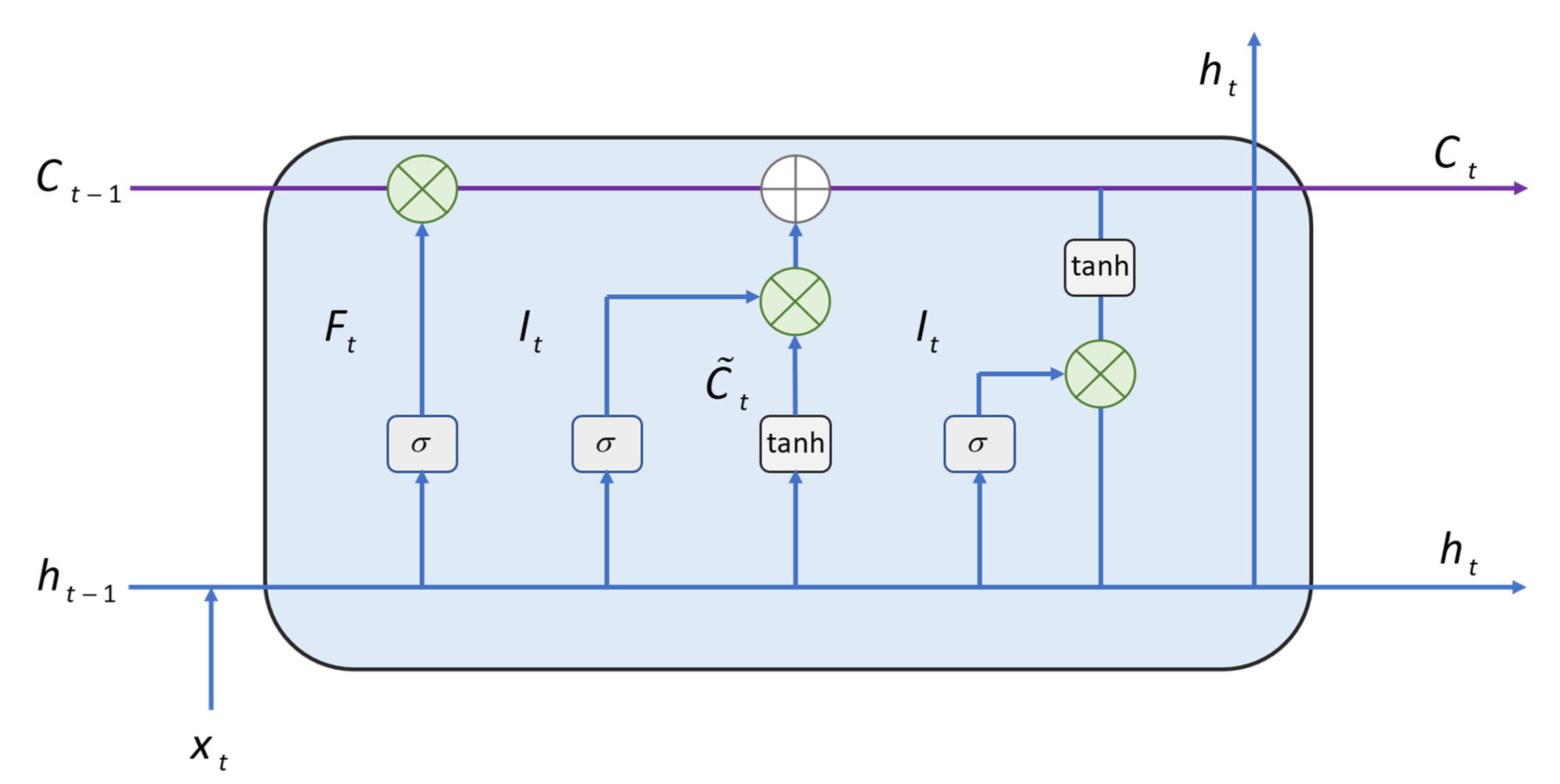
of the remote sensing image output from the encoder are fed to a decoder for decoding. The decoder can use recurrent networks (RNN), long-short term memory networks (LSTM), etc. LSTM is a special RNN, which is often chosen as the decoder of remote sensing image captioning models. As a sequential model, LSTM can learn long dependencies and overcome gradient vanishing to achieve better functionality. The information transfer in LSTM is controlled by a forget gate F t , an input gate I t and an output gate O t . The forget gate F t controls whether to clear the current value, the input gate I t determines whether to obtain new input information, and the output gate O t determines whether to output a new value. The structure of the LSTM at time t and the parameter transfer method are shown in Figure 1. At time t , the parameters in LSTM are updated as follows:
I t = σ ( W x I x t + W h I h t 1 + b I ) F t = σ ( W x F x t + W h F h t 1 + b F ) O t = σ ( W x O x t + W h O h t 1 + b O ) C ˜ t = tanh ( W x C x t + W h C h t 1 + b C ) C t = F t C t 1 + I t C ˜ t h t = O t tanh C t y t = W o u t h t
Finally, to generate word probabilities p t , we use a “softmax” layer to normalize the generated score vectors to probabilities. σ represents the nonlinear activation function sigmoid and tanh represents the hyperbolic tangent function. W x I , W h I , W x F , W h F , W x O , W h O , W x C and W h C are the trainable weight matrices in LSTM. b I , b F , b O and b C are trainable biases. W x I and W h I are the trainable weight matrices of the input gate and b I is the trainable bias of the input gate; W x F and W h F are the trainable weight matrices of the forget gate and b F is the trainable bias of the forget gate; W x O and W h O are the trainable weight matrices of the output gate and b O is the trainable bias of the output gate; W x C and W h C are the trainable weight matrices of the memory cell and b C is the trainable bias of the memory cell. The memory cell C t is used to store new state information. h t represents the hidden state of the LSTM at time t and also the output of the LSTM at time t . x t represents the input of the LSTM at time t . x t is obtained by combining h t 1 , y t 1 and the encoder-extracted feature vectors v at time t 1 in series: x t = h t 1 , y t 1 , v . h t is calculated based on h t 1 . h t 1 is calculated based on h t 2 , and so on. C t and C t 1 are also calculated in this way. When t is 0, h 0 and C 0 will be initialized to 0 before model training. h 0 , C 0 and the visual features v output from the encoder are input to LSTM for training. The word vector y t generated at time t is denoted as:
y t = W o u t h t
Word probabilities p t are normalized by softmax:
p t = S o f t m a x ( y t )
The LSTM decoder receives the features extracted from the remote sensing image by the encoder and generates the first word. The word embedding vector of the first word is passed to the LSTM as the new input for generating the second word. The decoder generates one word at each step, resulting in a textual description of the remote sensing image.
In the above encoder-decoder framework, the choice of encoder and decoder structures is not limited to the combination of CNN (ResNet) and LSTM, as described above. Various attention mechanisms are added to the LSTM to constitute new decoders. Transformers [58] and models built based on a transformer (such as bert) have achieved great results in the field of natural language processing in recent years, and the decoder can also choose a transformer instead of LSTM. The encoder can also choose from different feature extraction networks, including CNNs with various attention models attached or even a transformer-based design, vision transformer. Using these powerful new designs to construct the baseline for image captioning has great potential to achieve strong performance. However, discussing the construction of encoders and decoders is not the focus of this study. Here we choose ResNet as the encoder and LSTM as the decoder for the baseline model of the few-shot remote sensing image captioning model. After setting the overall framework of few-shot remote sensing image captioning, we improve the performance of the few-shot remote sensing image captioning model from four perspectives: feature, temporal, manner, and optimization according to the characteristics of few-shot remote sensing image scenarios.

3.1. Feature: Self-Supervised Learning

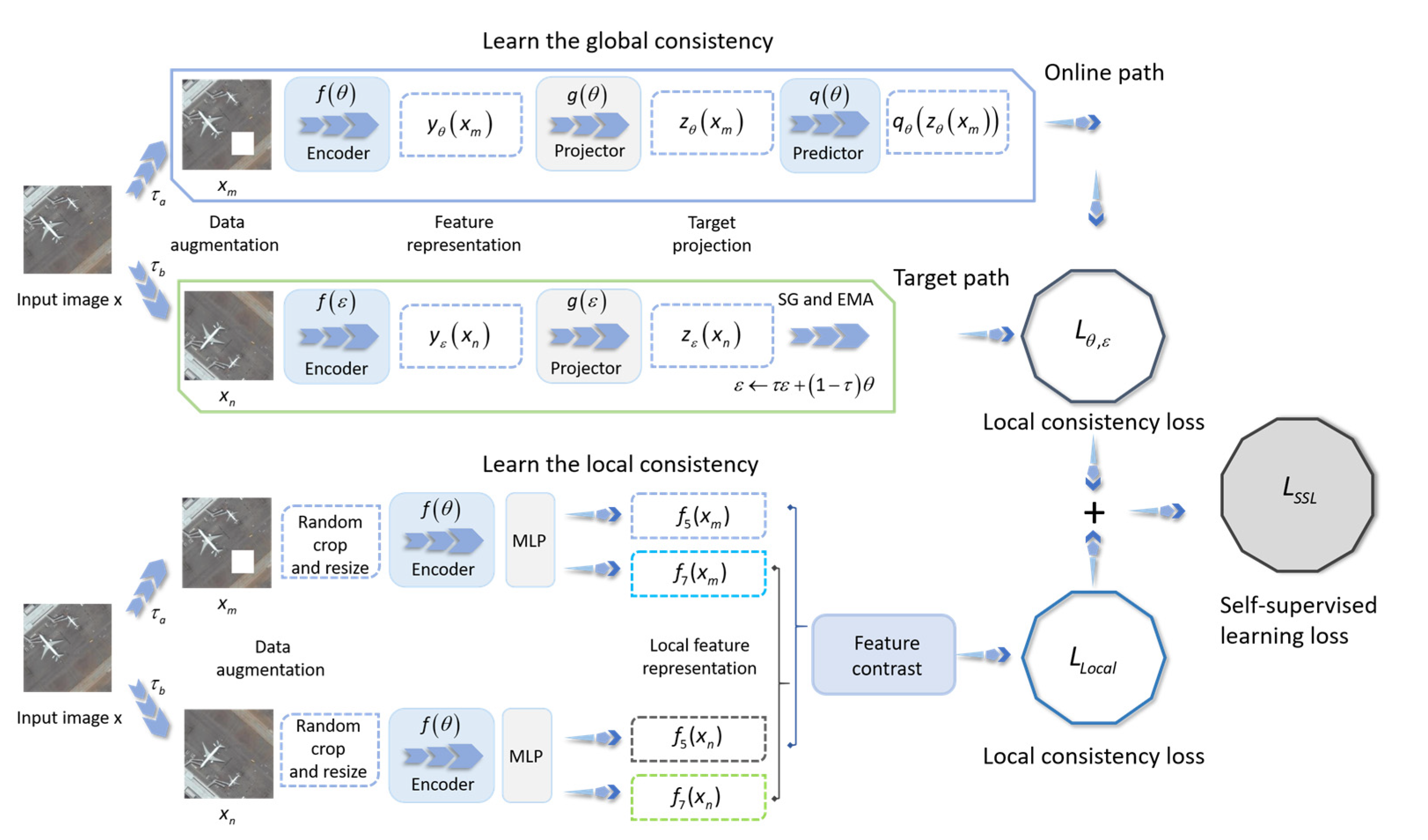
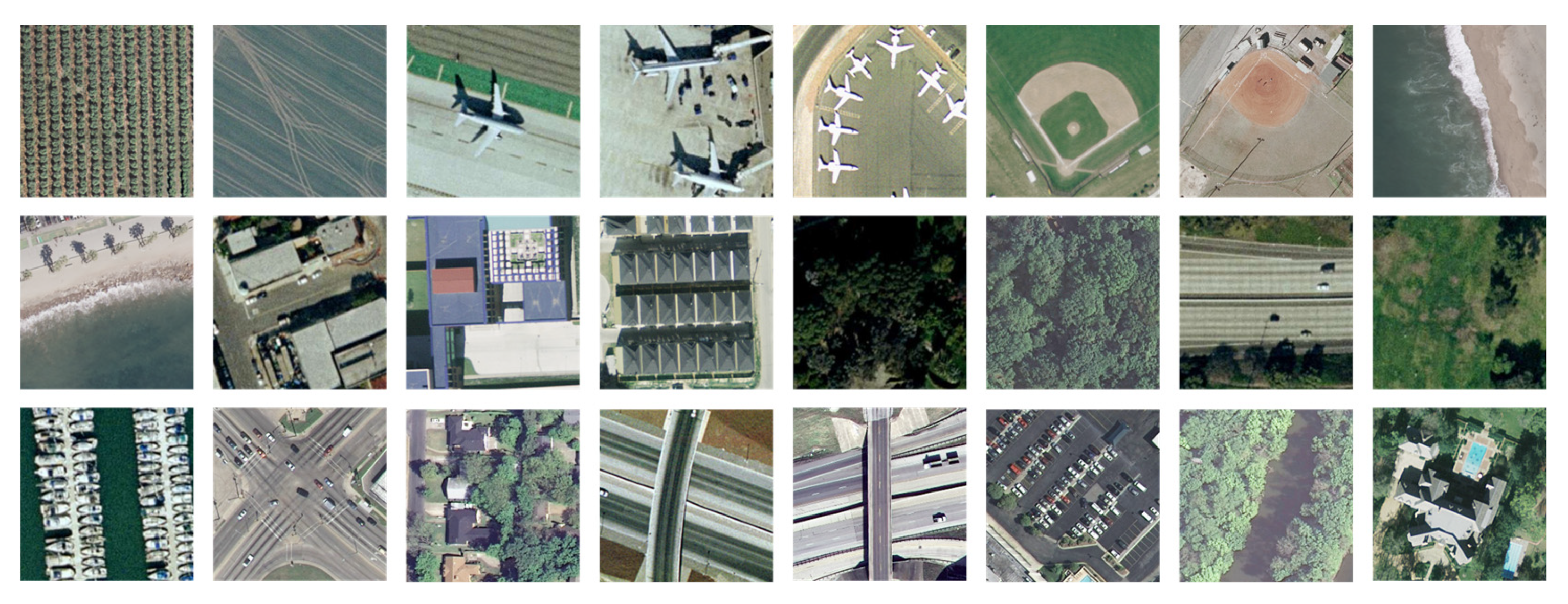
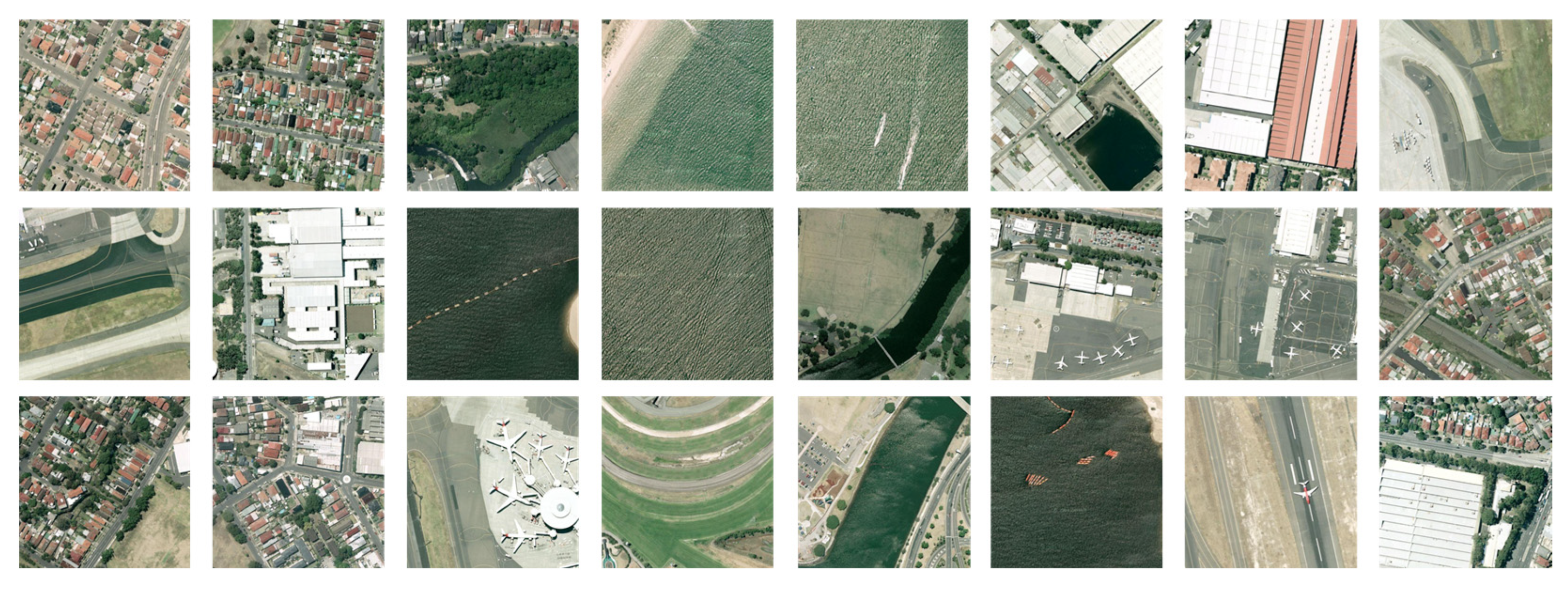
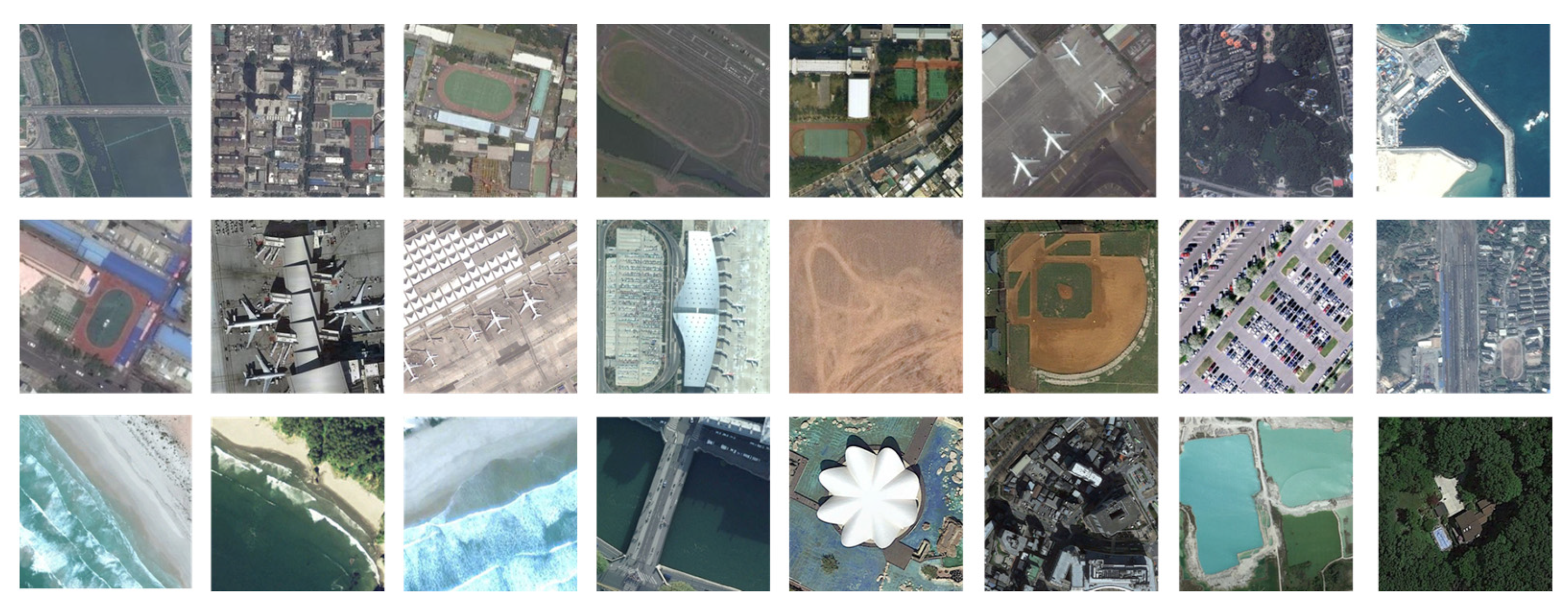
We first improve the performance of the image captioning encoder in few-shot remote sensing image scenarios from the perspective of feature extraction. The remote sensing image captioning model based on the encoder-decoder structure needs the visual features of remote sensing images for text generation. This visual feature is the same as the visual feature used in the process of the remote sensing image scene classification process. Therefore, the remote sensing image feature extraction problem in few-shot scenarios can be transformed into a few-shot remote sensing image scene classification problem to be solved. In the few-shot scenario we set, only a small number of unlabeled remote sensing images can be used to train the remote sensing image scene classification model. We note that self-supervised learning can learn generic feature information contained within the data without using label information, providing a stable and generalizable feature representation for downstream tasks. As can be seen, the goal of both self-supervised learning and few-shot learning is to reduce the reliance of model training on labeled data. Therefore, our strategy is to use self-supervised learning to train a scene classification model as an encoder in a small amount of unlabeled remote sensing image samples. We choose the classical ResNet-101 as the structure of the encoder. ResNet-101 still performs brightly in real scenarios, combining accuracy and simplicity. After determining the structure of the encoder, we need to consider how to train the encoder using unlabeled remote sensing images. Here we use self-supervised learning to further improve the encoder’s generalization ability. Self-supervised learning performs consistency regularization on the encoder, focusing on the output of the encoder rather than the specific data labels for training. Here we borrow the self-supervised training paradigm from BYOL. Without changing the original model structure, the performance of the model is improved from the data without class labels.
Given an input remote sensing image, here denoted as x , we randomly adopt two different strategies τ a and τ b for data augmentation to obtain x m and x n . The two different data augmentation strategies adopted are derived from the strategies expounded in Section 4.3. Regarding implementation details, the self-supervised learning model contains two-path modules: an online model and a target model. First of all, they both have encoders with the structure of ResNet-101, but the difference is the parameters of the encoders. Here, the encoder in the online model is denoted as f θ , and θ is the parameter of the online model. The encoder in the target model is denoted as f ε , and ε is the parameter of the target model. We input x m and x n to f θ in the online model and f ε in the target model, respectively. The role of f θ in the online model is to extract the remote sensing image y θ x m from x m . Then, we input y θ x m into the projection layer g θ to project into a higher dimensional space to obtain the vector z θ x m . In the target model, a vector z ε x n is obtained by replacing θ with ε with the same structure. The structure of the projection layer g θ and g ε is a multilayer perceptron (MLP). The divergence between the online model and the target model occurs in the next step: the online model uses z θ x m to predict z ε x n output from the target model through an additional prediction layer q θ . The prediction layer q θ is structured as a multilayer perceptron like the projection layer g θ . z ε x n stops the gradient descent and updates the parameters with momentum through ε :
ε τ ε + 1 τ θ
where τ is the decay rate, and the value is taken in [0,1]. This exponential moving average update strategy takes the target model as a mean teacher. The mean teacher constantly generates pseudo labels to serve as learning guidance and prediction objectives for the online model. The error L θ , ε generated by the prediction is calculated as:
L θ , ε 2 2 q θ z θ x m , z ε x n q θ z θ x m 2 z ε x n 2
The difference between the predicted value and the target value is continuously reduced by continuously reducing L θ , ε to a minimum value. Stop gradient means that we do not allow the generated gradients to be back-propagated at each stochastic optimization step. We minimize L θ , ε with respect to θ only, but not τ . The gradient generated by the target path will not be passed to, that is, stop the gradient descent of this path. Only the gradients passed backwards by the online path are updated. The stop-gradient design prevents the output of the target path and the online path from collapsing to the same, ensuring that self-supervised learning proceeds smoothly. At the end of the training, only the encoder f θ in the online model is saved.
Although BYOL can excellently improve the performance of the model in unlabeled data scenarios, BYOL does not take into account the local features in remote sensing images. L θ , ε can be regarded as a global consistency loss. Local features are very important for the interpretation and application of remote sensing images, which are related to the capture and extraction of key targets. Therefore, we add additional learning of the local consistency of remote sensing images to BYOL to complement the model’s ability to extract local features of remote sensing images. Figure 2 shows the schematic diagram of our self-supervised learning process.
In the process of the additional self-supervised learning, we directly select the local features extracted from remote sensing images for contrast learning. We also enhanced the input remote sensing images to get a large number of positive and negative pairs and input them into the classification model. The positive samples come from different data augmentation results of the same remote sensing image, and the negative samples are data augmentation results of different remote sensing images. A remote sensing image x is enhanced with different strategies to obtain x m and x n . We randomly crop x m to obtain a 5 × 5 slice and adjust back to the original size of x m to obtain x m 5 . We randomly crop x n to obtain a 7 × 7 slice and adjust it back to the original size of x n to obtain x n 7 . Subsequently, x m 5 and x n 7 are fed into the scene classification model (encoder) f θ for self-supervised learning based on feature comparison. Note that the encoder structure is the same for both x m 5 and x n 7 , and the parameters of the encoder are both θ . The encoder f θ is followed by an MLP for feature projection. Symmetrically, randomly crop x m to obtain a 7 × 7 slice and adjust back to the original size of x m to obtain x m 7 . Randomly crop x n to get a 5 × 5 slice and adjust back to the original size of x n to obtain x n 5 . We adopt the same treatment as above for x m 7 and x n 5 .The loss function L L o c a l generated in this process is calculated as follows:
L ( f 5 ( x m ) , f 7 x n ) = l o g exp d f 5 x m , f 7 x n x N x x n + exp d f 5 x m , f 7 x L ( f 7 ( x m ) , f 5 x n ) = l o g exp d f 7 x m , f 5 x n x N x x n + exp d f 7 x m , f 5 x L L o c a l = L ( f 7 ( x m ) , f 5 x n ) + L ( f 5 ( x m ) , f 7 x n )
where N x represents the negative samples of remote sensing image x , and d is the square of Euclidean distance. f 5 represents the feature extracted by inputting x m 5 or x n 5 into the encoder f θ and the MLP, and f 7 represents the feature extracted by inputting x m 7 or x n 7 into the encoder f θ and the MLP. f 7 ( x m ) , f 5 x n and f 5 x m , f 7 x n represent positive pairs. f 5 x m , f 7 x includes positive pairs and all negative pairs, and L is the InfoNCE loss. By continuously reducing L L o c a l to promote the realization of local consistency, only the decoder f θ is saved after training. It is important to note that there is more than just the choice of f 5 or f 7 for contrast learning. Different choices for the size of cutting and the combination of contrast can constitute different contrast learning strategies. The reason we choose them here is that using f 5 and f 7 with smaller sizes for contrast learning can reduce the occupation of computing resources. Using f 5 and f 7 with small sizes is beneficial to learn the local consistency of remote sensing images. At the same time, the difference between f 5 and f 7 , which are close in size, will not be so large that it is too difficult for the encoder to learn. Finally, more f 5 and f 7 with smaller sizes can be generated from one image, which is conducive to alleviating the few-shot problem.
Therefore, considering the global consistency of the model to the images and the local consistency of the features, we implement self-supervised learning with decreasing L θ , ε and L L o c a l by gradient descent until a minimum value is reached. At the end of the training, only the encoder f θ is retained. Self-supervised learning helps the encoder learn a general feature expression from a small number of unlabeled remote sensing images for remote sensing image scene classification. The semantic features are extracted from a limited number of remote sensing images using the encoder with caption labels but without class labels. Then the extracted semantic features are input into the decoder to generate captions. The decoder only needs to focus on generating captions for limited caption-labeled samples.

3.2. Temporal: Self-Ensemble

After optimizing the feature extraction process of the encoder, we improve the performance of the decoder in the image captioning method in few-shot scenarios from a temporal perspective. Better performance is often achieved by ensemble training models. However, the usual ensemble training needs to integrate the outputs of multiple pre-trained models, which leads to a high cost of training and is not suitable for the few-shot scenarios. Therefore, we adopt self-ensemble training, which is more suitable for the set few-shot scenarios. Considering that the text generation model is sequential, we regard the different forms of image captioning models in different training stages as different models and then ensemble these models. In order to reduce the complexity of the model and improve the accuracy of the model [59], we use parameter averaging instead of directly averaging the output of the model to achieve a self-ensemble of the model. We use the model in the training process to generate a series of pseudo labels and construct a mean teacher with exponential moving average (EMA) through the consistent regularization of the model itself in the training process as a self-ensemble model to guide the model for more in-depth training. The self-ensemble image captioning model F S E is defined as:
F S E x | θ k ¯ = F S E x | 1 t t = 1 t θ k t θ k ¯ = 1 t t = 1 t θ k t
where x is the input image, t is the time step of training, θ k is the parameter of the model at the k-th time step, and θ k ¯ is the average parameter of the model within t recent time steps. The expression for θ k ¯ can be expressed by a constant transformation as:
θ k ¯ = α θ k 1 ¯ + ( 1 α ) θ k
It can be found that the updating process of θ k ¯ can be seen as using EMA to train a mean teacher with a smoothing coefficient of α as a self-ensemble model. The introduction of the parameter moving average self-ensemble can improve the accuracy of captions generated by the model and further reduce the dependence of the model on labeled samples.

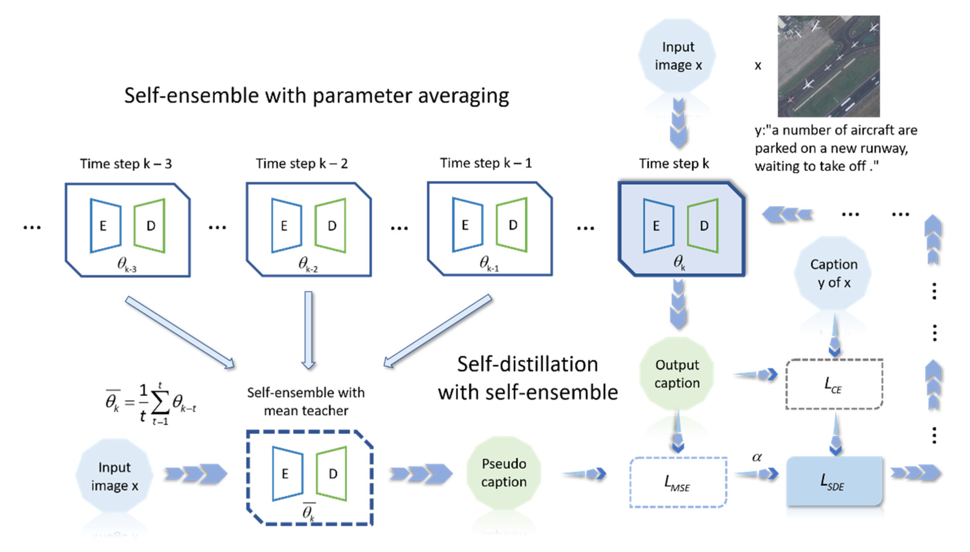
3.3. Manner: Self-Distillation

After using self-ensemble to improve the performance of the model from a temporal perspective, we further optimize the training manner of the model. Knowledge distillation can transfer knowledge from the teacher model to the student model. When the teacher model and the learning model have the same structure, knowledge distillation becomes self-distillation. Self-distillation eliminates the need to train additional models, additional prior knowledge and additional training data. Knowledge is transferred from the previous generation model to the next generation model in the form of pseudo labels. Model performance can be improved through multiple iterations. These characteristics of self-distillation can well alleviate the pain points of few-shot scenarios. We combine self-distillation with the above self-ensemble: unlike the common self-distillation in which the teacher model and the student model directly adopt the same structure, we use the model obtained from the self-ensemble as the teacher model to train the next generation of student models. A series of pseudo semantic annotation labels generated by the self-ensemble model is fed to the self-distillation model for training, and the self-distillation will continue to generate new pseudo semantic caption labels to store in the performance boost of the next-generation model. The loss function L S D E of self-distillation combined with self-ensemble in the process of training the model F S D E x is:
L S D E = L C E y , F S D E x | θ k + β L M S E F S D E x | θ k , F S E x | θ k ¯ θ k ¯ = 1 t t = 1 t θ k t
where x represents the input image, y represents the semantic annotation label of x , L C E represents the cross-entropy loss, L M S E represents the mean square error, θ t represents the parameters of the t generation model, and β is used to adjust the proportion of cross-entropy loss and mean square error. θ t ¯ represents the averaged parameters in the first t time steps, including the k-generation model. The hyperparameter t determines the scale of self-ensemble with parameter averaging.
The schematic diagram of the self-distillation training strategy with self-ensemble is shown in Figure 3. In the training process, θ t ¯ will change with the advance of the training step, which can prevent the model from overfitting. The performance obtained from self-distillation training will also be self-ensembled into the training of the next-generation model. Self-ensemble and self-distillation can promote each other in this process so that the training of the model tends to be stable, and finally, we obtain a model with the best performance in the training process.

3.4. Optimization: Self-Critical

In this section, the performance of the image captioning model is improved through parameter optimization of the image captioning model. There are several problems in the training and testing process of image captioning from few-shot remote sensing images. First, in the few-shot scenarios, the data distribution of the model does not match the process of training and testing. Because the total number of remote sensing image samples with caption labels is small, the number of samples with caption labels that can be obtained in the training stage is correspondingly small. The train set is expanded in various ways, but the train set will not be changed. The data distribution of the train set and the test set is different. In the process of training the image captioning model, the model will predict the next word based on the generated words and use gradient descent to continuously optimize the model. In this process, the difference in data distribution between the train set and the test set will be further accumulated. During the training process, the input of the model is all from the real dataset, and the labels of the samples are ground truth. However, the input of the model in the test process comes from the output of the previous time. The errors generated in the test process will continue to accumulate. This phenomenon is called exposure bias [54]. Second, the image captioning model uses a loss function to tune the model parameter θ during the training process but uses evaluation metrics such as BLEU, CIDEr, ROUGE, and SPICE to evaluate the performance during the testing process. These metrics are non-differentiable with respect to the parameter θ , so it is not possible to use gradient descent to feed the test results directly to the model for optimization.
Several studies have shown that the policy-gradient method in reinforcement learning can be used to solve the problems of exposure bias and the non-differentiability of training metrics. Reinforcement learning defines a text generation model as an agent that interacts with the “environment”, defines descriptive captions and remote sensing image features as the “environment”, and considers the evaluation metric CIDEr score of descriptive captions as the reward R w . The policy gradient method expresses the learning policy as F θ using the parameter θ . The training expectation function is:
L θ = E F θ R w s
where w s = W 1 s , W 2 s , , W T s . w s represents sequentially generated word sequences (sentences), W t s denotes the generated words sampled from the model using strategy F θ at time t, and E F θ denotes negative expectation. The reward is adjusted by introducing a baseline b of the greedy decoding output to calculate the reward gradient estimation with feedback from the strategy parameters and the environment to achieve an optimal update of the parameter θ and finally obtain the maximum cumulative reward. The gradient estimate on θ is:
θ L θ R w s b θ log F θ w s
The baseline b can be any function independent of w s . The introduction of b can reduce the variance of the gradient estimate. This is an end-to-end method to search for the optimal solution in the policy space, which has a wide range of applications. This method also has obvious shortcomings: the gradient variance calculated under the reinforcement learning framework is very large. The training is very volatile, and the model is easy to converge to a local minimum, which is similar to the phenomenon of overfitting, resulting in poor quality of the generated captions. These disadvantages can be magnified in few-shot scenarios.
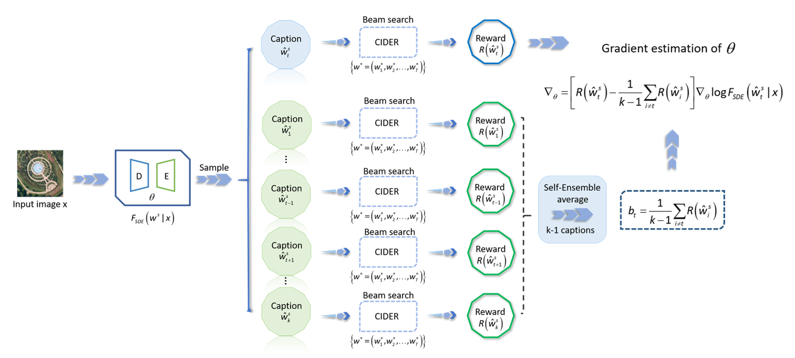
To solve the above problems, we adopt the self-critical paradigm [57] proposed in the self-critical sequence training for image captioning (SCST) to optimize the process of using reinforcement learning to train the image captioning model. The self-critical technique in SCST introduces a baseline calculated by greedy search, which can reduce the gradient variance. The self-critical technique adjusts the baseline according to the greedy decoding output of the image captioning model in the test reasoning process and finally optimizes the image captioning model, achieving superior performance to the vanilla reinforcement learning. Ref. [57] shows that the variance of the self-critical model is very small, and good results can be achieved in few-sot samples with the use of SGD. At the same time, the self-critical technique realizes the direct measurement of sequence variables by adjusting the baseline and promotes consistency in the process of training and testing. The optimization goal in self-critical training is to maximize the CIDEr scores of the generated captions. We follow this design, but different from the greedy search used in SCST to calculate the baseline, we simultaneously sample multiple captions of the same remote sensing image by the model and calculate a baseline with self-ensemble according to the beam search [60]. The schematic diagram of using self-critical to optimize model parameters is shown in Figure 4.
For few-shot remote sensing scenarios, we collect K captions of the input remote sensing image x generated by the model F S D E ( x ) after self-ensemble and self-distillation training: w ^ 1 s , w ^ 2 s , , w ^ k s , w ^ t s F S D E w s | x . The caption label corresponding to the input remote sensing image x is w = w 1 , w 2 , , w T . When calculating the CIDEr scores of these K captions, we use beam search instead of greedy search. Beam search has a larger search space than greedy search. It does not pursue local optimization but global optimization. The speed and accuracy of training are better than greedy search. Beam search is very useful in scenarios where there are obvious differences in the data distribution between training samples and test samples [3], and the few-shot scenario is one of them. Compared with greedy search, the calculation method of beam search can avoid the continuous accumulation of errors to a certain extent and reduce the adverse effects of exposure bias. We integrate the self-ensemble calculation method into the baseline calculation process as follows: we randomly select a caption w ^ t s , and the baseline b t of caption w ^ t s is obtained by the average integration of the reward CIDEr scores of other K-1 captions:
b t = 1 k 1 i t R w ^ i s
where R w ^ i s is the CIDEr score of w ^ i s . Because the K captions and the corresponding CIDEr scores are generated by the same model based on a remote sensing image, they are independent of each other. Therefore, the calculation of b t does not depend on w ^ i s , and b t is a valid baseline. The self-ensemble here averages the scores of multiple captions generated by the model for the same input image. The gradient estimation of the parameter θ of model F S D E ( x ) is calculated as:
θ R w ^ t s b t θ log F S D E w ^ t s | x = R w ^ t s 1 k 1 i t R w ^ i s θ log F S D E w ^ t s | x
Self-critical techniques using the baseline obtained from the self-ensemble model can improve the utilization of limited samples and effectively avoid the possible overfitting caused by few-shot problems. At the same time, it can further reduce the gradient variance in the reinforcement learning process and better optimize the few-shot remote sensing image captioning model.

4. Experiments

In this section, we present a series of experiments we have implemented and the experimental results. The experimental results prove the effectiveness of our SFRC method in few-shot remote sensing scenarios. First, we clarify the selection of datasets in the experiments and the evaluation metrics used in the experiments to evaluate the generated remote sensing image captions. Then, we introduce the details of the implementation of the experiment, including the software and hardware parameters of the experimental equipment, the preprocessing of data, the structural parameters of the model, the setting of super parameters, and so on. Next, we conduct a series of quantitative experiments to compare the SFRC method with classical and recent methods. We also perform percentage sampling experiments to observe the performance of the SFRC method when the available data are further reduced. Finally, we conduct a series of ablation experiments to analyze the effectiveness and necessity of various components in the SFRC method.

4.1. Dataset

We selected the RSICD dataset, UCM-Captions dataset, and Sydney-Captions dataset as the datasets for training, validating and testing the few-shot remote sensing image captioning tasks. Their samples are all RGB images containing manually annotated captions.

4.1.1. UCM-Captions Dataset

The UCM-Captions dataset was constructed based on the UCM-Merced University Land-Use dataset [61]. The images are from the national map urban area of the United States Geological Survey. The UCM captions data set contains 21 categories, including aircraft, beaches, overpasses and stadiums, with a total of 2100 remote sensing images. Some samples in the UCM captions dataset are shown in Figure 5. Each remote sensing image has a resolution of 256 × 256 pixels and is equipped with 5 different caption labels. The entire dataset uses 368 different words to generate 10,500 caption labels in describing the images.

4.1.2. Sydney-Captions Dataset

The Sydney-Captions dataset was collected and produced in Google Earth’s Sydney dataset [62]. Each remote sensing image was cropped from the 18,000 × 14,000 pixel remote sensing image of Sydney, Australia, with a resolution of 500 × 500 pixels. Some samples of the Sydney-Captions dataset are shown in Figure 6. The Sydney-Captions dataset contains a total of 613 remote sensing images, which are divided into 7 categories, such as airports, oceans, and factories. This dataset uses 237 different words to generate five different caption labels for each remote sensing sample. This dataset has more detailed description statements, but there is a problem in that the number of remote sensing samples is small.

4.1.3. RSICD Dataset

The RSICD dataset [18] is composed of remote sensing images collected from Google Earth, Baidu Maps, MapABC, and Sky Map (Tianditu) in 2017 and divided into 30 scene categories. Each remote sensing image is 224 × 224 pixels. Some samples of the RSICD dataset are shown in Figure 7. The RSICD dataset is the largest dataset for remote sensing image captioning tasks at present. The linguistic descriptions of remote sensing images in this dataset are more relevant because these descriptions do not contain pre-defined observation directions and vague adjectives, using a total of 3325 different words. Some of the samples in the dataset correspond to five different caption labels. Samples with less than five semantic captions were complemented to five annotations by copying existing captions. Finally, the whole dataset contains 10,921 images and 54,605 corresponding remote sensing annotation statements.
The captions sampling in the three datasets are shown in Figure 8 and Figure 9. Combining the number of samples in each dataset, we find that each remote sensing sample in the UCM-Captions dataset and Sydney-Captions dataset is configured with sufficient captions, but the number of remote sensing samples in these two datasets is too small. The RSICD dataset contains a not very small number of remote sensing image samples, but some of the samples are not equipped with a sufficient number of captions. From the perspective of providing effective supervision information for model training, these three datasets are still small compared with the natural image captioning datasets. The methods are prone to overfitting problems in these datasets due to the sparse samples. Therefore, it is reasonable and feasible for us to use these datasets to train, validate and test the few-shot remote sensing image captioning methods. Here we will pay special attention to the results of the methods in the Sydney-Captions dataset containing definitely sparse samples.

4.2. Evaluation Metrics

When evaluating the quality of remote sensing image captions, we select BLEU, ROUGE, CIDEr, SPICE, and METEOR as evaluation metrics.
BLEU (Bilingual Evaluation Understudy): BLEU is an evaluation metric for machine translation proposed by IBM in 2002 [63]. It can evaluate co-occurrences between generated captions and ground truth captions. According to the n-gram matching rules, BLEU-1, BLEU-2, BLEU-3 and BLEU-4 are calculated to measure the accuracy of word translation and the fluency of generating description sentences. BLEU’s rating range is 0–1.
ROUGE (Recall-Oriented Understudy for Gisting Evaluation): ROUGE is a similarity measurement method based on recall rate [64], which is used to evaluate the accuracy of the generated description statements. There are four main types of ROUGE: ROUGE_N, ROUGE_L, ROUGE_ W, and ROUGE_S. In this paper, ROUGE_L was chosen as the evaluation metric, which calculates an F-measure with recall bias for the longest common subsequence (LCS) between the generated captions and the ground truth captions. ROUGE_L is scored in the range of 0–1.
CIDEr (Consensus-based Image Description Evaluation): CIDEr is a metric designed specifically for evaluating image captioning tasks [65]. It evaluates the consistency of description through term frequency-inverse document frequency (TF-IDF) calculation. CIDEr gives less weight to frequently occurring specific n-grams that do not contain useful visual information, mainly to judge whether the captions contain key information. CIDEr is popular among researchers because of its ability to evaluate whether the generated captions conform to human preferences. In order to prevent the occurrence of the “gaming” problem [65], the researchers optimized the CIDEr by introducing the Gaussian penalty for the length difference between the generated captions and the ground truth captions. The optimized CIDEr is more popular, and its score range is 0–10.
SPICE (Semantic Propositional Image Caption Evaluation): SPICE is also specifically designed to evaluate image captioning tasks [66]. SPICE maps both ground truth captions and generated captions into a scene graph to evaluate the correlation between them. As a graph-based semantic representation, the scene graph can encode targets, attributes, and relationships in the generated captions. The score range of SPICE is 0–1.
METEOR (Metric for Evaluation of Translation with Explicit Ordering): METEOR calculates the accuracy and recall rate of the unigram alignment between the generated captions and the ground truth captions based on the whole corpus and generates a harmonic mean [67]. Unlike BLEU, meteor calculates the word-to-word match relationship between generated captions and ground truth captions. METEOR is widely used in image captioning and can be considered a modified version of BLEU. METEOR has a rating range of 0–1.
The higher scores of the above evaluation metrics, BLEU, ROUGE, CIDEr, SPICE, and METEOR, indicate that the more accurately the generated caption describes the images (remote sensing images), the closer the description method is to human description habits.

4.3. Implementation Details

The experimental device we used was equipped with an Intel Core i9-10900K @ 3.70 GHz as the CPU. The GPU model was an NVIDIA GeForce RTX3090, which was released by NVIDIA in 2020, with 24 GB GDDR6X video memory and 384-bit memory width. The computer memory was 16 GB DDR4 3200 MHz × 4, 64 GB in total. The total capacity of the hard drive was 2 TB. We deployed the Ubuntu 20.04 LTS operating system in the above experimental equipment, and the deep learning framework adopted was Pytorch 1.8.
When using self-supervised learning to train the scene classification model, the unlabeled remote sensing samples we used came from the above remote sensing image captioning datasets. We did not use the captions in the datasets; we only used the remote sensing samples in the datasets. From our analysis of three remote sensing image captioning datasets, we can see that although these samples are not labeled with class labels for classification, they are actually sampled from different remote sensing scenes. For example, the remote sensing samples in the RSICD dataset can be divided into 30 different scenes. This allows us to use these unlabeled data to train the self-supervised learning scene classification model. We divided these samples into two sets: the train set, composed of 70% samples, and the test set, composed of 30% samples.
We adopted various data augmentation strategies in the process of self-supervised learning. Our data augmentation strategies for the input remote sensing images included Cutout [68], randomly cropping and resizing the remote sensing images, converting the remote sensing images to grayscale with 50% probability, randomly flipping the remote sensing images with 50% probability, adjusting the brightness, contrast, saturation, and hue of the remote sensing images using the ColorJitter tool, adding Gaussian blur with 20% probability and so on. Random augmentation, probabilistic augmentation and different combinations can produce many different strategies. We used these data augmentation strategies in our experiments. Of course, this order can be changed.
We loaded ResNet-101 from the torchvision module in Pytorch as the initial structure of the encoder f θ for self-supervised learning. In the training process of BYOL, both the prediction layer q θ and the projection layer g θ use MLP architecture. We set the structural parameters of the MLP that constitutes the prediction layer and the projection layer to be the same: the projection size was set to 256, and the projection hidden size was set to 4096. The decay rate of the mean teacher τ was initially set to 0.996 and gradually increased to 1.000 during the training process. In the local feature extraction capability enhancement part of the self-supervised learning, the structure and parameters of the encoder were the same as those of the encoder f θ in the BYOL part. The MLP behind the encoder had the same structure and parameters as the projection layer g θ in the BYOL part. The Adam optimizer was chosen for the whole training process, and the learning rate was set to 3 × 10⁻⁴. The training batch size was 32, and a total of 200 epochs were trained.
When the training model generated captions for few-shot remote sensing samples, we divided the three remote sensing caption datasets into a train set, validation set and test set. Among them, the samples used for training account for 80%, the data used for validation account for 10%, and the data used for testing account for 10%.
The hidden state dimension, image feature dimension and word embedding dimension in the LSTM model we used as the decoder were all fixed to 512. The sliding momentum coefficient α in the self-ensemble process was taken as 0.99, and the hyperparameter β in the self-distillation process was taken as 1. Just like the self-critical design idea we designed in Section 3.4, the evaluation metric used to guide the optimization of the model parameters in the model training process was CIDEr. We trained the model to obtain a maximum CIDEr score and then used CIDEr together with other metrics to evaluate the quality of the generated remote sensing captions. When calculating the CIDEr score baseline in the self-critical technique, we sampled 5 captions for each remote sensing image. The beam size of the beam search was taken as 5. The optimizer we used was Adam with weight decay, and the initial learning rate was 2.5 × 10⁻⁴. The weight decay was set as 5 × 10⁻⁴. A total of 100 epochs were trained. During this period, the learning rate was annealed by a factor of 0.8 every 3 epochs. The batch size during training was set to 30.

4.4. Quantitative Results

We conduct quantitative comparison experiments between our proposed SFRC method and some classical remote captioning methods as well as recently proposed methods in each of the three datasets. These methods include soft attention [18], hard attention [18], RNNLM [69], AoANet [70], SAT [71], FC-Att + LSTM [72], SM-Att + LSTM [72], sound-a-a [73], RTRMN [74], M-M-GRU [75], SAT(LAM) [76], and multi-level ATT [77].
Ref. [18] mentioned two remote sensing caption generation algorithms, soft attention and hard attention. Both methods use the encoder-decoder architecture: the encoder adopts VGG-16, and the decoder adopts LSTM. The difference between them lies in the attention mechanism used. Soft attention determines a certain area of remote sensing image through a certain weight. Hard attention uses a sampling strategy to focus on remote sensing images and uses reinforcement learning to train the model. Soft attention and hard attention are two classical and widely used remote sensing image captioning methods.
The RNNLM method proposed by [69] first uses the convolutional neural network CaffeNet to obtain labels containing the main targets in the remote sensing images and then uses the RNN to generate descriptive sentences about the important targets.
Ref. [70] proposed an AoA attention module. This module uses a self-attention mechanism to measure the correlation between image features. The AOA module is applied to the encoder and decoder in the caption generation model at the same time. At this time, the network is named AoANet.
In [71], a classical attention-based image captioning model, Show-Attend-and-Tell (SAT), is proposed. SAT extracts features from the middle layer of the convolutional neural network to feed into the LSTM containing an attention mechanism for image captioning.
FC-Att + LSTM and SM-Att + LSTM were proposed by [72]. They all use an attribute attention mechanism to process the high-level semantic features in remote sensing images and use the extracted high-level attributes to generate description statements. The difference between FC-Att + LSTM and SM-Att + LSTM is the output source of their high-level attributes. The mid-level and high-level attributes of FC-Att + LSTM come from the last full connection layer of the CNN. The mid-level and high-level attributes of SM-Att + LSTM come from the softmax layer of the CNN.
The sound-a-a method, proposed by [73], is an active attention mechanism constructed from sound. The sound information processed by the attention module can guide the model to generate descriptive sentences of interest to the observer. Both the sound module and the attention module in sound-a-a contain gated recurrent units (GRU).
The RTRMN method in [74] is designed to overcome the problem of long-range information dilution in RNNs. The RTRMN uses a topic word strategy to extract topic information from the captions corresponding to the input remote sensing images and then feeds this topic information into the RNN to generate captions to the remote sensing images.
M-M-GRU was proposed by [75], which has a convolutional neural network as the encoder and gated recurrent units (GRU) as the decoder. This method uses the image features extracted by the convolutional neural network to generate descriptive sentences that can vary in length.
Unlike the conventional attention caption generation model, SAT (LAM) [40,76] uses the LAM method additionally. The LAM method does not use high-level remote sensing image features to guide the attention calculation process. LAM implicitly introduces additional label information into the model, which can help the attention mechanism better focus on important areas and key categories and provide more useful semantic information for the model to generate description statements.
Ref. [77] proposed a multi-level ATT mechanism imitating human beings to generate remote sensing image captions. This attention mechanism includes attention to remote sensing image areas, words and semantic information. The encoder is ResNet, and the decoder is LSTM.
In Table 1, Table 2 and Table 3, the highest scores under each evaluation metric are marked in bold. For these methods used for quantitative comparison with SFRC, their evaluation metric scores are derived from their paper experimental results. Of these, soft attention [18] and hard attention [18] do not provide SPICE scores in the original paper, and these scores are replaced with “-” in Table 1, Table 2 and Table 3. As can be seen from Table 1, Table 2 and Table 3, our proposed SFRC received the highest scores in most of the metrics. Even if some index scores do not get the highest score, they are not far from the highest score and belong to the category of high scores. The high scores obtained under the BLEU-1, BLEU-2, BLEU-3 and BLEU-4 evaluation metrics of the BLEU series mean that SFRC translates words accurately and sentences smoothly. The high scores under the METEOR evaluation metric mean that the matching rate between captions generated by SFRC and ground truth captions is high, and the gap is small. The high scores under the ROUGE evaluation metric indicate that SFRC generates accurate captions. The high score for CIDEr indicates that SFRC describes key information and matches human preferences. The high score for SPICE demonstrates that SFRC accurately captures the targets, attributes and relationships in remote sensing images.
On the UCM-Captions dataset, our SFRC method achieved the highest scores for BLEU-1, BLEU-3, ROUGE, CIDEr and SPICE. This indicates that SFRC has captured key information in the remote sensing images in the UCM-Captions dataset. The multi-level ATT method achieved the highest scores for BLEU-2 and METEOR. SAT (LAM) achieved the highest score for BLEU-4. This means that there is room for improvement in the matching rate between the captions generated by the SFRC and the ground truth captions. The fluency of the generated descriptive sentences also needs to be improved.
Our SFRC method obtained the highest scores for all metrics on the Sydney-Captions dataset, which contains the fewest samples. This indicates that our series of designs for the few-shot remote sensing image captioning task is fruitful. The generated captions have high accuracies and matching rates while extracting key information and important targets from the remote sensing images.
The SFRC method obtained the highest scores for BLEU-1, BLEU-2, BLEU-3, BLEU-4, CIDEr and SPICE on the RSICD dataset. The highest scores for METEOR and ROUGE came from the multi-level ATT method. This is because the RSICD dataset contains the richest amount of words, and the attention mechanism in the multi-level ATT method facilitates the selection of appropriate words to describe the remote sensing images and generate captions that match the ground truth captions.
From the overall perspective of the three datasets, SAT (LAM) and multi-level ATT, which use a strong attention mechanism, still perform well in some metrics, especially METEOR. Our method has obtained competitive scores in most metrics, which means that the overfitting of the model in few-shot scenarios has been alleviated.
There is a widely accepted consensus that using more samples tends to mitigate overfitting to a certain extent and allows the model to perform better. However, by vertically comparing the evaluation metric scores of the same method in Table 1, Table 2 and Table 3, we find that image captioning methods usually have the highest scores on the UCM-Captions dataset, followed by the Sydney-Captions dataset, and lowest on the RSICD dataset. Although we cannot draw firm conclusions directly from the evaluation metric scores alone, these results do suggest that the RSICD dataset in all three datasets is the most difficult for the models to learn, followed by the Sydney-Captions dataset, with the UCM-Captions dataset being the easiest to learn. This is at variance with our analysis of the datasets above: using the RSICD dataset with the most remote sensing image samples and the richest descriptive sentences resulted in a model with lower evaluation metric scores. Using the UCM-Captions dataset with fewer remote sensing data samples and the simplest sentences often resulted in a model with high evaluation scores. This counter-intuitive phenomenon makes us rethink how the few-shot problems in remote sensing image captioning should be determined. It is evident from the above phenomenon that the performance of the model is also limited when the quality and quantity of remote sensing samples in the dataset equipped with ground truth captions cannot support the model for full training. This is also a few-shot problem in one sense. At the same time, excessively long descriptive sentences equipped with remote sensing images and too many total words used in the ground truth captions in the dataset will add difficulty and burden to the learning of the models, resulting in a steep increase in the quantity and quality of caption-labeled remote sensing samples required by the model. The richer the words contained in the ground truth captions, the wider the search scope in the caption generation process, and the difficulty of model learning becomes greater. This requires a larger number of training samples to support the training. The training of remote image captioning requires a balance between a sufficient number of samples and sufficient quality of ground truth captions. This can be confirmed by the metric scores of the Sydney-Captions dataset: the ground truth captions in the Sydney-Captions dataset are more detailed than those in the UCM-Captions dataset and less complex than those in the RSICD dataset. However, the Sydney-Captions dataset contains the smallest number of samples. The final metric scores in the Sydney-Captions dataset were second. Of course, the low scores of the models trained on the RSICD dataset do not mean that the qualities of the generated captions are poor. The high qualities of the ground truth captions naturally improve the criteria for evaluating the captions generated. This issue would become clearer if there were a metric for evaluating model-generated descriptive sentences that did not rely on the ground truth captions provided by the dataset.

4.5. Percentage Sampling Few-Shot Experiments

In order to further test the performance of our proposed method for image captioning in few-shot remote sensing scenarios, we conducted an in-depth exploration of the UCM-Captions dataset, Sydney-Captions dataset and RSICD dataset. We introduced percentage sampling in the model training process: the model was trained using a randomly selected percentage of samples in the dataset. This method of sampling according to a certain percentage can reduce the sampling scale and try not to change the original sample distribution of the train set. Both the UCM-Captions and Sydney-Captions datasets contain only a few hundred caption-labeled samples, which is more compatible with the definition of “few-shot” in terms of sample size. When we experiment with percentage sampling in these two datasets, the samples we can obtain will become extremely scarce. This puts forward high requirements for the ability of the method to adapt to few-shot scenarios. Therefore, we paid special attention to the results of the experiments on the UCM-Captions dataset and the Sydney-Captions dataset. We set different sampling percentages in our experiments: 60%, 80% and 100%. The percentage sampling experimental results are shown in Table 4, Table 5 and Table 6.
As seen in Table 4 and Table 5, our proposed SFRC method can still play a good role in image captioning when trained with only 80% of the caption-labeled samples in the UCM-Captions dataset and Sydney-Captions dataset. When only 60% of the caption-labeled samples are used for training, the performance of the model does not collapse. SFRC can adapt to sparse data modalities with few samples. From the overall view of Table 4, Table 5 and Table 6, SFRC does not lose too much performance in all three datasets due to the reduction of caption-labeled samples with the gradual reduction of sampling percentage. These suggest that our designs for few-shot scenarios are meaningful and effective. We also found that SFRC loses the most performance on the RSICD dataset when we reduce the sampling percentage. We think that this is consistent with our discussion in Section 4.5: the RSICD dataset with the largest sample size and the richest vocabulary is, in fact, severely insufficient in terms of model training, and the model is more prone to overfitting. Of course, these experimental results also imply that increasing the number of samples can bring some performance gains to the SFRC method. When the remote sensing samples with semantic captions are added in a certain range, self-supervised learning can better play its advantages in obtaining supervision information from the internal structure of the samples that are not class-labeled. Self-ensemble and self-distillation can produce more pseudo labels, the number of iterations of training can be increased, and the training process will become more stable. The baselines obtained by self-ensemble calculation in the self-critical technique will also become more diverse. However, this does not mean that by continuously increasing the number of remote sensing samples, the performance of the few-shot image captioning model in the test set can always be improved. When the samples become adequate, the performance of the model will be limited by the data distribution difference between the train set and the test set. If the difference between the test set and the train set is too large, increasing only the number of samples can yield a limited improvement.
In order to more clearly show the advantages of SFRC in few-shot scenarios, we also compared SFRC with the other three remote sensing image captioning methods in a series of experiments with a sample sampling percentage of 60%. The three methods used for comparison are RNNLM, AoANet and hard attention. The experimental results are shown in Table 7, Table 8 and Table 9.
It can be seen from Table 7, Table 8 and Table 9 that the SFRC method achieves its best score when only 60% of the remote sensing samples are used for training. Compared with the other three remote sensing image captioning methods, SFRC better adapts to few-shot scenarios and makes use of the limited remote sensing samples to generate nice quality description sentences. Comparing Table 7, Table 8 and Table 9 and Table 1, Table 2 and Table 3, when the sampling percentage is reduced from 100% to 60%, SFRC can still generate captions of good quality. However, the performances of other remote sensing image captioning methods are greatly reduced. The excellent performance of SFRC in percentage sampling few-shot experiments proves the effectiveness of a series of designs for few-shot scenarios.

4.6. Ablation Experiments

To explore the impact of each self-learning component of our proposed SFRC method in the remote sensing image captioning tasks with sparse samples, we also designed a series of ablation experiments in the three datasets. We set up four methods for ablation comparison. They were the complete SFRC method we propose, the SFRC method with the self-supervised learning part removed and the rest unchanged (No SSL), the SFRC method with the self-ensemble and self-distillation parts removed and the rest unchanged (No SE and SD), and the SFRC method with the self-critical part removed and the rest unchanged (No SC). Self-ensemble and self-distillation are combined here because they are mutually coupled and contribute to each other during the operation of the SFRC method. Self-ensemble itself is also a part of the self-distillation design. Therefore, in the ablation of the components here, we process the self-ensemble and self-distillation simultaneously rather than separately. A comparison of the evaluation metric scores of the captions generated by each method on the three datasets in the ablation experiments is shown in Table 10, Table 11 and Table 12.
We select the experimental ablation results (Table 11) of the model in the Sydney-Captions dataset with the least number of samples as the example for quantitative analysis. Self-supervised learning changed the CIDEr score of the algorithm on the Sydney-Captions dataset from 2.5936 to 2.6388, an improvement of 1.7%. SPICE score changed from 0.4359 to 0.4445, an increase of 1.9%. This demonstrates the effectiveness of using a small number of unlabeled samples for a self-supervised learning training encoder. However, the effect is not very prominent. This is the result of not using a large amount of additional remote sensing data. If more unlabeled remote sensing samples are used for self-supervised training or additional labeled remote sensing samples are used for training, the performance of the encoder will be more powerful. The use of the self-ensemble and self-distillation modules changes the CIDEr score of the method on the Sydney-Captions dataset from 2.3578 to 2.6388, an increase of 11.9%. The SPICE score changed from 0.4029 to 0.4445, an increase of 10.3%. From the improvement of the evaluation metric scores, we can see the effectiveness of the combination of self-ensemble and self-distillation. Whether it is the ensemble model under different time nodes in self-ensemble or the previous generation model in self-distillation, the “pseudo features” they produce can provide effective and robust additional knowledge and supervision information for the training of the next generation model. The mutual promotion of self-ensemble and self-distillation also makes the training process stable, prevents error information from spreading in the model, reduces the adverse impact of a single sample or error on the model, and avoids the occurrence of overfitting in the process of describing remote sensing images. It can be seen from the significant improvement of the evaluation indicators that the fusion of self-ensemble and self-distillation also makes the description of remote sensing images and human description of the model gradually close. It is worth noting that these improvements are achieved without using additional external data. The self-critical technique changes the CIDEr score of the method on the Sydney-Captions dataset from 2.5212 to 2.6388, an increase of 4.7%. SPICE score changed from 0.4395 to 0.4445, an increase of 1.1%. From the effectiveness of self-critical, we can find that the parameter optimization process of remote sensing image captioning model training is a noteworthy point of view to improve the performance of the model. The reinforcement learning design in self-critical mode and the baseline design with self-ensemble have a good effect on improving the overfitting. We believe that designing a baseline more suitable for few-shot scenarios for self-critical techniques in the follow-up work can enable the model to gain more benefit in evaluation metric scores. We can see from the comparison that the modules have different contributions to the performance of SFRC in the task of few-shot remote sensing image captioning. Among them, self-ensemble and self-distillation contribute the most to performance, followed by the self-critical technique, and finally self-supervised learning. The effect of the SFRC method on the three datasets is also different. The most improved dataset is the UCM-Captions dataset, followed by the Sydney-Captions dataset, and finally RSICD dataset. This is consistent with our analysis of the three datasets in Section 4.4. In a word, the experimental results of the ablation of different modules in the SFRC method show that our self-learning designs in the SFRC method are conducive to the remote sensing image captioning model to adapt to few-shot scenarios.

5. Conclusions

We have designed an image captioning method based on self-learning for few-shot remote sensing images without relying on external data and external knowledge, which is named SFRC. On the premise that only a small amount of remote sensing samples with caption labels can be obtained, we use four “self-learning” components to improve the performance of the model in few-shot scenarios according to the data structure and the internal process design of the model. In training the encoder for feature extraction, we do not use additional caption-labeled remote sensing samples but only a small amount of remote sensing image samples with caption labels removed and no category labels for self-supervised learning. We add an additional consideration of local features of remote sensing images to BYOL, so that the encoder can learn a general feature representation and extraction method and have a generalization ability in the face of unseen data. In the training process of the few-shot image captioning model, we introduce both self-ensemble from the perspective of temporal and self-distillation from the perspective of model training and incorporate the self-ensemble into the self-distillation. The combined application of self-ensemble and self-distillation not only improves the quality of the generated remote captions but also improves the efficiency of the circulation of pseudo labels and pseudo captions in the model and makes the training process more reliable and stable. These are definitely beneficial to solve the few-shot problem. Moreover, self-ensemble and self-distillation are also applicable to scenarios with sufficient samples, which allows our method to further learn more semantic information as prior knowledge through the use of external data and achieve better performance. Our image captioning model training strategy is orthogonal to the training strategies of advanced data augmentation, linear mixing, and adversarial sample generation, which means we can achieve more performance gains by cross-using multiple training strategies. In the process of parameter optimization using self-critical techniques, we construct a baseline function containing a self-ensemble. The introduction of self-ensemble makes the gradient variance of the whole parameter optimization process smaller, the training process smoother, and reduces the negative impact of overfitting. The results of few-shot experiments on the UCM-Captions dataset, the Sydney-Captions dataset and the RSICD dataset show that the SFRC method benefits from the above self-learning designs to generate excellent-quality remote sensing captions with higher evaluation metric scores than classical methods as well as recent methods. The results of the percentage sampling experiments show that our designed SFRC method can better adapt to scenarios with sparse samples. The ablation experiments further verify the contribution of each self-learning design to the performance of the SFRC method in few-shot scenarios. The SFRC model can not only be used for the task of generating captions of few-shot remote sensing images but also can be applied to more tasks. Captions generated by SFRC can be used as input data in a series of NLP tasks, such as text classification tasks and text clustering tasks. These tasks can further process captions containing key information in remote sensing images to obtain more concise information. At the same time, the remote sensing image samples and the corresponding description sentences obtained by SFRC processing the remote sensing images can form pairs of samples to train the multi-modal model, such as training a visual question answering (VQA) about key information of remote sensing images. The recent training of a multimodal visual language model named “Flamingo” [78] only requires a small number of labeled samples and can quickly adapt to many tasks. The captions output from the SFRC model can provide sample support for training similar powerful models in remote sensing images. The subsequent optimization work can focus on integrating the structure of the method into an end-to-end structure, using a more powerful decoder or encoder, designing more efficient encoder training methods with higher data utilization efficiency, and so on.

Author Contributions

Conceptualization, H.Z.; methodology, H.Z.; software, H.Z.; validation, H.Z.; formal analysis, H.Z.; investigation, S.L.; resources, X.D.; data curation, H.Z.; writing—original draft preparation, H.Z.; writing—review and editing, H.Z.; visualization, H.Z.; supervision, L.X.; project administration, H.Z. All authors have read and agreed to the published version of the manuscript.

Funding

This research received no external funding.

Data Availability Statement

The UCM-Captions dataset can be obtained at https://pan.baidu.com/s/1mjPToHq (accessed on 8 July 2022). The Sydney-Captions dataset can be obtained at https://pan.baidu.com/s/1hujEmcG (accessed on 8 July 2022). The RSICD dataset can be obtained at https://github.com/201528014227051/RSICD_optimal (accessed on 8 July 2022).

Conflicts of Interest

The authors declare no conflict of interest.

References

  1. Cao, R.; Fang, L.; Lu, T.; He, N. Self-attention-based deep feature fusion for remote sensing scene classification. IEEE Geosci. Remote Sens. Lett. 2020, 18, 43–47. [Google Scholar] [CrossRef]
  2. Tong, W.; Chen, W.; Han, W.; Li, X.; Wang, L. Channel-attention-based DenseNet network for remote sensing image scene classification. IEEE J. Sel. Top. Appl. Earth Obs. Remote Sens. 2020, 13, 4121–4132. [Google Scholar] [CrossRef]
  3. Zou, Z.; Shi, Z. Ship detection in spaceborne optical image with SVD networks. IEEE Trans. Geosci. Remote Sens. 2016, 54, 5832–5845. [Google Scholar] [CrossRef]
  4. Sun, H.; Liu, Q.; Wang, J.; Ren, J.; Wu, Y.; Zhao, H.; Li, H. Fusion of infrared and visible images for remote detection of low-altitude slow-speed small targets. IEEE J. Sel. Top. Appl. Earth Obs. Remote Sens. 2021, 14, 2971–2983. [Google Scholar] [CrossRef]
  5. Zheng, Z.; Zhong, Y.; Wang, J.; Ma, A. Foreground-aware relation network for geospatial object segmentation in high spatial resolution remote sensing imagery. In Proceedings of the IEEE Conference on Computer Vision and Pattern Recognition, Seattle, WA, USA, 14–19 June 2020; pp. 4096–4105. [Google Scholar]
  6. Liu, Y.; Zhang, X.; Zhang, S.; He, X. Part-aware prototype network for few-shot semantic segmentation. In Proceedings of the European Conference on Computer Vision, Virtual, 23–28 August 2020; pp. 142–158. [Google Scholar]
  7. Shi, Z.; Zou, Z. Can a machine generate humanlike language descriptions for a remote sensing image? IEEE Trans. Geosci. Remote Sens. 2017, 55, 3623–3634. [Google Scholar] [CrossRef]
  8. Liu, X.; Li, H.; Shao, J.; Chen, D.; Wang, X. Show, tell and discriminate: Image captioning by self-retrieval with partially labeled data. In Proceedings of the European Conference on Computer Vision, Munich, Germany, 8–14 September 2018; pp. 338–354. [Google Scholar]
  9. Chen, W.; Lucchi, A.; Hofmann, T. A semi-supervised framework for image captioning. arXiv 2016, arXiv:1611.05321. [Google Scholar]
  10. Laina, I.; Rupprecht, C.; Navab, N. Towards unsupervised image captioning with shared multimodal embeddings. In Proceedings of the IEEE/CVF International Conference on Computer Vision, Seoul, Korea, 27 October–2 November 2019; pp. 7414–7424. [Google Scholar]
  11. Yang, X.; Tang, K.; Zhang, H.; Cai, J. Auto-encoding scene graphs for image captioning. In Proceedings of the IEEE Conference on Computer Vision and Pattern Recognition, Seoul, Korea, 27 October–2 November 2019; pp. 10685–10694. [Google Scholar]
  12. Yang, Q.; Ni, Z.; Ren, P. Meta captioning: A meta learning based remote sensing image captioning framework. ISPRS J. Photogramm. Remote Sens. 2022, 186, 190–200. [Google Scholar] [CrossRef]
  13. Shen, X.; Liu, B.; Zhou, Y.; Zhao, J.; Liu, M. Remote sensing image captioning via Variational Autoencoder and Reinforcement Learning. Knowl. Based Syst. 2020, 203, 105920. [Google Scholar] [CrossRef]
  14. Kingma, D.P.; Welling, M. Auto-encoding variational bayes. arXiv 2013, arXiv:1312.6114. [Google Scholar]
  15. Wang, B.; Lu, X.; Zheng, X.; Li, X. Semantic descriptions of high-resolution remote sensing images. IEEE Geosci. Remote Sens. Lett. 2019, 16, 1274–1278. [Google Scholar] [CrossRef]
  16. Long, J.; Shelhamer, E.; Darrell, T. Fully convolutional networks for semantic segmentation. In Proceedings of the IEEE Conference on Computer Vision and Pattern Recognition, Boston, MA, USA, 7 June 2015; pp. 3431–3440. [Google Scholar]
  17. Qu, B.; Li, X.; Tao, D.; Lu, X. Deep semantic understanding of high resolution remote sensing image. In Proceedings of the 2016 International Conference on Computer, Information and Telecommunication Systems (CITS), Kunming, China, 6–8 July 2016; pp. 1–5. [Google Scholar]
  18. Lu, X.; Wang, B.; Zheng, X.; Li, X. Exploring models and data for remote sensing image caption generation. IEEE Trans. Geosci. Remote Sens. 2017, 56, 2183–2195. [Google Scholar] [CrossRef]
  19. Huang, W.; Wang, Q.; Li, X. Denoising-based multiscale feature fusion for remote sensing image captioning. IEEE Geosci. Remote Sens. Lett. 2020, 18, 436–440. [Google Scholar] [CrossRef]
  20. Li, X.; Zhang, X.; Huang, W.; Wang, Q. Truncation cross entropy loss for remote sensing image captioning. IEEE Trans. Geosci. Remote Sens. 2020, 59, 5246–5257. [Google Scholar] [CrossRef]
  21. Ramos, R.; Martins, B. Remote Sensing Image Captioning with Continuous Output Neural Models. In Proceedings of the 29th International Conference on Advances in Geographic Information Systems, Beijing, China, 2 November 2021; pp. 29–32. [Google Scholar]
  22. Zhao, R.; Shi, Z.; Zou, Z. High-Resolution Remote Sensing Image Captioning Based on Structured Attention. IEEE Trans. Geosci. Remote Sens. 2022, 60, 1–14. [Google Scholar] [CrossRef]
  23. Ying, W.; Zhang, Y.; Huang, J.; Yang, Q. Transfer learning via learning to transfer. In Proceedings of the International Conference on Machine Learning, London, UK, 20 August 2018; pp. 5085–5094. [Google Scholar]
  24. Zamir, A.R.; Sax, A.; Shen, W.; Guibas, L.J.; Malik, J.; Savarese, S. Taskonomy: Disentangling task transfer learning. In Proceedings of the IEEE Conference on Computer Vision and Pattern Recognition, Salt Lake City, UT, USA, 18–22 June 2018; pp. 3712–3722. [Google Scholar]
  25. Snell, J.; Swersky, K.; Zemel, R.S. Prototypical networks for few-shot learning. In Proceedings of the Neural Information Processing Systems, Long Beach, CA, USA, 4–9 December 2017; pp. 4077–4087. [Google Scholar]
  26. Sung, F.; Yang, Y.; Zhang, L.; Xiang, T.; Torr, P.H.S.; Hospedales, T.M. Learning to Compare: Relation Network for Few-Shot Learning. In Proceedings of the IEEE Conference on Computer Vision and Pattern Recognition, Salt Lake City, UT, USA, 18–22 June 2018; pp. 1199–1208. [Google Scholar]
  27. Li, H.; Dong, W.; Mei, X.; Ma, C.; Huang, F.; Hu, B.-G. LGM-Net: Learning to generate matching networks for few-shot learning. In Proceedings of the International Conference on Machine Learning, Long Beach, CA, USA, 9–15 June 2019; pp. 3825–3834. [Google Scholar]
  28. Chen, J.; Zhan, L.-M.; Wu, X.-M.; Chung, F.-l. Variational metric scaling for metric-based meta-learning. In Proceedings of the AAAI conference on artificial intelligence, New York, NY, USA, 7–12 February 2020; pp. 3478–3485. [Google Scholar]
  29. Finn, C.; Abbeel, P.; Levine, S. Model-agnostic meta-learning for fast adaptation of deep networks. In Proceedings of the International Conference on Machine Learning, Sydney, Australia, 6–11 August 2017; pp. 1126–1135. [Google Scholar]
  30. Nichol, A.; Schulman, J. Reptile: A Scalable Metalearning Algorithm. arXiv 2018, arXiv:1803.02999. [Google Scholar]
  31. Tang, S.; Chen, D.; Bai, L.; Liu, K.; Ge, Y.; Ouyang, W. Mutual crf-gnn for few-shot learning. In Proceedings of the IEEE Conference on Computer Vision and Pattern Recognition, Virtual, 19–25 June 2021; pp. 2329–2339. [Google Scholar]
  32. Yang, L.; Li, L.; Zhang, Z.; Zhou, X.; Zhou, E.; Liu, Y. Dpgn: Distribution propagation graph network for few-shot learning. In Proceedings of the IEEE Conference on Computer Vision and Pattern Recognition, Seattle, WA, USA, 14–19 June 2020; pp. 13390–13399. [Google Scholar]
  33. Dhillon, G.S.; Chaudhari, P.; Ravichandran, A.; Soatto, S. A baseline for few-shot image classification. arXiv 2019, arXiv:1909.02729. [Google Scholar]
  34. Ziko, I.; Dolz, J.; Granger, E.; Ayed, I.B. Laplacian regularized few-shot learning. In Proceedings of the International Conference on Machine Learning, Addis Ababa, Ethiopia, 26 April–1 May 2020; pp. 11660–11670. [Google Scholar]
  35. Zhang, R.; Isola, P.; Efros, A.A. Colorful image colorization. In Proceedings of the European Conference on Computer Vision, Amsterdam, The Netherlands, 8–16 October 2016; pp. 649–666. [Google Scholar]
  36. Chen, T.; Zhai, X.; Ritter, M.; Lucic, M.; Houlsby, N. Self-supervised gans via auxiliary rotation loss. In Proceedings of the International Conference on Machine Learning, Long Beach, CA, USA, 9–15 June 2019; pp. 12154–12163. [Google Scholar]
  37. Doersch, C.; Gupta, A.; Efros, A.A. Unsupervised visual representation learning by context prediction. In Proceedings of the International Conference on Computer Vision, Santiago, Chile, 7–13 December 2015; pp. 1422–1430. [Google Scholar]
  38. Wu, Z.; Xiong, Y.; Yu, S.X.; Lin, D. Unsupervised Feature Learning via Non-parametric Instance Discrimination. In Proceedings of the IEEE Conference on Computer Vision and Pattern Recognition, Salt Lake City, UT, USA, 18–23 June 2018; pp. 3733–3742. [Google Scholar]
  39. Van den Oord, A.; Li, Y.; Vinyals, O. Representation Learning with Contrastive Predictive Coding. arXiv 2018, arXiv:1807.03748. [Google Scholar]
  40. He, K.; Fan, H.; Wu, Y.; Xie, S.; Girshick, R. Momentum contrast for unsupervised visual representation learning. In Proceedings of the IEEE Conference on Computer Vision and Pattern Recognition, Seattle, WA, USA, 14–19 June 2020; pp. 9729–9738. [Google Scholar]
  41. Chen, T.; Kornblith, S.; Norouzi, M.; Hinton, G. A simple framework for contrastive learning of visual representations. In Proceedings of the International Conference on Machine Learning, Addis Ababa, Ethiopia, 26 April–1 May 2020; pp. 1597–1607. [Google Scholar]
  42. Chen, T.; Kornblith, S.; Swersky, K.; Norouzi, M.; Hinton, G.E. Big self-supervised models are strong semi-supervised learners. In Proceedings of the Neural Information Processing Systems, Tunis, Tunisia, 9–11 March 2020; pp. 22243–22255. [Google Scholar]
  43. Grill, J.-B.; Strub, F.; Altché, F.; Tallec, C.; Richemond, P.; Buchatskaya, E.; Doersch, C.; Avila Pires, B.; Guo, Z.; Gheshlaghi Azar, M. Bootstrap your own latent-a new approach to self-supervised learning. In Proceedings of the Neural Information Processing Systems, Tunis, Tunisia, 9–11 March 2020; pp. 21271–21284. [Google Scholar]
  44. Tarvainen, A.; Valpola, H. Mean teachers are better role models: Weight-averaged consistency targets improve semi-supervised deep learning results. In Proceedings of the Advances in Neural Information Processing Systems 30 (NIPS 2017), Long Beach, CA, USA, 4–9 December 2017. [Google Scholar]
  45. Zhang, Y.; Xiang, T.; Hospedales, T.M.; Lu, H. Deep mutual learning. In Proceedings of the IEEE Conference on Computer Vision and Pattern Recognition, Salt Lake City, UT, USA, 18–23 June 2018; pp. 4320–4328. [Google Scholar]
  46. Laine, S.; Aila, T. Temporal ensembling for semi-supervised learning. arXiv 2016, arXiv:1610.02242. [Google Scholar]
  47. Hinton, G.E.; Vinyals, O.; Dean, J. Distilling the Knowledge in a Neural Network. arXiv 2015, arXiv:1503.02531. [Google Scholar]
  48. Yun, S.; Park, J.; Lee, K.; Shin, J. Regularizing class-wise predictions via self-knowledge distillation. In Proceedings of the IEEE Conference on Computer Vision and Pattern Recognition, Seattle, WA, USA, 14–19 June 2020; pp. 13876–13885. [Google Scholar]
  49. Park, W.; Kim, D.; Lu, Y.; Cho, M. Relational knowledge distillation. In Proceedings of the IEEE Conference on Computer Vision and Pattern Recognition, Seoul, Korea, 27 October–2 November 2019; pp. 3967–3976. [Google Scholar]
  50. Furlanello, T.; Lipton, Z.; Tschannen, M.; Itti, L.; Anandkumar, A. Born again neural networks. In Proceedings of the International Conference on Machine Learning, London, UK, 20 August 2018; pp. 1607–1616. [Google Scholar]
  51. Clark, K.; Luong, M.-T.; Khandelwal, U.; Manning, C.D.; Le, Q. BAM! Born-Again Multi-Task Networks for Natural Language Understanding. In Proceedings of the Annual Meeting of the Association for Computational Linguistics, Florence, Italy, 28 July–2 August 2019; pp. 5931–5937. [Google Scholar]
  52. Mobahi, H.; Farajtabar, M.; Bartlett, P. Self-distillation amplifies regularization in hilbert space. Adv. Neural Inf. Processing Syst. 2020, 33, 3351–3361. [Google Scholar]
  53. Hendricks, L.A.; Akata, Z.; Rohrbach, M.; Donahue, J.; Schiele, B.; Darrell, T. Generating visual explanations. In Proceedings of the European Conference on Computer Vision, Amsterdam, The Netherlands, 8–16 October 2016; pp. 3–19. [Google Scholar]
  54. Ranzato, M.A.; Chopra, S.; Auli, M.; Zaremba, W. Sequence level training with recurrent neural networks. arXiv 2015, arXiv:1511.06732. [Google Scholar]
  55. Williams, R.J. Simple statistical gradient-following algorithms for connectionist reinforcement learning. Mach. Learn. 1992, 8, 229–256. [Google Scholar] [CrossRef]
  56. Bahdanau, D.; Brakel, P.; Xu, K.; Goyal, A.; Lowe, R.; Pineau, J.; Courville, A.; Bengio, Y. An actor-critic algorithm for sequence prediction. arXiv 2016, arXiv:1607.07086. [Google Scholar]
  57. Rennie, S.J.; Marcheret, E.; Mroueh, Y.; Ross, J.; Goel, V. Self-critical sequence training for image captioning. In Proceedings of the IEEE Conference on Computer Vision and Pattern Recognition, Honolulu, HI, USA, 21–26 July 2017; pp. 7008–7024. [Google Scholar]
  58. Vaswani, A.; Shazeer, N.; Parmar, N.; Uszkoreit, J.; Jones, L.; Gomez, A.N.; Kaiser, Ł.; Polosukhin, I. Attention is all you need. In Proceedings of the Neural Information Processing Systems, Long Beach, CA, USA, 4–9 December 2017; pp. 5998–6008. [Google Scholar]
  59. Polyak, B.T.; Juditsky, A.B. Acceleration of stochastic approximation by averaging. SIAM J. Control Optim. 1992, 30, 838–855. [Google Scholar] [CrossRef]
  60. Luo, R. A better variant of self-critical sequence training. arXiv 2020, arXiv:2003.09971. [Google Scholar]
  61. Yang, Y.; Newsam, S. Bag-of-visual-words and spatial extensions for land-use classification. In Proceedings of the Sigspatial International Conference on Advances in Geographic Information Systems, San Jose, CA, USA, 2–5 November 2010; p. 270. [Google Scholar]
  62. Zhang, F.; Du, B.; Zhang, L. Saliency-guided unsupervised feature learning for scene classification. IEEE Trans. Geosci. Remote Sens. 2014, 53, 2175–2184. [Google Scholar] [CrossRef]
  63. Papineni, K.; Roukos, S.; Ward, T.; Zhu, W.-J. Bleu: A Method for Automatic Evaluation of Machine Translation. In Proceedings of the 40th Annual Meeting on Association for Computational Linguistics, Philadelphia, PA, USA, 7–12 July 2002. [Google Scholar]
  64. Lin, C.-Y. ROUGE: A Package for Automatic Evaluation of Summaries. In Proceedings of the Text Summarization Branches Out, Barcelona, Spain, 25–26 July 2004. [Google Scholar]
  65. Vedantam, R.; Zitnick, C.L.; Parikh, D. CIDEr: Consensus-based image description evaluation. In Proceedings of the IEEE Conference on Computer Vision and Pattern Recognition, Boston, MA, USA, 7–12 June 2015; pp. 4566–4575. [Google Scholar]
  66. Anderson, P.; Fernando, B.; Johnson, M.; Gould, S. SPICE: Semantic Propositional Image Caption Evaluation. In Proceedings of the European Conference on Computer Vision, Amsterdam, The Netherlands, 8–16 October 2016. [Google Scholar]
  67. Banerjee, S.; Lavie, A. METEOR: An Automatic Metric for MT Evaluation with Improved Correlation with Human Judgments. In Proceedings of the ACL Workshop on Intrinsic and Extrinsic Evaluation Measures for Machine Translation and/or Summarization, Ann Arbor, MI, USA, 11 June 2005. [Google Scholar]
  68. DeVries, T.; Taylor, G.W. Improved regularization of convolutional neural networks with cutout. arXiv 2017, arXiv:1708.04552. [Google Scholar]
  69. Zhang, X.; Li, X.; An, J.; Gao, L.; Hou, B.; Li, C. Natural language description of remote sensing images based on deep learning. In Proceedings of the 2017 IEEE International Geoscience and Remote Sensing Symposium, Fort Worth, TX, USA, 23–28 July 2017; pp. 4798–4801. [Google Scholar]
  70. Huang, L.; Wang, W.; Chen, J.; Wei, X.-Y. Attention on attention for image captioning. In Proceedings of the IEEE Conference on Computer Vision and Pattern Recognition, Seoul, Korea, 27 October–2 November 2019; pp. 4634–4643. [Google Scholar]
  71. Xu, K.; Ba, J.; Kiros, R.; Cho, K.; Courville, A.; Salakhudinov, R.; Zemel, R.; Bengio, Y. Show, attend and tell: Neural image caption generation with visual attention. In Proceedings of the International Conference on Machine Learning, Lille, France, 6–11 July 2015; pp. 2048–2057. [Google Scholar]
  72. Zhang, X.; Wang, X.; Tang, X.; Zhou, H.; Li, C. Description generation for remote sensing images using attribute attention mechanism. Remote Sens. 2019, 11, 612. [Google Scholar] [CrossRef]
  73. Lu, X.; Wang, B.; Zheng, X. Sound Active Attention Framework for Remote Sensing Image Captioning. IEEE Trans. Geosci. Remote Sens. 2020, 58, 1985–2000. [Google Scholar] [CrossRef]
  74. Wang, B.; Zheng, X.; Qu, B.; Lu, X. Retrieval Topic Recurrent Memory Network for Remote Sensing Image Captioning. IEEE J. Sel. Top. Appl. Earth Obs. Remote Sens. 2020, 13, 256–270. [Google Scholar] [CrossRef]
  75. Li, X.; Yuan, A.; Lu, X. Multi-modal gated recurrent units for image description. Multimed. Tools Appl. 2018, 77, 29847–29869. [Google Scholar] [CrossRef]
  76. Zhang, Z.; Diao, W.; Zhang, W.; Yan, M.; Gao, X.; Sun, X. LAM: Remote Sensing Image Captioning with Label-Attention Mechanism. Remote Sens. 2019, 11, 2349. [Google Scholar] [CrossRef] [Green Version]
  77. Li, Y.; Fang, S.; Jiao, L.; Liu, R.; Shang, R. A Multi-Level Attention Model for Remote Sensing Image Captions. Remote. Sens. 2020, 12, 939. [Google Scholar] [CrossRef] [Green Version]
  78. Alayrac, J.-B.; Donahue, J.; Luc, P.; Miech, A.; Barr, I.; Hasson, Y.; Lenc, K.; Mensch, A.; Millican, K.; Reynolds, M. Flamingo: A visual language model for few-shot learning. arXiv 2022, arXiv:2204.14198. [Google Scholar]
Figure 1. The operation flow of LSTM at time t . The input at time t is the output at time t 1 , while the output at time t is used as the input at time t + 1 .
Remotesensing 14 04606 g001
Figure 2. Schematic diagram of self-supervised learning we use. This process consists of two dual-path modules. The first module uses BYOL to learn global consistency, which contains two paths: the online path and the target path. The model is trained by minimizing the global consistency loss between the online path and the target path containing SG and EMA. The θ is the weight of the model. SG is the stop gradient. EMA is the exponential moving average, and ε is the exponential moving average with respect to θ whose decay rate is τ . The second module uses feature contrast learning to learn local consistency, which is divided into two paths. The core of this module is to minimize the loss of local consistency between the local feature representations extracted by the encoder in different views of the same remote sensing image. There are many options for data augmentation strategies, which are shown in Section 4.3. Implementation details. The global consistency loss and the local consistency loss constitute the loss function of the self-supervised learning we designed. Training ends, and we only keep the encoder.
Remotesensing 14 04606 g002
Figure 3. Schematic diagram of self-distillation training strategy with self-ensemble we proposed. x represents the input remote sensing image, and y represents the caption label of x . The self-ensemble we construct contains the average of model parameters: a self-ensemble mean teacher model with exponential moving average is constructed according to the different morphologies of the model itself in the recent t training steps. The caption generated by the self-ensemble model will be sent to the self-distillation process as a pseudo caption label. Self-distillation separately calculates the mean square error L M S E of the output captions generated by the k-generation model with pseudo caption labels and the cross-entropy loss L C E of the output captions with caption label y . By weighted summation of L M S E and L C E , the loss function L S D E of self-distillation combined with self-ensemble is obtained to optimize the K generation model.
Remotesensing 14 04606 g003
Figure 4. Schematic diagram of our proposed process for optimizing model parameters using self-critical. A remote sensing image x is input to the model F S D E ( x ) trained by self-ensemble and self-distillation, and K mutually independent captions w ^ 1 s , w ^ 2 s , , w ^ k s are sampled. We average the CIDEr scores of the k – 1 captions except w ^ t s to obtain the baseline for the self-critical training of caption w ^ t s . The CIDEr scores of the descriptions are computed by beam search. Self-critical uses the baseline obtained from this self-ensemble to compute the gradient estimation of the parameters θ of model F S D E ( x ) .
Remotesensing 14 04606 g004
Figure 5. Some samples selected from the UCM captions dataset. The UCM captions dataset contains 21 scenes, such as aircraft, golf courses, farmlands, overpasses, ports, etc. The size of each remote sensing sample is 256 × 256, and the format is TIFF.
Remotesensing 14 04606 g005
Figure 6. Some samples selected from the Sydney-Captions dataset, including factories, grassland, houses, runways, etc. The Sydney-Captions dataset contains samples of a total of seven scenes. The size of each remote sensing sample is 500 × 500, and the format is TIFF.
Remotesensing 14 04606 g006
Figure 7. Schematic diagram of some remote sensing samples in the RSICD dataset. The sizes of samples provided in RSICD are all 224 × 224. Unlike the UCM-Captions dataset and Sydney-Captions dataset, the remote sensing samples in RSICD are in JPEG format. The RSICD has the richest scene categories and the largest number of samples in the three datasets. The figure shows the samples of airports, churches, coasts, farmland, ponds, deserts and other categories.
Remotesensing 14 04606 g007
Figure 8. Schematic diagram of remote sensing samples and corresponding five captions extracted from the UCM-Captions dataset and Sydney-Captions dataset. Both the UCM-Captions dataset and Sydney-Captions dataset have five different captions for a single remote sensing scene. The captions in the UCM-Captions dataset are relatively simple, and there are some repetitions. The descriptions in the Sydney-Captions dataset are more detailed, and there are not too many similarities between the five captions.
Remotesensing 14 04606 g008
Figure 9. A randomly selected remote sensing image from the RSICD dataset and the corresponding five captions. There are actually only two different description statements among the five captions, and the other three captions are obtained by copying. We found that such a situation is quite common in the RSICD dataset. However, the captions in the RSICD dataset are of high quality and can well describe the important semantic information in the corresponding remote sensing scenes.
Remotesensing 14 04606 g009
Table 1. Quantitative comparison results on UCM-Captions dataset.
MethodBLEU-1BLEU-2BLEU-3BLEU-4METEORROUGECIDErSPICE
Soft Attention0.74540.65450.58550.52500.38860.72372.6124-
Hard Attention0.81570.73120.67020.61820.42630.76982.9947-
RNNLM0.77350.71190.66230.61560.41980.72333.13850.4677
AoANet0.81850.74730.68800.63270.41300.75433.08730.4396
SAT 0.7995 0.7365 0.6792 0.6244 0.4171 0.7441 3.1044 0.4951
FC-ATT + LSTM 0.81020.73300.67270.61880.42800.76673.37000.4867
SM-ATT + LSTM 0.81150.74180.68140.62960.43540.77933.38600.4875
sound-a-a 0.74840.68370.63100.58960.36230.65792.72810.3907
RTRMN 0.80280.73220.68210.63930.42580.77263.12700.4535
M-M-GRU0.42560.29990.22910.17980.19410.37971.2482-
SAT(LAM)0.81950.77640.74850.71610.48370.79083.61710.5024
multi-level ATT0.87540.82950.76930.70490.52790.81563.07900.4619
SFRC (ours)0.88560.81430.77780.71490.47060.81673.75950.5098
Table 2. Quantitative comparison results on Sydney-Captions dataset.
MethodBLEU-1BLEU-2BLEU-3BLEU-4METEORROUGECIDErSPICE
Soft Attention0.73220.66740.62230.58200.39420.71272.4993-
Hard Attention0.75910.66100.58890.52580.38980.71892.1819-
RNNLM0.68610.60930.54650.49170.35650.64702.21290.3867
AoANet0.75200.66200.58850.52300.37920.69312.28990.4209
SAT 0.73910.64020.56230.52480.34930.67212.20150.3945
FC-ATT + LSTM 0.73830.64400.57010.50850.36380.66892.24150.3951
SM-ATT + LSTM 0.74300.65350.58590.51810.36410.67722.34020.3976
sound-a-a 0.70930.62280.53930.46020.31210.59741.74770.3837
RTRMN 0.68610.60930.54650.49170.35650.64702.21290.3867
M-M-GRU0.69640.60920.52390.44210.31120.59171.7155-
SAT(LAM)0.74050.65500.59040.53040.36890.68142.35190.4038
multi-level ATT0.80570.71890.64480.58220.46650.74722.20280.4005
SFRC (ours)0.82560.74490.66780.59390.43490.75602.63880.4445
Table 3. Quantitative comparison results on RSICD dataset.
MethodBLEU-1BLEU-2BLEU-3BLEU-4METEORROUGECIDErSPICE
Soft Attention0.67530.53080.43330.36170.32550.61091.9643-
Hard Attention0.66690.5182041640.34070.32010.60841.7925-
RNNLM0.60980.50780.43670.38140.29360.54562.40150.4259
AoANet0.67180.55520.47350.41010.32510.58522.56470.4612
SAT 0.6707 0.5438 0.4550 0.3870 0.3203 0.5724 2.4686 0.4539
FC-ATT + LSTM 0.66710.55110.46910.40590.32250.57812.57630.4673
SM-ATT + LSTM 0.66990.55230.47030.40680.32550.58022.57380.4687
sound-a-a 0.61960.48190.39020.31950.27330.51431.63860.3598
RTRMN 0.61020.45140.35350.28590.27510.54521.48200.3236
M-M-GRU0.42560.29990.22910.17980.19410.37971.2482-
SAT(LAM)0.67530.55370.46860.40260.32540.58232.58500.4636
multi-level ATT0.79050.67820.57430.50310.46400.72472.63100.4548
SFRC (ours)0.80090.69520.60840.53450.38820.69742.87270.5067
Table 4. Percentage sampling experimental results on UCM-Captions dataset.
PercentageBLEU-1BLEU-2BLEU-3BLEU-4METEORROUGECIDErSPICE
60%0.82260.77650.72650.68980.46260.79513.23460.4665
80%0.8557 0.8015 0.7504 0.7017 0.45360.8113 3.3721 0.4883
100%0.88560.81430.77780.71490.47060.81673.75950.5098
Table 5. Percentage sampling experimental results on Sydney-Captions dataset.
PercentageBLEU-1BLEU-2BLEU-3BLEU-4METEORROUGECIDErSPICE
60%0.78130.69060.60690.53580.40150.70262.19330.4091
80%0.8063 0.7210 0.6437 0.5743 0.4322 0.7403 2.4926 0.4346
100%0.82560.74490.66780.59390.43490.75602.63880.4445
Table 6. Percentage sampling experimental results on RSICD dataset.
PercentageBLEU-1BLEU-2BLEU-3BLEU-4METEORROUGECIDErSPICE
60%0.7391 0.6402 0.56170.4879 0.3493 0.65712.2015 0.3945
80%0.77360.66300.57270.49680.38720.68892.75790.4741
100%0.80090.69520.60840.53450.38820.69742.87270.5067
Table 7. Comparison of evaluation metric scores of methods on 60% UCM-Captions dataset.
MethodBLEU-1BLEU-2BLEU-3BLEU-4METEORROUGECIDErSPICE
RNNLM0.74800.63590.61920.55690.35650.68262.71890.4083
AoANet0.75870.67560.61150.57090.35570.69372.76720.3893
Hard-Attention 0.7315 0.68380.6074 0.5645 0.3944 0.6542 2.5157 0.3677
SFRC (ours)0.82260.77650.72650.68980.46260.79513.23460.4665
Table 8. Comparison of evaluation metric scores of methods on 60% Sydney-Captions dataset.
MethodBLEU-1BLEU-2BLEU-3BLEU-4METEORROUGECIDErSPICE
RNNLM0.67120.58340.50110.47800.33690.60511.91050.3371
AoANet0.65520.62180.53150.50030.34650.65301.90420.3461
Hard-Attention 0.6376 0.6109 0.5586 0.4837 0.3322 0.6439 1.8853 0.3218
SFRC (ours)0.78130.69060.60690.53580.40150.70262.19330.4091
Table 9. Comparison of evaluation metric scores of methods on 60% RSICD dataset.
MethodBLEU-1BLEU-2BLEU-3BLEU-4METEORROUGECIDErSPICE
RNNLM0.56320.45010.40820.33870.27140.52321.65320.3498
AoANet0.57490.44370.43340.34390.26690.54011.76800.3536
Hard-Attention 0.5099 0.4292 0.3672 0.3059 0.2461 0.4738 1.5647 0.3053
SFRC (ours)0.7391 0.6402 0.56170.4879 0.3493 0.65712.2015 0.3945
Table 10. Comparison of evaluation metric scores of methods for removing different components on UCM-Captions dataset.
MethodBLEU-1BLEU-2BLEU-3BLEU-4METEORROUGECIDErSPICE
No SSL0.84550.78890.73520.68430.45760.80333.50910.4936
No SE and SD0.81040.73970.68090.62740.42480.75383.32720.4743
No SC0.84050.78920.74060.69360.46480.80373.40550.4875
SFRC (ours)0.88560.81430.77780.71490.47060.81673.75950.5098
Table 11. Comparison of evaluation metric scores of methods for removing different components on Sydney-Captions dataset.
MethodBLEU-1BLEU-2BLEU-3BLEU-4METEORROUGECIDErSPICE
No SSL0.81650.73130.82640.58090.42280.74092.59360.4359
No SE and SD0.79990.70950.62210.54190.39510.71332.35780.4029
No SC0.8095 0.7302 0.6549 0.5789 0.4192 0.7301 2.5212 0.4395
SFRC (ours)0.82560.74490.66780.59390.43490.75602.63880.4445
Table 12. Comparison of evaluation metric scores of methods for removing different components on RSICD dataset.
MethodBLEU-1BLEU-2BLEU-3BLEU-4METEORROUGECIDErSPICE
No SSL0.78950.68100.59220.51750.39010.69412.85730.5067
No SE and SD0.74910.63750.54790.47320.38310.67292.66960.4881
No SC0.77390.66150.57380.49900.38420.68762.70330.5017
SFRC (ours)0.80090.69520.60840.53450.38820.69742.87270.5096
Publisher’s Note: MDPI stays neutral with regard to jurisdictional claims in published maps and institutional affiliations.

