Article

TRQ3DNet: A 3D Quasi-Recurrent and Transformer Based Network for Hyperspectral Image Denoising

1
School of Automation, Xi’an Jiaotong University, Xi’an 710049, China
2
College of Artificial Intelligence, Nankai University, Tianjin 300350, China
3
School of Computer Science and Technology, Xi’an Jiaotong University, Xi’an 710049, China
*
Author to whom correspondence should be addressed.
These authors contributed equally to this work.
Remote Sens. 2022, 14(18), 4598; https://doi.org/10.3390/rs14184598
Submission received: 16 August 2022 / Revised: 4 September 2022 / Accepted: 9 September 2022 / Published: 14 September 2022
(This article belongs to the Special Issue Machine Vision and Advanced Image Processing in Remote Sensing)

Abstract

:
We propose a new deep neural network termed TRQ3DNet which combines convolutional neural network (CNN) and transformer for hyperspectral image (HSI) denoising. The network consists of two branches. One is built by 3D quasi-recurrent blocks, including convolution and quasi-recurrent pooling operation. Specifically, the 3D convolution can extract the spatial correlation within a band, and spectral correlation between different bands, while the quasi-recurrent pooling operation is able to exploit global correlation along the spectrum. The other branch is composed of a series of Uformer blocks. The Uformer block uses window-based multi-head self-attention (W-MSA) mechanism and the locally enhanced feed-forward network (LeFF) to exploit the global and local spatial features. To fuse the features extracted by the two branches, we develop a bidirectional integration bridge (BI bridge) for better preserving the image feature information. Experimental results on synthetic and real HSI data show the superiority of our proposed network. For example, in the case of Gaussian noise with sigma 70, the PSNR value of our method significantly increases about 0.8 compared with other state-of-the-art methods.

1. Introduction

Hyperspectral sensors capture information in different continuous wavelengths such as ultraviolet, visible, and near-infrared simultaneously, and produce hyperspectral images (HSIs) with numerous bands, which contain richer spatial and spectral information than RGB images, and better represent real scenes. Thus, HSIs can be applied to multiple remote sensing tasks, including classification [1,2,3,4,5], segmentation [6,7], spectral unmixing [8], etc. However, due to the inevitable sensor sensitivity, photon effects, and other physical mechanism, raw HSIs are often corrupted by various noise, i.e., Gaussian, stripe, deadline, impulse, or a mixture of them, exerting a negative influence on the downstream HSI applications. Therefore, it is crucial to conduct HSI denoising to achieve a better performance.
HSI denoising is an important task in the area of image processing and remote sensing. Various HSI denoising methods are proposed and an effective toolbox is provided in previous work [9]. Current HSI denoising methods can be categorized into two classes: model-based methods and deep-learning-based methods. The model-based methods try to exploit the prior knowledge among HSIs, and typical methods are dictionary-learning-based (i.e., TDL [10]), filtering-based (i.e., BM4D [11]), tensor-based (i.e., ITSReg [12], LLRT [13]), low-rank-matrix-recovery-based (i.e., LRMR [14], LRTV [15], NMoG [16]), and low-rank-tensor-based (i.e., TDTV [17]). We list some typical methods below. BM4D comes from BM3D [18] and contains hard-thresholding stage and Wiener-filtering stage, with three similar steps: grouping, collaborative filtering, and aggregation. Peng et al. [10] propose the tensor dictionary learning (TDL) as an extension of singular value decomposition (SVD). Xie et al. [12] construct the intrinsic tensor sparsity (ITS) measure for the model, which can exploit both the global correlation along spectrum (GCS) and nonlocal self-similarity across space (NSS). Chen et al. [16] propose a low-rank matrix factorization (LRMF) model, under the assumption that the noise consists of non-i.i.d. mixture of Gaussians.
Recently, deep learning methodology has been extensively studied in the HSI denoising task. The main idea of this type of approach is to directly learn a mapping network from the noisy HSI to the clean HSI. Representative methods are described below. Chang et al. [19] introduced the fully convolutional neural network (CNN) to HSI denoising (HSI-DeNet). Yuan et al. [20] proposed a band-wise method, using 2D and 3D CNN to extract the correction and complementarity of adjacent bands (HSID-CNN). Tai et al. [21] designed a very deep persistent memory network (MemNet), composed of a feature extraction block (2D convolutional layer), memory blocks (multi-residual convolutional layers with recursive and gate mechanism), and a reconstruction block (2D convolutional layer).
However, 2D convolution ignores the spectral correlation of bands, and fails to exploit GCS from HSIs. To tackle this problem, Wei et al. [22] proposed the quasi-recurrent pooling operation to extract the global information from all HSI bands. Cao et al. [23] developed the global reasoning network (GRN), in which the global channel module (GCM) based on graph convolution network (GCN) is introduced to reason global interdependencies across bands. Notice that most of the networks mentioned above contain residual learning strategy, which can ease the difficulty of training, as proposed in the ResNet [24]. Apart from convolutional methods, recently, attention mechanism [25] has gained increasing popularity among the computer vision field, since it is competent for multiple vision tasks, such as classification [26,27,28,29,30], semantic segmentation [31,32], image generation [33,34,35], etc. Liang et al. [36] applied swin transformer in image restoration (SwinIR). Wang et al. [37] developed a u-shaped transformer network consisting of locally enhanced window (LeWin) transformer block and multiscale restoration modulator. Among these deep neural network models, the 3D quasi-recurrent neural network (QRNN3D) [22] is one of the outstanding deep-learning-based methods for HSI denoising. The network is composed of two main operations. One is 3D convolution, which is applied to extract spatial and spectral correlation in an HSI, and the other is quasi-recurrent pooling function, which can capture the global correlation along spectra. Nevertheless, there are still some limitations. QRNN3D focuses mainly on local spatial correlation of the HSI while overlooking the global contextual information. Furthermore, 3D convolution used in QRNN3D leads to a sharp increase in the number of parameters. To alleviate this issue, we further design a transformer block to extract the global spatial information based on QRNN3D. In addition, we use a locally enhanced feed-forward network to exploit the local spatial information. In this way, the proposed network can fully utilize both local and global spatial–spectral information. The proposed network is dubbed as TRQ3DNet.
Our main contributions of this work are summarized as follows:
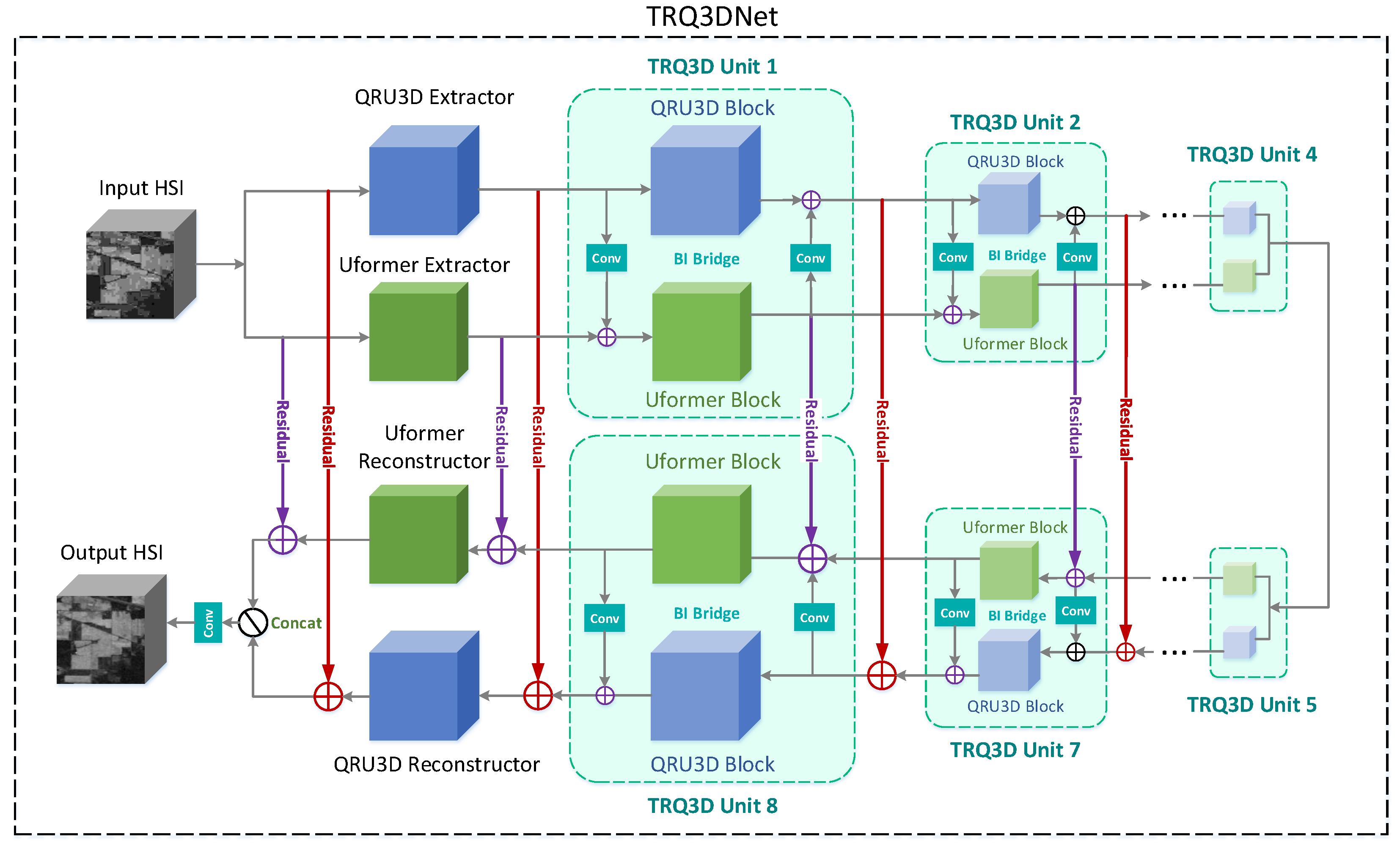
  • We propose TRQ3DNet, a residual encoder–decoder network for HSI denoising, which consists of two branches. One is based on convolution, and the other is transformer. The model can extract both the global correlation along spectrum and the local–global spatial features.
  • We present a bidirectional integration bridge, which aggregates the global features from convolution layers and the local features from window-based attention mechanism, so as to exploit a better representation of image features.
  • We conduct both synthetic and real HSI denoising experiments. Quantitative evaluation results reveal that our model achieves a better performance than other state-of-the-art model-based and deep-learning-based methods.
The rest of the paper is organized as follows: We introduce the proposed method in Section 2, and the experimental results are presented in Section 3. In Section 4, we conduct analysis and discussion, and in Section 5 we draw the conclusion. Code is available at https://github.com/LiPang/TRQ3DNet (on 8 September 2022).

2. Proposed Method

2.1. Notations

An HSI Y degraded by various noise can be described as a linear model:
Y = X + N ,
where X is the ideal noise-free image, and N is the addictive noise, e.g., Gaussian noise. Y , X , N R B × H × W , and H, W, B represent the height, the width, and the band number of the HSI, respectively. The goal of HSI denoising is to recover the clean X from the noisy observation Y .

2.2. Overall Architecture

The overall architecture of the TRQ3DNet is shown in Figure 1. Our network consists of an extractor, a reconstructor, and four pairs of symmetric TRQ3D units. The basic unit of the residual encoder–decoder network consists of three parts: 3D quasi-recurrent block (QRU3D block), Uformer block, and the bidirectional integration bridge (BI bridge).
The input degraded HSIs X are fed into the QRU3D and Uformer extractors separately to extract low-level features. As for the QRU3D extractor, the input firstly goes through a bidirectional QRU3D layer and obtains output named X q r u . For the Uformer extractor, the input is applied with a dimensional transformation (2D convolution with LeakyReLU [38] activation) and obtains X t r a n s . Next, X q r u and X t r a n s are fed into a sequence of TRQ3D units which are composed of QRU3D and Uformer blocks. Before X t r a n s is input into the Uformer block, information from the QRU3D block is integrated. We apply a 3D and 2D convolution to X q r u , which has the same dimensions as X t r a n s by setting the proper stride of the convolution kernel, then the weighted element-wise sum of the two parts are fed into the Uformer block, and we obtain the output. This output serves as the input for the next Uformer block. At the same time, the original X q r u goes through the QRU3D block, and is added to the output from Uformer block (we also perform the weighted element-wise sum), which is the input of the next QRU3D block. Eventually, the restored image is obtained via QRU3D and Uformer reconstructors which are structured similarly to extractors. Above all, the degraded HSIs are passed into extractors to extract low-level characteristics. After being processed by a succession of TRQ3D units, clean HSIs are obtained by reconstructors. Each TRQ3D unit takes two results from the previous unit as inputs, one from the QRU3D block and the other from the Uformer block. The two inputs are separately fed into the two blocks with information exchange, which generates two outputs that are fed into the next TRQ3D unit.
We set stride = 2 of 3D convolution for the first half of the blocks, and stride = 1/2 for the rest, separately. By adapting the stride of the convolution kernel, we can perform downsampling operations in the encoder part and upsampling operations in the decoder part. This can lessen the computation cost, reduce the risk of overfitting, and make the network more adaptable to larger datasets. In the following, we introduce the three components of the network in detail.

2.3. 3D Quasi-Recurrent Block

As seen in Figure 2, the 3D quasi-recurrent (QRU3D) block is one of the components of the TRQ3D unit, which is composed of two modules: a 3D convolution module and a quasi-recurrent pooling module.
(1)
3D Convolution Module: We apply two sets of 3D convolution [39,40] to the inputs, which activates the convolution output with two different nonlinear functions, and generates two tensors, named candidate tensor Z and forget gate tensor F . The process is formulated as
Z = σ ( W Z X ) ,
F = s i g m o i d ( W F X ) ,
where X R C i n × B × H × W is the input feature map from the last layer, and C i n is the number of input channels. σ represents a certain activation function, e.g., tanh, relu or without activation. { Z , F } R C o u t × B × H × W and C o u t are the number of output channels. { W Z , W F } R C o u t × C i n × 3 × 3 × 3 are 3D convolution kernels. Notice that we only use sigmoid for gate tensor F, in order to map the output to values between 0 and 1. Compared with 2D convolution, 3D convolution can not only aggregate spatial domain information, but also exploit the spectral information of the input.
(2)
Quasi-Recurrent Pooling Module: Considering that the 3D convolution can only aggregate the information in adjacent bands, motivated by the QRNN3D [22], we introduce the quasi-recurrent pooling operation and dynamic gating mechanism in order to fully exploit global correlation along all the bands. We split the candidate tensor and forget gate tensor along the spectrum direction, obtaining sequences Z = { z 1 , z 2 , , z B } and F = { f 1 , f 2 , , f B } . Then, these sequences are applied with the quasi-recurrent pooling operation, as shown below:
h i = f i h i 1 + ( 1 f i ) z i , i = 1 , 2 , , B ,
where h i is the i-th hidden state ( h 0 = 0 ), and ⊙ represents the Hadamard product. The value of f i controls the weight of candidate tensor z i and states from the last step h i 1 . The sigmoid is used as the activation function for the forget gate. All h i are concatenated along the spectral dimension, generating the output. The benefits of quasi-recurrent pooling are that the module will automatically preserve the information of each spectrum z i through the training process, and achieve global correlation along all spectra. Notice that the hidden state only depends on the current band of the input feature map, so the gate tensor relies more on the input as well as the parameters learned from the training process.

2.4. Uformer Block

As is shown in Figure 3, each Uformer block is stacked by two LeWin transformer blocks [37]. Each LeWin transformer block has two basic modules: window-based multi-head self-attention (W-MSA) and locally-enhanced feed-forward network (LeFF), which are described as
X ^ ( l ) = W - MSA ( LN ( X ( l 1 ) ) ) + X ( l 1 ) ,
X ( l ) = LeFF ( X ^ ( l ) ) + X ^ ( l ) ,
where X ^ ( l ) and X ( l ) represent the output feature maps of the l-th W-MSA and LeFF module. LN represents the layer normalization [41].
(1)
Window-based Multi-head Self-Attention: The projection layer transforms the bands value of the input feature maps, from X R B × H × W to X R B o u t × H × W . Each band of the feature maps is seen as a 2D map, which is partitioned into non-overlapping windows with size M × M , expressed as X = { X 1 , X 2 , . . . , X N } , where N = H W / M 2 is the number of windows (also called patches), and X i R B o u t × M × M , i = 1 , 2 , . . . , N . Then, we flatten these image patches with size M 2 × B o u t , and calculate the multi-head self-attention on each of them. Given the total number of head K, we can draw that the dimension of k-th head is D k = B o u t / K , and the k-th self-attention of X i is calculated as
Y i ( k ) = A t t e n t i o n ( X i W Q ( k ) , X i W K ( k ) , X i W V ( k ) ) ,
where { W Q ( k ) , W K ( k ) , W V ( k ) } R B o u t × D k are learnable weight matrices. When calculating the self-attention, we also employ the relative position bias B R M 2 × M 2 to each head, following the work of [37]. Thus, the attention mechanism is
A t t e n t i o n ( Q , K , V ) = S o f t M a x ( Q K T D k + B ) V ,
and Q , K , V represent the query, key, and value, separately. The values in B are taken from a smaller bias matrix B ^ R ( 2 M 1 ) × ( 2 M 1 ) with learnable parameter [42,43]. For N patches X i R M 2 × B o u t , i = 1 , 2 , . . . , N , we obtain corresponding N output feature maps Y i ( k ) R M 2 × D K of k-th head, described as Y ( k ) = { Y 1 ( k ) , Y 2 ( k ) , . . . , Y N ( k ) } R N × M 2 × D K in a whole. Finally, outputs of K heads are concatenated together followed by a linear transform to generate the result of the LeWin transformer block.
(2)
Locally-enhanced Feed-Forward Network: The feed-forward network (FFN) in the standard transformer model provides linear dimensional transformation and nonlinear activation to the tokens from the W-MSA module, which enhances the ability of feature representation. The limitation is that the spatial correlation among neighboring pixels is ignored. To overcome this problem, we replace the FFN with a locally-enhanced feed-forward network (LeFF), because the latter model provides depth-wise convolution to extract the spatial information. The process is as follows. First, the input feature maps are fed into a linear layer, and projected to a higher dimension. Next, we reshape the feature maps to 2D feature, using a 3 × 3 depth-wise convolution to capture local information. Then, we flatten back the features and shrink the channels via another linear layer to match the dimension of the input channels. For each linear and convolution layer, GELU [44] is used as the activation function since it has been proven to achieve comparable denoising results compared with other activation functions [36,37].

2.5. Bidirectional Integration Bridge

We propose a bidirectional integration bridge (BI bridge), to combine and enhance the representation of image features. The 3D convolution extracts the local spatial correlation and spectral correlation between neighboring bands. The quasi-recurrent pooling exploits the global correlation along the spectrum. The Uformer block is able to exploit the global spatial features. The BI bridge is used to combine the three parts to better preserve image details. We point out that the size of the QRU3D output feature map is C q r u × B × H × W , while the Uformer output is C t r a n s × H × W .
On one hand, the input of the next Uformer layer is the weighted sum of outputs of the current Uformer layer and the QRU3D layer. In order to match the output size from the two modules, dimensional transformation is necessary. We first conduct a 3D convolution operation, shaping the feature map from C q r u × B × H × W to 1 × B × H × W , and squeeze it to B × H × W . Then, the feature map is applied with a 2D convolution, transforming from B × H × W to C t r a n s × H × W . Finally, the element-wise sum of this feature map and the Uformer layer output is the input of the next Uformer layer. This dimension transformation, making the QRU3D feature map adapt to the Uformer block, is seen as a unidirectional bridge.
On the other hand, the input of the next QRU3D layer is also the weighted sum of outputs of the current Uformer layer and the QRU3D layer. We use the reverse transformation method above. Firstly, a 2D convolution transforms the Uformer layer output with size C t r a n s × H × W to size B × H × W . Then, we unsqueeze it to 1 × B × H × W , and apply a 3D convolution to size C q r u × B × H × W . Finally, we perform a 1 × 1 × 1 3D convolution operation on the element-wise sum of this feature map and the QRU3D layer output, generating the input of the next QRU3D layer. This dimension transformation, making the Uformer feature map adapt to the QRU3D block, is the other directional integration bridge. Essentially, the BI bridge is made up of two directional (from QRU3D to Uformer, and reverse) dimension transformations, based on 2D and 3D convolution.

2.6. Training Loss Function

In this part, we introduce the loss function used in the training process. The l 1 loss and l 2 loss are often used in order to make a balance between noise removal and detail preservation [23]. In this paper, we adopt the l 2 loss as the final loss function, which is defined as
L = 1 N i = 1 N | | X i X i ( g t ) | | 2 ,
where N is the number of training patch image, and X i and X i ( g t ) represent the output denoised image patch and ground truth image patch, respectively.

3. Experiments

3.1. Experimental Setup

In this section, we conduct several experiments to evaluate the model. In the following, we introduce the datasets we use, the denoising methods to compete with, and training strategies, as well as evaluation metrics. Code is available at https://github.com/LiPang/TRQ3DNet (on 8 September 2022).
Dataset: We conduct synthetic experiments on the ICVL dataset [45], CAVE [46], Pavia Centre [47] and Pavia University [47], in which the HSIs can be seen as clean. In addition, real HSI denoising experiments are conducted on real remotely sensed hyperspectral datasets, e.g., Urban [48] and Indian Pines [49]. The overall information of the involved datasets can be seen in Table 1.
The ICVL dataset, which contains 201 images, is randomly divided into three disjointed parts for training, validation, and testing. Taking the training time into account, we use 100 images to train, 20 images to validate, and the rest to test our model. To enlarge the training dataset, we crop the images into multiple overlapped cubes with size 64 × 64 and bands 31 (same as the original bands number) to preserve the spectral domain integrity. In addition, transformations such as rotation and scalings are adopted, and we thus generate about 50 k training HSIs patches in total. As for testing and validation, the images are cropped to 512 × 512 × 31 from their domain region. To better assess the robustness of the trained model, in addition to 20 samples from ICVL dataset, we select 10 samples from CAVE, adding various noises (e.g., Gauss, impulse, mixture) as the validation set.
The CAVE dataset is made up of 31 hyperspectral images at a spatial size of 512 × 512 with 31 bands. To better evaluate the performance of different models, we perform threefold cross validation on the CAVE dataset. We use 21 images for training and the remaining 11 images for testing in each fold. Similar to the process procedure of the ICVL training set, we crop the training images into cubes with size 64 × 64 and bands 31, and perform rotation and scalings transformations, generating 2562 training patches.
Remotely sensed hyperspectral datasets (i.e., Pavia Centre, Pavia University, Indian Pines, and Urban) are used to further verify the stability and adaptability of our model. The number of spectral bands of Pavia Centre is 102 and that of Pavia University is 103, and both datasets were captured by the ROSIS sensor. Indian Pines and Urban were obtained using the 224-bands AVIRIS sensor and 210-bands HYDICE hyperspectral system, respectively.
Competing Methods: We conduct synthetic experiments as well as real HSIs denoising experiments. In both sets of experiments, several state-of-the-art model-based methods and deep-learning-based models are compared.
To evaluate the HSI denoising method, two types of synthetic experiments are often needed. The first one is the Gaussian noise experiment, and the second one is the complex noise case. For each of the two cases, the state-of-the-art (SOTA) methods are quite different, which has been recognized by existing work [22]. Therefore, in our experiments, we use different SOTA methods for the two cases. In synthetic experiments, we compare our method with the model-based methods (BM4D [11], TDL [10], ITSReg [12], LLRT [13]), and the deep-learning-based methods (HSID-CNN [20], swinir [36], QRNN3D [22]) in Gaussian noise case, and model-based methods (LRMR [14], LRTV [15], NMoG [16], and TDTV [17]), and the same deep-learning-based methods in complex noise case. All approaches based on deep learning are trained and tested in the same condition to ensure fairness.
Network Training: The training process contains three successive stages with increasing difficulty, from Gaussian noise with certain intensity to uncertain case, from single noise to mixture case. The model is trained by minimizing the mean square error (MSE) between degraded HSIs and the corresponding ground truth. The parameters are optimized by Adam optimizer [50]. The whole project is based on the deep learning framework Pytorch on a machine with Tesla V100 PCIe GPU, Intel(R) Xeon(R) CPU E5-2690 v4 of 2.60 GHz and 503 GB RAM.
Evaluation Metrics: We adopt three common metrics to evaluate the performance of the models in the synthetic experiment, including PSNR, SSIM [51], and SAM [52], and report the time cost for each model. The first two metrics measure the spatial similarity, and the last measures the spectral similarity. Given a reference image I and the reconstruction image I ^ , PSNR can be calculated as
PSNR = 10 l o g 10 ( 2 n 1 ) 2 M S E
MSE = 1 H W i = 1 H j = 1 W [ I ( i , j ) I ^ ( i , j ) ] 2
where H and W represent the height and width of the image, and n is the pixel digits which is usually 8. The core formula of SSIM can be shown as follows:
SSIM = ( 2 μ I μ I ^ + c 1 ) ( 2 σ I I ^ + c 2 ) ( μ I 2 + μ I ^ 2 + c 1 ) ( σ I 2 + σ I ^ 2 + c 2 )
where μ I and μ I ^ are the mean values of images I and I ^ , σ I 2 and σ I ^ 2 are the respective variances of images I and I ^ , and σ I I ^ is the covariance of the images I and I ^ . The higher the PSNR and SSIM, and the lower the SAM, the better the model performs. Furthermore, we adopt a no-reference quality assessment proposed by Liu et al [53] for HSI denoising, which evaluates the image quality according to the changes in kurtosis values of noisy images. The lower the score, the higher the quality of the recovered image. As HSIs contain hundreds of bands, we calculate PSNR, SSIM, and the no-reference quality score for each band of the HSIs, and take the average value as the final result.

3.2. Synthetic Experiments

In synthetic experiments, we simulate the real situation by adding various noise to HSIs artificially. Many experimental works for the HSI denoising task assume that the HSIs are usually contaminated by Gaussian, impulse, dead pixels, lines, and stripes noises [54]. Therefore, we design five noise combinations, as shown below:
Case 1: Non-i.i.d. Gaussian Noise. Gaussian noise with zero mean, as well as intensities randomly set from 10 to 70, is added to each band.
Case 2: Gaussian + Stripe Noise. On the basis of Case 1, all bands have Gaussian noise added, among which 10 bands are randomly selected to be corrupted by stripe noise. The number of stripes in each band is 5% to 15% of the number of columns by uniform sampling.
Case 3: Gaussian + Deadline Noise. Similar to Case 2, the only difference is that we use deadline noise instead of stripe noise.
Case 4: Gaussian + Impulse Noise. On the basis of Case 1, all bands have Gaussian noise added, among which 10 bands are randomly selected to be corrupted by impulse noise, and the intensity of impulse noise ranges from 10% to 70% by uniform sampling.
Case 5: Mixture Noise. On the basis of Case 1, all bands have Gaussian noise added, among which 10 bands are randomly selected to be corrupted by one of the extra noise mentioned in above cases.
We adapt the training and testing strategy mentioned above (see experimental setup). Specifically, in stage 1, namely, in the first 30 epochs, the training set is formed by HSIs corrupted by Gaussian noise with zero mean and known noise intensity σ = 50 , and batch size set to 16. In stage 2, from epochs 30 to 50, it is similar to stage 1, yet the intensity of Gaussian noise is uniformly sampled from 30 to 70. In stage 3, from epochs 50 to 100, we use noise combinations randomly chosen from Case 1 to Case 4. Batch size in stage 2 and 3 is set to 64 to stabilize the training process. At the end of stages 2 and 3, we test the model on the Gaussian denoising task and complex denoising task separately.
Gaussian Noise Denoising on ICVL: We compare our model with four model-based methods (BM4D, TDL, ITSReg, and LLRT) and three DL-based methods (HSID-CNN, swinir, and QRNN3D). Figure 4 presents the Gaussian denoising example (with noise intensity σ = 50 ) of the ICVL dataset. Intuitively, we evaluate the performance of the model on different levels of Gaussian noise intensity ( σ = 30 , 50 , 70 and blind). The qualitative evaluation results and time cost are shown in Table 2. Compared with other methods, our model achieves better performances in most Gaussian noise cases.
Complex Noise Denoising on ICVL: We compare our model with four model-based methods (LRMR, LRTV, NMoG, and LRTDTV) and three DL-based methods (HSID- CNN [20], swinir [36], and QRNN3D [22]). We evaluate the performance of the model in complex noise cases from Case 1 to Case 5 mentioned above, select one of the images from each case, and visualize the restoration status in Figure 5. The qualitative evaluation results and time cost are shown in Table 3. The results show that our model outperforms other state-of-the-art methods in all cases. We plot the PSNR value of each band in Gaussian and complex noise cases, as seen in Figure 6. We can easily observe that the PSNR values of most bands obtained by our model are higher than competing methods, indicating that our model outperforms others.
Complex Noise Denoising on CAVE: In addition to testing on ICVL, we also perform threefold cross validation on the CAVE dataset in the mixture noise case. Since the CAVE dataset is small, which is prone to cause overfitting, we employ a small amount of samples from the CAVE dataset to fine-tune the model trained on the ICVL dataset instead of training from scratch. All the competing DL-based approaches are trained in the same way for fair comparison. The experimental results are shown in Table 4, from which we can observe that our proposed TRQ3DNet obtains the best denoising performance compared with other methods.
Complex Noise Denoising on Pavia University: To further verify the effectiveness of our proposed method, we also conduct experiments on the Pavia University dataset in the mixture noise case. Considering the similarity between Pavia Centre and Pavia University, we first evaluate the performance of our method trained from scratch on Pavia Centre (denoted as Ours-S). The Ours-S model seems to overfit the data and obtains an undesirable result owing to the fact that the Pavia Centre training set is relatively small (only 969 patches of size 64 × 64 × 31 , which is small compared with 53,000 training patches of the ICVL dataset). Nevertheless, the model trained on the ICVL dataset (denoted as Ours-P) outperforms all the other methods. For fair comparison, all the DL-based methods are obtained by the model trained on the ICVL dataset, which is the same as Ours-P. Furthermore, we fine-tuned the Ours-P model for another 50 epochs on the Pavia Centre dataset (denoted as Ours-F). It can be observed from Table 5 that the fine-tuned model significantly boosts the performance, which verifies the adaptability of our proposed TRQ3DNet.

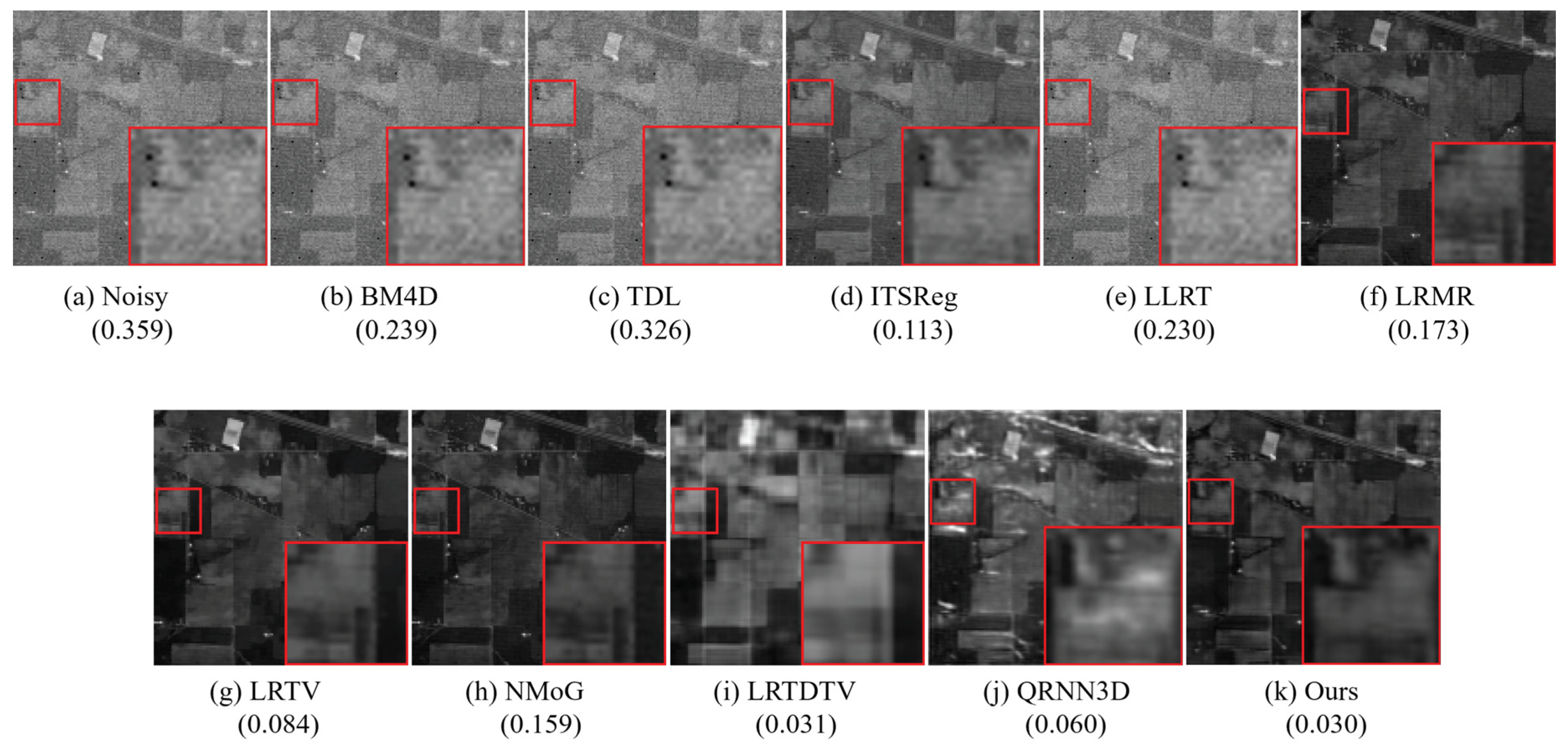
3.3. Real HSI Denoising

Except for the aforementioned synthetic experiments, we also evaluate our model on two real HSI datasets, i.e., Indian Pines and Urban. The two real noisy HSI datasets have no ground truth image for reference, and thus it is very difficult to evaluate the performance. In this paper, we adopt the visualization and one no-reference quality assessment proposed in [53] for HSI denoising, which evaluates the image quality according to the changes in kurtosis values of noisy images. The lower the score, the higher the quality of the recovered image. As illustrated in Table 6, TRQ3DNet achieves the best denoising performance in terms of this index. Additionally, we also show some visualization comparison results in Figure 7 and Figure 8, from which it can be seen that our model achieves better performance than other methods since it can not only remove the complex noise, but also preserve the local details of the HSIs, which is consistent with the quantitative results.

3.4. Ablation Study

Our model has three main components: QRU3D block, Uformer block, and BI bridge. To explore the specific function of each part, we design the following ablation experiments. We follow the steps in Section 5, and test different noise combinations from Case 1 to Case 5. Results from swinir and QRNN3D are listed as reference. Our QRU3D block has a slight difference from that in QRNN3D, where our model contains 1 × 1 convolution layers, when fusing the output from two blocks.
Investigations of Subcomponent: We split our model into three parts (QRU3D block, Uformer block, and BI bridge) and test each part independently, which are recorded as QRU3D, TR, and WithoutI, separately. WithoutI is the combination of the QRU3D block and the Uformer block with the BI bridge removed, and the purpose is to explore the improvement of the BI bridge to the model.
QRU3D Block: To investigate the role of QRU3D, we remove this structure as well as the BI bridge, keeping the Uformer block only. The quantitative comparison between TR and WithoutI shows the promotion of the Uformer block on the model. Nevertheless, the parameters of the model are also greatly reduced; thus, we change the hidden channels of TR (16 to 32), called WTR, with approximate parameters with the full model. The results show that WithoutI outperforms the TR and WTR in all cases, and only the SAM value in Case 5 is larger than WTR, indicating that the QRU3D block takes positive effect and extracts features successfully. One possible reason why TR performs poorly is that, different from the image classification task in which general information is more important, the image denoising problem focuses more on the details of the image, such as the value of each pixel. Compared with transformer, convolutional neural network can better capture the local correlation and preserve image details [55], and thus obtain better denoising performance.
Uformer Block: Similar to the first experiment, we keep the QRU3D block and compare the performance with WithoutI. We also test WQRU3D by doubling the channels. It can be observed that the Uformer block boosts the performance to some extent.
BI Bridge: We compare the effectiveness of the original model and WithoutI (called Ours). It can be seen that Ours is the best of the bunch, demonstrating that the information interaction between the QRU3D modules and the Uformer modules can also improve the performance.
The ablation results on each sub component are listed in Table 7.
Investigations of Network Hyperparameters: The purpose of this experiment is to select hyperparameters beforehand, so as to achieve the trade-off between performance and computation cost. We consider two kinds of parameters: the depth of the model (the total number of TRQ3D blocks), and width of the model (hidden channels). We search the parameter in a small grid map on Gaussian denoising case ( σ = 50 ), and choose by the integration of PSNR value, time cost (seconds), and the size of the network. The first step is to fix width and search for the best depth, then use the best depth and determine the width. The evaluation results of each hyperparameter pair are shown in Table 8. We finally take depth = 8 and width = 16 , and apply this to the above experiments. Although the model with width = 20 achieves better results than that with width = 16 , the computation load and the network size in this case increase greatly.

4. Analysis and Discussion

4.1. Training Strategy

We adopt a three-stage training strategy in our experiment, which is an incremental training policy and has already been used to train the deep neural network to prevent the network from converging to a poor local minimum [22]. All the other DL-based models are trained in the same way so that they can be fairly compared. We also trained our proposed TRQ3DNet only using the complex noise case. As shown in Figure 9, in contrast to training incrementally, training from scratch makes the optimization converge to a poor local optimum.

4.2. Feature Analysis

We also visualized the feature maps to explicitly show the better feature preservation ability of the BI bridge. Specifically, we made comparisons of the feature maps of the second encoder layer and the third decoder layer in Figure 10. Our QRU3D and our Uformer denote the outputs of the TRQ3D block, while QRU3D and Uformer represent the feature maps of the single branch trained without other subcomponents of TRQ3DNet. It was introduced that TRQ3DNet takes advantage of both local and global features. From Figure 10, we can see that QRU3D enhances local details such as the small bright regions in the middle of the peppers. Our QRU3D benefits from the global representation of the Uformer branch and activates more decentralized areas. For example, QRU3D activates a distinct area inside the peppers in the feature map (e), while our QRU3D activates the entire peppers in the feature map (f). Compared with Uformer, our Uformer retains the detail of the local features from the QRU3D branch (e.g., (c,d)). In addition, it seems that there are obvious striping artifacts in the features. One possible reason is that the training set has stripe noise added, as described in Section 3.2, and thus the proposed network can learn the stripe features which are reflected in the outputs of the hidden layer. Therefore, even if the testing data do not contain such stripe noise, we can not guarantee whether this phenomenon will occur or not. More effective training methods can be explored to alleviate the problem.

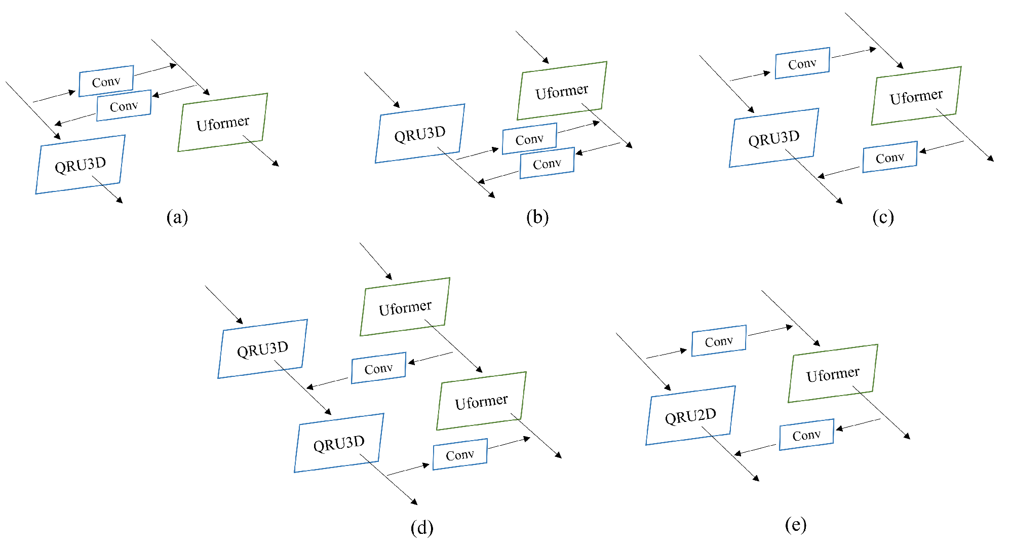
4.3. Structure Analysis

We propose the bidirectional integration bridge (BI bridge) to fuse convolutional local features with transformer-based global representations in an interactive fashion. Considering the BI bridge as a short connection, it can thus be flexibly placed in different positions of the TRQ3D unit. For example, as shown in Figure 11, case (a) and case (b) place the BI bridge in the input and the output of the unit, respectively, and case (c) places one direction of the bridge in the input and the other direction in the output. Case (a), in which the BI bridge is added before each TRQ3D unit, means that the outputs from the previous layer are firstly processed by the BI bridge (as introduced in Section 2.5) and then are fed into the Uformer and QRU3D blocks separately, generating the inputs of the next layer. Similarly, we add the BI bridges after and at both ends of each TRQ3D unit in case (b) and case (c). Furthermore, we compare the results of using a one-way bridge which means that there is only one direction of information exchange in each TRQ3D unit in case (d). In other words, only the QRU3D output or the Uformer output is added to the output of the other block (as shown in Figure 11d). In addition, we replace the 3D convolution in each TRQ3D unit with 2D convolution which is implemented by changing the convolution kernel size to 3 × 3 × 1 in case (e). Table 9 shows the denoising performance on ICVL of different network structures in the case of Gaussian noise. Although there is no significant difference, one can see that the network structure in case (c) obtains the best denoising performance. Additionally, we can empirically observe that case (c) outperforms case (a) and case (b), which may be attributed to the placement of the BI bridge in the network structure. Additionally, the one information exchange direction in case (d) leads to less computation cost but worse denoising performance as the dependency of the QRU3D and Uformer blocks is poorly modeled. The result of case (e) indicates that 3D convolution can better model spectral domain knowledge, as the spectral distortion is relieved compared to 2D convolution, which is also proved in previous work [22].

4.4. Practical Implications

HSIs are widely employed to recognize various objects and terrain land cover classes based on spectral features [56]. However, owing to environmental factors and precision of instrument, HSIs are inevitably corrupted by various noise, making model training and prediction more challenging. Therefore, to further verify the significance of our work, we compared classification performance on Pavia University and Indian Pines with different noise level. Each dataset has mixture noise added and is denoised by several methods. We train the classification network proposed in [56] for 15 epochs on each dataset under different noise situations. The network employs convolutional blocks to learn spectral and spatial characteristics and a multilayer perceptron to predict labels. Seventy-five percent of pixels are used as the training set and the rest are the testing set. For equality, the split of training and testing sets as well as parameter settings are kept the same in all cases. The results are shown in Table 10. From this table, we can observe that noisy images degrade the classification performance. In contrast, the accuracy improves significantly when denoising is performed, and our method achieves the most significant classification results improvement, even better than training with original clean images, which demonstrates the value of our work.

4.5. Limitations Analysis

Although our network achieves excellent denoising performance, there are still several limitations. Firstly, since the TRQ3D unit is composed of two blocks (i.e., QRU3D and Uformer), more computational cost is required. One of our future research directions focuses on modifying the network structure to be lighter so that the performance can still be preserved while the running time can be reduced. Secondly, the BI bridge is composed of 2D and 3D convolutional blocks, leading to a sharp increase in parameters and computation cost when the number of hidden layer channels is large. As a consequence, it is possible to investigate more efficient aggregation methods. Last, but not least, similar to most deep-learning-based methods, TRQ3DNet can be well trained and tested on a single dataset, while the denoising performance of the model dramatically degrades in a new dataset. In the future, we will focus on this generalization issue and try to alleviate this limitation.

5. Conclusions and Future Work

In this paper, we design a new network (i.e., TRQ3DNet) for HSI denoising. This network is composed of two branches. The first one is based on the 3D quasi-recurrent block, including convolution and quasi-recurrent pooling operation, and can help to extract the local spatial correlation and the global correlation along the spectrum. The second branch contains the Uformer block with window-based multi-head self-attention (W-MSA) and locally-enhanced feed-forward network (LeFF) to exploit the global spatial features. Experimental results on synthetic and real HSI denoising illustrate the superiority of our proposed network compared with other state-of-the-art methods.
Specifically, in the future work, it is worth investigating a more effective training strategy in case the performance on previous datasets degrades when training on a new dataset. In addition, the structure of the network and the aggregation methods can be further exploited to lighten the model so that the running time can be reduced. In addition, more real HSI datasets can be used for training to improve the model performance. In addition, better validation methods should be considered to verify the effectiveness of the proposed network.

Author Contributions

Formal analysis, L.P.; funding acquisition, X.C.; methodology, L.P.; project administration, W.G.; writing—original draft, W.G.; writing—review and editing, X.C. All authors have read and agreed to the published version of the manuscript.

Funding

This work was supported by National Key Research and Development Project of China (2021ZD0110700), National Natural Science Foundation of China (62272375, 61906151, 62050194, 62037001), Innovative Research Group of the National Natural Science Foundation of China(61721002), Innovation Research Team of Ministry of Education (IRT_17R86), Project of China Knowledge Centre for Engineering Science and Technology, and Project of XJTU Undergraduate Teaching Reform (20JX04Y).

Data Availability Statement

The datasets generated during the study are available from the corresponding author on reasonable request.

Conflicts of Interest

The authors declare no conflict of interest.

References

  1. Akhtar, N.; Mian, A. Nonparametric coupled bayesian dictionary and classifier learning for hyperspectral classification. Neural Netw. Learn. Syst. IEEE Trans. 2018, 29, 4038–4050. [Google Scholar] [CrossRef] [PubMed]
  2. Camps-Valls, G.; Tuia, D.; Bruzzone, L.; Benediktsson, J.A. Advances in hyperspectral image classification: Earth monitoring with statistical learning methods. IEEE Signal Process. Mag. 2013, 31, 45–54. [Google Scholar] [CrossRef]
  3. Zhong, P.; Wang, R. Jointly learning the hybrid crf and mlr model for simultaneous denoising and classification of hyperspectral imagery. IEEE Trans. Neural Netw. Learn. Syst. 2014, 25, 1319–1334. [Google Scholar] [CrossRef]
  4. Wang, Q.; Lin, J.; Yuan, Y. Salient band selection for hyperspectral image classification via manifold ranking. IEEE Trans. Neural Netw. Learn. Syst. 2017, 27, 1279–1289. [Google Scholar] [CrossRef]
  5. Yang, S.; Feng, Z.; Min, W.; Kai, Z. Self-paced learning-based probability subspace projection for hyperspectral image classification. IEEE Trans. Neural Netw. Learn. Syst. 2019, 30, 630–635. [Google Scholar] [CrossRef]
  6. Ayerdi, B.; Marques, I.; Grana, M. Spatially regularized semisupervised ensembles of extreme learning machines for hyperspectral image segmentation. Neurocomputing 2015, 149, 373–386. [Google Scholar] [CrossRef]
  7. Noyel, G.; Angulo, J.; Jeulin, D. On distances, paths and connections for hyperspectral image segmentation. arXiv 2016, arXiv:1603.08497. [Google Scholar]
  8. Li, J.; Agathos, A.; Zaharie, D.; Bioucas-Dias, J.M.; Plaza, A.; Li, X. Minimum volume simplex analysis: A fast algorithm for linear hyperspectral unmixing. IEEE Trans. Geosci. Remote Sens. 2015, 53, 5067–5082. [Google Scholar]
  9. Rasti, B.; Chang, Y.; Dalsasso, E.; Denis, L.; Ghamisi, P. Image restoration for remote sensing: Overview and toolbox. arXiv 2021, arXiv:2107.00557. [Google Scholar] [CrossRef]
  10. Peng, Y.; Meng, D.; Xu, Z.; Gao, C.; Yang, Y.; Zhang, B. Decomposable nonlocal tensor dictionary learning for multispectral image denoising. In Proceedings of the IEEE Conference on Computer Vision and Pattern Recognition, Columbus, OH, USA, 23–28 June 2014; pp. 2949–2956. [Google Scholar]
  11. Maggioni, M.; Katkovnik, V.; Egiazarian, K.; Foi, A. Nonlocal transform-domain filter for volumetric data denoising and reconstruction. IEEE Trans. Image Process. 2012, 22, 119–133. [Google Scholar] [CrossRef]
  12. Xie, Q.; Zhao, Q.; Meng, D.; Xu, Z.; Gu, S.; Zuo, W.; Zhang, L. Multispectral images denoising by intrinsic tensor sparsity regularization. In Proceedings of the IEEE Conference on Computer Vision and Pattern Recognition, Las Vegas, NV, USA, 27–30 June 2016; pp. 1692–1700. [Google Scholar]
  13. Chang, Y.; Yan, L.; Zhong, S. Hyper-laplacian regularized unidirectional low-rank tensor recovery for multispectral image denoising. In Proceedings of the IEEE Conference on Computer Vision and Pattern Recognition, Honolulu, HI, USA, 21–26 July 2017; pp. 4260–4268. [Google Scholar]
  14. Zhang, H.; He, W.; Zhang, L.; Shen, H.; Yuan, Q. Hyperspectral image restoration using low-rank matrix recovery. IEEE Trans. Geosci. Remote Sens. 2013, 52, 4729–4743. [Google Scholar] [CrossRef]
  15. He, W.; Zhang, H.; Zhang, L.; Shen, H. Total-variation-regularized low-rank matrix factorization for hyperspectral image restoration. IEEE Trans. Geosci. Remote Sens. 2015, 54, 178–188. [Google Scholar] [CrossRef]
  16. Chen, Y.; Cao, X.; Zhao, Q.; Meng, D.; Xu, Z. Denoising hyperspectral image with non-iid noise structure. IEEE Trans. Cybern. 2017, 48, 1054–1066. [Google Scholar] [CrossRef]
  17. Wang, Y.; Peng, J.; Zhao, Q.; Leung, Y.; Zhao, X.; Meng, D. Hyperspectral image restoration via total variation regularized low-rank tensor decomposition. IEEE J. Sel. Top. Appl. Earth Obs. Remote Sens. 2017, 11, 1227–1243. [Google Scholar] [CrossRef]
  18. Dabov, K.; Foi, A.; Katkovnik, V.; Egiazarian, K. Image denoising by sparse 3-d transform-domain collaborative filtering. IEEE Trans. Image Process. 2007, 16, 2080–2095. [Google Scholar] [CrossRef]
  19. Chang, Y.; Yan, L.; Fang, H.; Zhong, S.; Liao, W. Hsi-denet: Hyperspectral image restoration via convolutional neural network. IEEE Trans. Geosci. Remote Sens. 2018, 57, 667–682. [Google Scholar] [CrossRef]
  20. Yuan, Q.; Zhang, Q.; Li, J.; Shen, H.; Zhang, L. Hyperspectral image denoising employing a spatial-spectral deep residual convolutional neural network. IEEE Trans. Geosci. Remote Sens. 2018, 57, 1205–1218. [Google Scholar] [CrossRef]
  21. Tai, Y.; Yang, J.; Liu, X.; Xu, C. Memnet: A persistent memory network for image restoration. In Proceedings of the 2017 IEEE International Conference on Computer Vision (ICCV), Venice, Italy, 22–29 October 2017; pp. 4549–4557. [Google Scholar]
  22. Wei, K.; Fu, Y.; Huang, H. 3-d quasi-recurrent neural network for hyperspectral image denoising. IEEE Trans. Neural Netw. Learn. Syst. 2020, 32, 363–375. [Google Scholar] [CrossRef]
  23. Cao, X.; Fu, X.; Xu, C.; Meng, D. Deep spatial-spectral global reasoning network for hyperspectral image denoising. IEEE Trans. Geosci. Remote Sens. 2021, 60, 1–14. [Google Scholar] [CrossRef]
  24. He, K.; Zhang, X.; Ren, S.; Sun, J. Deep residual learning for image recognition. In Proceedings of the IEEE Conference on Computer Vision and Pattern Recognition, Las Vegas, NV, USA, 26 June–1 July 2016; pp. 770–778. [Google Scholar]
  25. Vaswani, A.; Shazeer, N.; Parmar, N.; Uszkoreit, J.; Jones, L.; Gomez, A.N.; Kaiser, L.; Polosukhin, I. Attention is all you need. Adv. Neural Inf. Process. Syst. 2017, 30. [Google Scholar]
  26. Heo, B.; Yun, S.; Han, D.; Chun, S.; Choe, J.; Oh, S.J. Rethinking spatial dimensions of vision transformers. In Proceedings of the IEEE/CVF International Conference on Computer Vision, Virtual, 11–17 October 2021; pp. 11936–11945. [Google Scholar]
  27. Dosovitskiy, A.; Beyer, L.; Kolesnikov, A.; Weissenborn, D.; Houlsby, N. An image is worth 16 × 16 words: Transformers for image recognition at scale. arXiv 2020, arXiv:2010.11929. [Google Scholar]
  28. Vaswani, A.; Ramachandran, P.; Srinivas, A.; Parmar, N.; Shlens, J. Scaling local self-attention for parameter efficient visual backbones. In Proceedings of the IEEE/CVF Conference on Computer Vision and Pattern Recognition, Virtual, 11–17 October 2021; pp. 12894–12904. [Google Scholar]
  29. Maji, B.; Swain, M. Advanced fusion-based speech emotion recognition system using a dual-attention mechanism with conv-caps and bi-gru features. Electronics 2022, 11, 1328. [Google Scholar] [CrossRef]
  30. Yu, W.; Luo, M.; Zhou, P.; Si, C.; Zhou, Y.; Wang, X.; Feng, J.; Yan, S. Metaformer is actually what you need for vision. In Proceedings of the IEEE/CVF Conference on Computer Vision and Pattern Recognition, Virtual, 21–24 June 2022; pp. 10819–10829. [Google Scholar]
  31. Chu, X.; Tian, Z.; Wang, Y.; Zhang, B.; Ren, H.; Wei, X.; Xia, H.; Shen, C. Twins: Revisiting the design of spatial attention in vision transformers. Adv. Neural Inf. Process. Syst. 2021, 34, 9355–9366. [Google Scholar]
  32. Fu, J.; Liu, J.; Tian, H.; Li, Y.; Bao, Y.; Fang, Z.; Lu, H. Dual attention network for scene segmentation. In Proceedings of the 2019 IEEE/CVF Conference on Computer Vision and Pattern Recognition (CVPR), Long Beach, CA, USA, 15–20 June 2019. [Google Scholar]
  33. Jiang, Y.; Chang, S.; Wang, Z. Transgan: Two pure transformers can make one strong gan, and that can scale up. Adv. Neural Inf. Process. Syst. 2021, 34, 14745–14758. [Google Scholar]
  34. Zhao, L.; Zhang, Z.; Chen, T.; Metaxas, D.N.; Zhang, H. Improved transformer for high-resolution gans. Adv. Neural Inf. Process. Syst. 2021, 34, 18367–18380. [Google Scholar]
  35. Xu, R.; Xu, X.; Chen, K.; Zhou, B.; Chen, C.L. Stransgan: An empirical study on transformer in gans. arXiv 2021, arXiv:2110.13107. [Google Scholar]
  36. Liang, J.; Cao, J.; Sun, G.; Zhang, K.; Gool, L.V.; Timofte, R. Swinir: Image restoration using swin transformer. In Proceedings of the IEEE/CVF International Conference on Computer Vision, Virtual, 11–17 October 2021; pp. 1833–1844. [Google Scholar]
  37. Wang, Z.; Cun, X.; Bao, J.; Zhou, W.; Liu, J.; Li, H. Uformer: A general u-shaped transformer for image restoration. In Proceedings of the IEEE/CVF Conference on Computer Vision and Pattern Recognition, Seattle, WA, USA, 14–19 June 2020; pp. 17683–17693. [Google Scholar]
  38. Xu, B.; Wang, N.; Chen, T.; Li, M. Empirical evaluation of rectified activations in convolutional network. arXiv 2015, arXiv:1505.00853. [Google Scholar]
  39. Ji, S.; Xu, W.; Yang, M.; Yu, K. 3d convolutional neural networks for human action recognition. IEEE Trans. Pattern Anal. Mach. Intell. 2013, 35, 221–231. [Google Scholar] [CrossRef]
  40. Tran, D.; Bourdev, L.; Fergus, R.; Torresani, L.; Paluri, M. Learning spatiotemporal features with 3d convolutional networks. In Proceedings of the 2015 IEEE International Conference on Computer Vision (ICCV), Santiago, Chile, 7–13 December 2015; pp. 4489–4497. [Google Scholar]
  41. Ba, J.L.; Kiros, J.R.; Hinton, G.E. Layer normalization. arXiv 2016, arXiv:1607.06450. [Google Scholar]
  42. Liu, Z.; Lin, Y.; Cao, Y.; Hu, H.; Wei, Y.; Zhang, Z.; Lin, S.; Guo, B. Swin transformer: Hierarchical vision transformer using shifted windows. In Proceedings of the 2021 IEEE/CVF International Conference on Computer Vision (ICCV), Virtual, 11–17 October 2021; pp. 9992–10002. [Google Scholar]
  43. Shaw, P.; Uszkoreit, J.; Vaswani, A. Self-attention with relative position representations. arXiv 2018, arXiv:1803.02155. [Google Scholar]
  44. Hendrycks, D.; Gimpel, K. Bridging Nonlinearities and Stochastic Regularizers with Gaussian Error Linear Units. 2016. Available online: https://openreview.net/forum?id=Bk0MRI5lg (accessed on 8 September 2022).
  45. Arad, B.; Ben-Shahar, O. Sparse recovery of hyperspectral signal from natural rgb images. In Computer Vision—ECCV 2016; Leibe, B., Matas, J., Sebe, N., Welling, M., Eds.; Springer International Publishing: Cham, Switzerland, 2016; pp. 19–34. [Google Scholar]
  46. Park, J.I.; Lee, M.H.; Grossberg, M.D.; Nayar, S.K. Multispectral imaging using multiplexed illumination. In Proceedings of the IEEE International Conference on Computer Vision, Rio De Janeiro, Brazi, 14–21 October 2007. [Google Scholar]
  47. Gamba, P. A collection of data for urban area characterization. In Proceedings of the IGARSS 2004. 2004 IEEE International Geoscience and Remote Sensing Symposium, Anchorage, AK, USA, 20–24 September 2004; Volume 1, p. 72. [Google Scholar]
  48. Mnih, V.; Hinton, G.E. Learning to detect roads in high-resolution aerial images. In European Cnference on Computer Vision; Springer: Berlin/Heidelberg, Germany, 2010; pp. 210–223. [Google Scholar]
  49. Landgrebe, D.A. Signal Theory Methods in Multispectral Remote Sensing; John Wiley & Sons: Hoboken, NJ, USA, 2003. [Google Scholar]
  50. Kingma, D.; Ba, J. Adam: A method for stochastic optimization. In Proceedings of the International Conference on Learning Representations, Banff, AB, Canada, 14–16 April 2014. [Google Scholar]
  51. Wang, Z.; Bovik, A.C.; Sheikh, H.R.; Simoncelli, E.P. Image quality assessment: From error visibility to structural similarity. IEEE Trans. Image Process. 2004, 13, 600–612. [Google Scholar] [CrossRef] [Green Version]
  52. Yuhas, R.H.; Boardman, J.W.; Goetz, A.F.H. Determination of Semi-Arid Landscape Endmembers and Seasonal Trends Using Convex Geometry Spectral Unmixing Techniques; NTRS: Chicago, IL, USA, 1993. [Google Scholar]
  53. Liu, X.; Tanaka, M.; Okutomi, M. Noise level estimation using weak textured patches of a single noisy image. In Proceedings of the IEEE International Conference on Image Processing, Melbourne, Australia, 15–18 September 2013. [Google Scholar]
  54. He, K.; Zhang, X.; Ren, S.; Sun, J. Delving deep into rectifiers: Surpassing human-level performance on imagenet classification. In Proceedings of the 2015 IEEE International Conference on Computer Vision, Santiago, Chile, 7–13 December 2015. [Google Scholar]
  55. Peng, Z.; Huang, W.; Gu, S.; Xie, L.; Wang, Y.; Jiao, J.; Ye, Q. Conformer: Local features coupling global representations for visual recognition. In Proceedings of the IEEE/CVF International Conference on Computer Vision, Montreal, QC, Canada, 10–17 October 2021; pp. 367–376. [Google Scholar]
  56. Makantasis, K.; Karantzalos, K.; Doulamis, A.; Doulamis, N. Deep supervised learning for hyperspectral data classification through convolutional neural networks. In Proceedings of the 2015 IEEE International Geoscience and Remote Sensing Symposium (IGARSS) 2015, Milan, Italy, 26–31 July 2015. [Google Scholar]
Figure 1. The overall architecture of the TRQ3DNet.
Remotesensing 14 04598 g001
Figure 2. The structure of the 3D quasi-recurrent block.
Remotesensing 14 04598 g002
Figure 3. (a) An overview of the Uformer block. (b) Calculation method of window-based multi-head self-attention (W-MSA). (c) The structure of the locally-enhanced feed-forward network (LeFF).
Remotesensing 14 04598 g003
Figure 4. Gaussian ( σ = 50 ) denoising outputs at the 20th band of the image on the ICVL dataset.
Remotesensing 14 04598 g004
Figure 5. Visual comparison of the denoised image for all the five cases of the ICVL dataset.
Remotesensing 14 04598 g005
Figure 6. PSNR values of each band for the synthetic experiments.
Remotesensing 14 04598 g006
Figure 7. The denoised results on band 2 of the Indian Pines dataset for all the competing methods.
Remotesensing 14 04598 g007
Figure 8. The denoised results on band 106 of the Urban dataset for all the competing methods.
Remotesensing 14 04598 g008
Figure 9. PSNR comparison of different training strategies.
Remotesensing 14 04598 g009
Figure 10. Comparison of feature maps of QRU3D, Uformer, and TRQ3D.
Remotesensing 14 04598 g010
Figure 11. Visualization of different network structures. Case (a) and case (b) place the BI bridge in the input and the output of the unit, respectively, and case (c) places one way of the bridge in the input and the other way in the output. In addition, there is only one direction of information exchange in case (d) and case (e) replaces 3D convolution with 2D convolution in each TRQ3D unit.
Remotesensing 14 04598 g011
Table 1. The summary of the used datasets for HSI denoising.
DatasetsImage SizeBandsAcquired Tool
ICVL [45]1392 × 130031Hyperspectral camera
Urban [48]307 × 307201HYDICE Hyperspectral system
Indian Pines [49]145 × 145224AVIRIS sensor
CAVE [46]512 × 51231Cooled CCD camera
Pavia Centre [47]1096 × 715102ROSIS sensor
Pavia University [47]610 × 340103ROSIS sensor
Table 2. The denoising results in the Gaussian noise case on the ICVL dataset.
SigmaIndexMethods
NoisyBM4D [11]TDL [10]ITSReg [12]LLRT [13]HSID-CNN [20]swinir [36]QRNN3D [22]Ours
30PSNR18.5938.3241.0441.2642.1639.2537.4442.4842.63
SSIM0.1110.9250.9530.9470.9630.9800.9700.9890.990
SAM0.8980.1870.1010.1770.0770.0810.1210.0480.046
50PSNR14.1535.3938.3538.7138.9336.6235.0040.4740.79
SSIM0.0470.8760.9240.9090.9360.9670.9410.9830.985
SAM1.0600.2360.1440.2010.1030.1060.1600.0590.050
70PSNR11.2333.5236.6536.5737.2334.5432.8238.5439.41
SSIM0.0250.8330.8960.8830.9160.9490.9010.9750.980
SAM1.1600.2750.1720.2280.1200.1320.2000.0780.055
BlindPSNR15.7036.4239.3539.4339.9838.6636.6142.0442.28
SSIM0.0830.8890.9310.9230.9410.9750.9570.9870.989
SAM1.0100.2210.1310.1840.0970.0860.1300.0500.046
Time of
blind (s)
0.000350.334.39871.91828.00.9931.1100.2000.389
Table 3. The denoising results in the complex noise case on the ICVL dataset.
CaseIndexMethods
NoisyLRMR [14]LRTV [15]NMoG [16]LRTDTV [17]HSID-CNN [20]swinir [36]QRNN3D [22]Ours
1PSNR17.8328.6832.6133.8136.2739.0634.3042.8443.15
SSIM0.1690.5470.8770.8130.9230.9800.9440.9910.992
SAM0.7130.2410.0610.1170.0630.0680.1300.0420.037
2PSNR18.0228.5732.8234.1136.2038.5034.0842.5442.86
SSIM0.1790.5490.8820.8200.9220.9780.9400.9900.992
SAM0.7030.2380.0580.1420.0640.0740.1390.0440.038
3PSNR17.1027.6231.5732.7934.4138.2833.2842.3142.74
SSIM0.1610.5320.8730.8180.9070.9760.9380.9900.992
SAM0.7350.2570.0880.1430.0830.0730.1380.0440.039
4PSNR14.9024.2331.3528.3035.4135.9330.5140.5841.30
SSIM0.1230.4000.8580.6610.9150.9490.8810.9770.984
SAM0.7810.3920.1320.3530.0710.1490.2120.0790.063
5PSNR13.9623.2729.9927.8433.2934.9429.4639.5240.36
SSIM0.1050.3970.8450.6840.8970.9460.8600.9760.982
SAM0.7970.4260.1700.4100.0910.1460.2300.0830.063
Time of
case 5 (s)
0.00014.10221.2609.5549.30.8641.1500.2000.389
Table 4. The denoising results in the complex noise case on the CAVE dataset.
IndexMethods
NoisyLRMR [14]LRTV [15]NMoG [16]LRTDTV [17]HSID-CNN [20]swinir [36]QRNN3D [22]Ours
PSNR14.1923.6129.0425.3032.9133.0226.6836.1936.41
SSIM0.1030.4650.8060.5890.8870.8790.6370.9340.950
SAM1.0870.7930.5790.7480.3140.4580.6150.3190.258
Table 5. The denoising results in the complex mixture noise case on the Pavia University dataset.
IndexMethods
NoisyLRMR
[14]
LRTV
[15]
NMoG
[16]
TDTV
[17]
HSIDCNN
[20]
swinir
[36]
QRNN3D
[22]
Ours-
S
Ours-
P
Ours-
F
PSNR14.0922.5926.4628.6426.6230.4127.0534.6627.7534.9736.01
SSIM0.1810.4940.6960.7870.6970.9140.8540.9640.8290.9660.972
SAM0.8870.4850.2810.4770.1320.1300.1810.0910.1960.0870.075
Table 6. Real HSI denoising results comparison using the no-reference quality assessment.
DatasetsMethods
NoisyBM4D
[11]
TDL
[10]
ITSReg
[12]
LLRT
[13]
LRMR
[14]
LRTV
[15]
NMoG
[16]
LRTDTV
[17]
QRNN3D
[22]
Ours
Indian Pines0.3590.2390.3260.1130.2300.1730.0840.1590.0310.0600.030
Urban3.0432.0042.9281.1701.7711.5260.1011.0040.1360.0970.058
Table 7. Ablation study on ICVL dataset in five complex noise cases.
CaseIndexMethods
swinir [36]QRNN3D [22]QRU3DWQRU3DTRWTRWithoutIOurs
1PSNR35.4542.8242.0142.4940.0841.6242.1243.09
SSIM0.9610.9910.9900.9910.9850.9890.9900.992
SAM0.1180.0430.0460.0440.0490.0450.0420.038
2PSNR35.1942.5841.8342.3239.4341.2441.9542.87
SSIM0.9470.9910.9900.9910.9840.9890.9900.992
SAM0.1240.0440.0460.0440.0510.0460.0430.039
3PSNR34.0142.3341.6742.1839.0240.5741.6742.72
SSIM0.9430.9900.9890.9900.9830.9880.9900.992
SAM0.1260.0450.0470.0450.0540.0500.0440.039
4PSNR26.8540.4740.0240.4936.5338.5939.5941.17
SSIM0.8150.9770.9780.9790.9640.9740.9790.984
SAM0.1830.0800.0700.0700.0880.0730.0690.063
5PSNR27.0539.5539.4739.8435.2437.4439.2040.33
SSIM0.8110.9760.9780.9800.9610.9750.9790.983
SAM0.1880.0810.0720.0720.0790.0670.0680.063
Time of
case 5 (s)
1.150.2000.1800.2700.1000.1300.3200.389
Params(M) 5.990.8600.4400.6800.2400.8500.6600.680
Table 8. Quantitative results under different network hyperparameters.
DepthWidthPSNR (dB)Time (s)Params (#)
61640.110.30.52
840.230.390.68
1040.220.451.28
81240.100.320.40
1640.230.390.68
2040.330.571.04
Table 9. Quantitative results on ICVL in Gaussian noise case under different network structures.
SigmaIndexCases
abcde
30PSNR41.8341.7242.0441.7941.05
SSIM0.9880.9880.9890.9880.986
SAM0.0580.0570.0580.0580.065
50PSNR40.1340.0140.2340.0539.48
SSIM0.9830.9830.9830.9820.981
SAM0.0630.0640.0630.0630.073
70PSNR38.7838.7038.8638.7238.14
SSIM0.9770.9770.9770.9770.974
SAM0.0700.0720.0680.0710.083
BlindPSNR41.3141.2441.5341.2840.52
SSIM0.9860.9860.9860.9860.984
SAM0.0600.0590.0590.0590.067
Table 10. Classification results on Pavia University and Indian Pines with different noise level.
DatasetsNoisyDenoisedClean
swinir [36]QRNN3D [22]Ours
Pavia Centre0.3850.9000.9730.9780.861
Pavia University0.7980.7680.9860.9950.989
Publisher’s Note: MDPI stays neutral with regard to jurisdictional claims in published maps and institutional affiliations.

