
MANet: A Network Architecture for Remote Sensing Spatiotemporal Fusion Based on Multiscale and Attention Mechanisms
Abstract
:
1. Introduction
2. Related Work
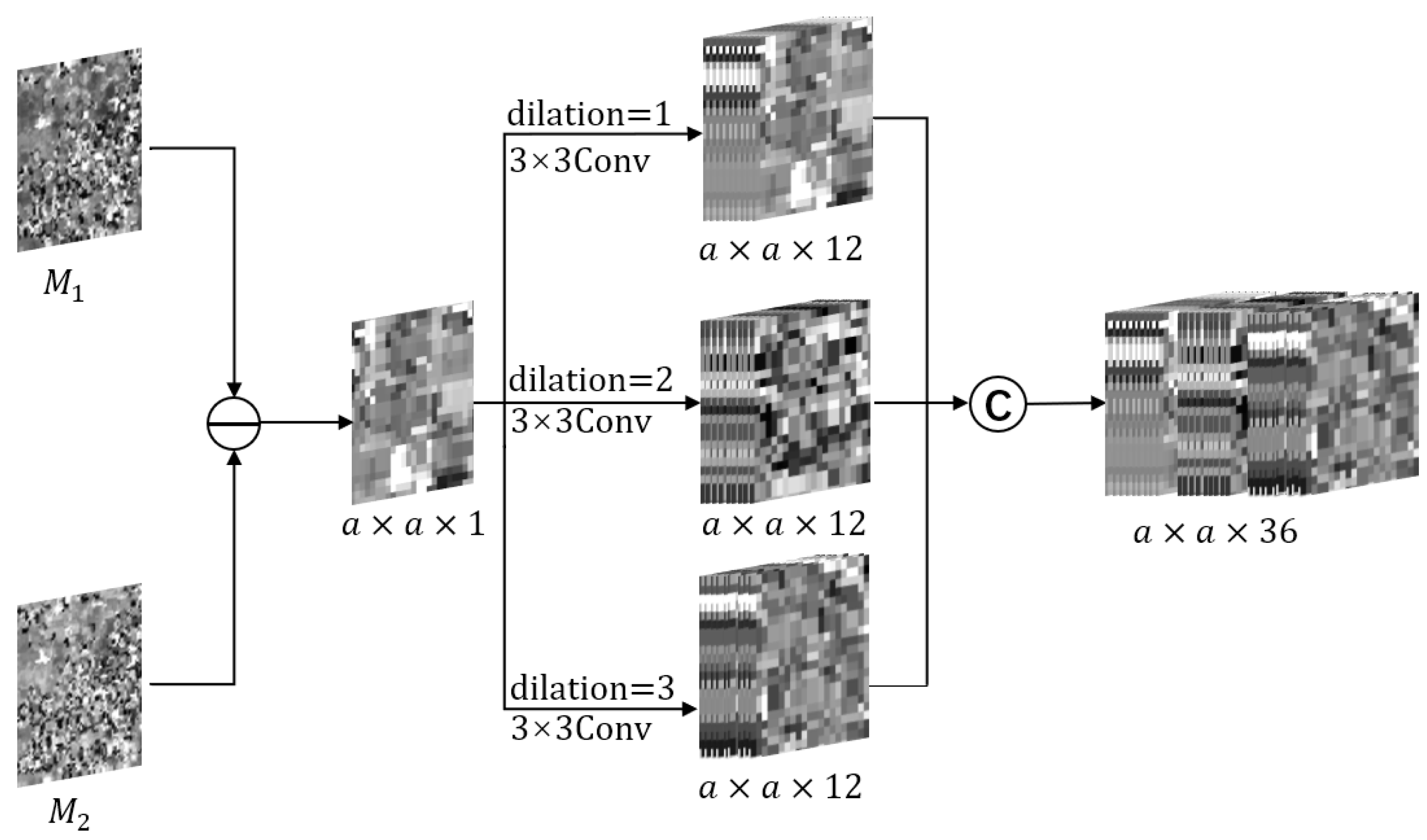
- A multiscale mechanism is used to extract temporal and spatial change information from low-spatial resolution images at multiple scales, which is to provide more detailed information for the subsequent fusion process.
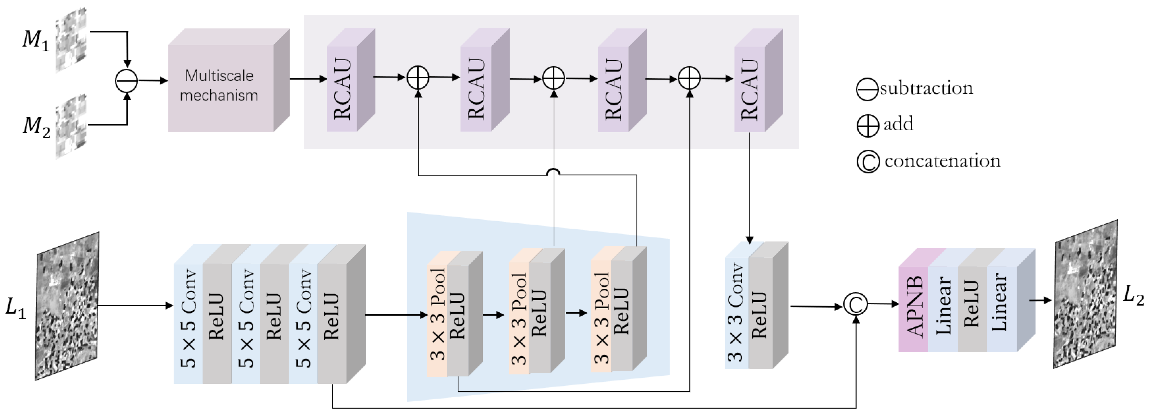
- A residual channel attention upsampling (RCAU) module is designed to upsample the low-spatial resolution image. Inspired by DenseNet [34] and FPN [35] structures, the rich spatial details of high-spatial resolution images are used to complement the spatial loss of low-spatial resolution images during the upsampling process. This collaborative network structure makes the spatial and spectral information of the reconstructed images more accurate.
- A non-local attention mechanism is proposed to reconstruct the fused image by learning the global contextual information, which can improve the accuracy of the temporal and spatial information of the fused image.
3. Materials and Methods
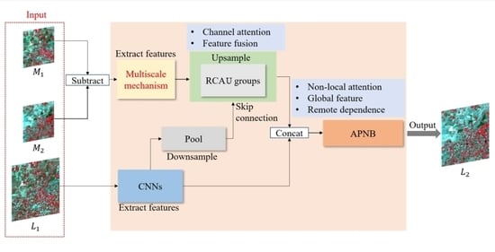
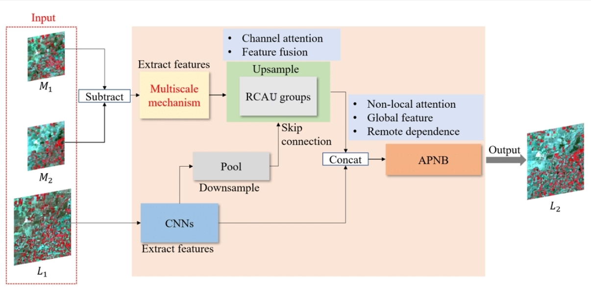
3.1. MANet Architecture
- A sub-network is used to process residual low-spatial resolution images, extracting the temporal and spatial variation information.
- A sub-network is used to process high-spatial resolution images, extracting spatial and spectral information.
- To obtain more accurate fused images, a new fusion strategy is introduced to further learn the global temporal and spatial change information of the fused image.
3.2. Multiscale Mechanism
3.3. Attentional Mechanism
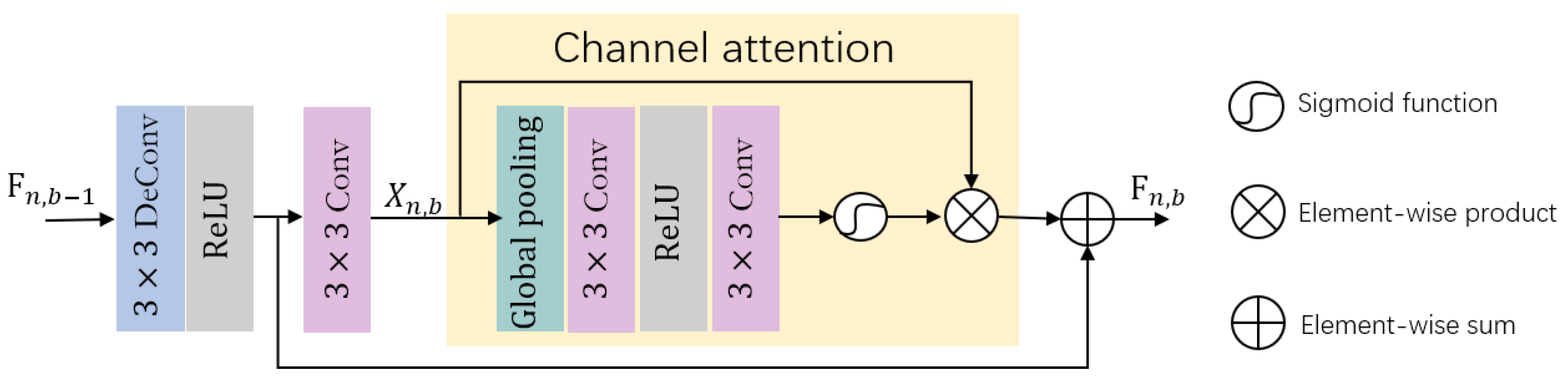
3.3.1. RCAU Module
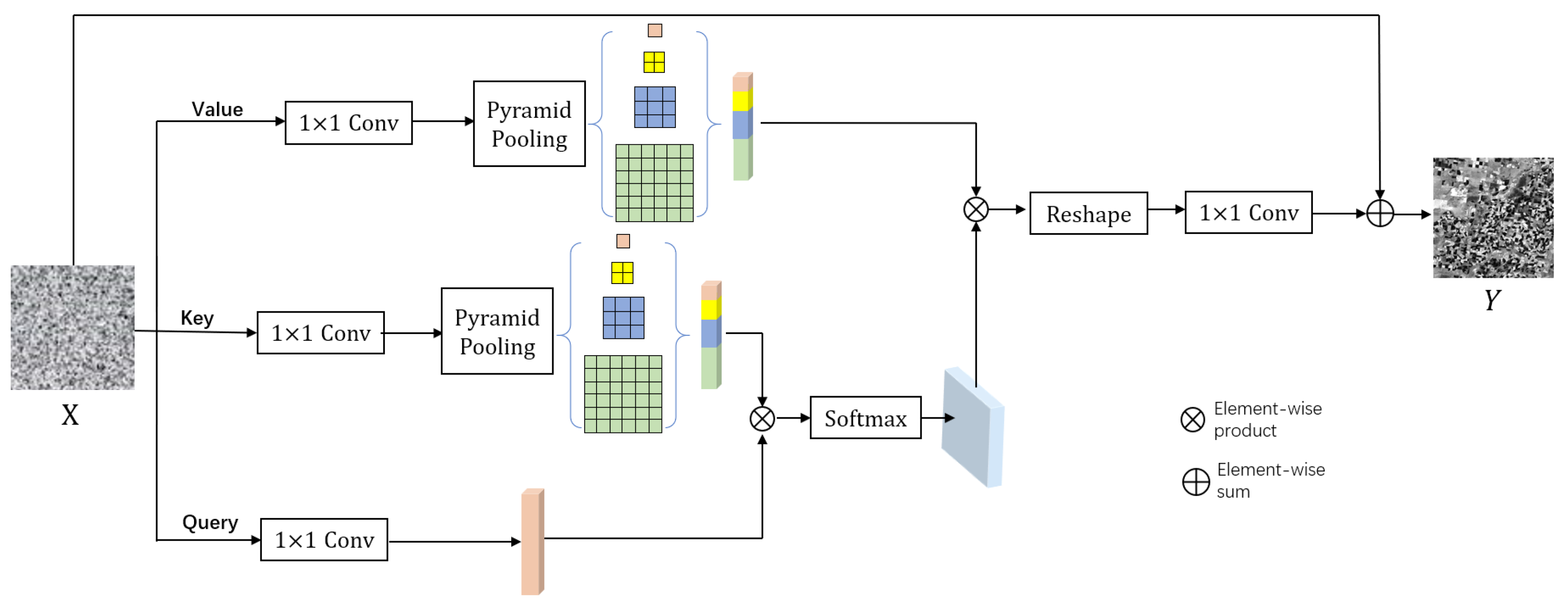
3.3.2. APNB Architecture
3.4. Loss Function
4. Experiments
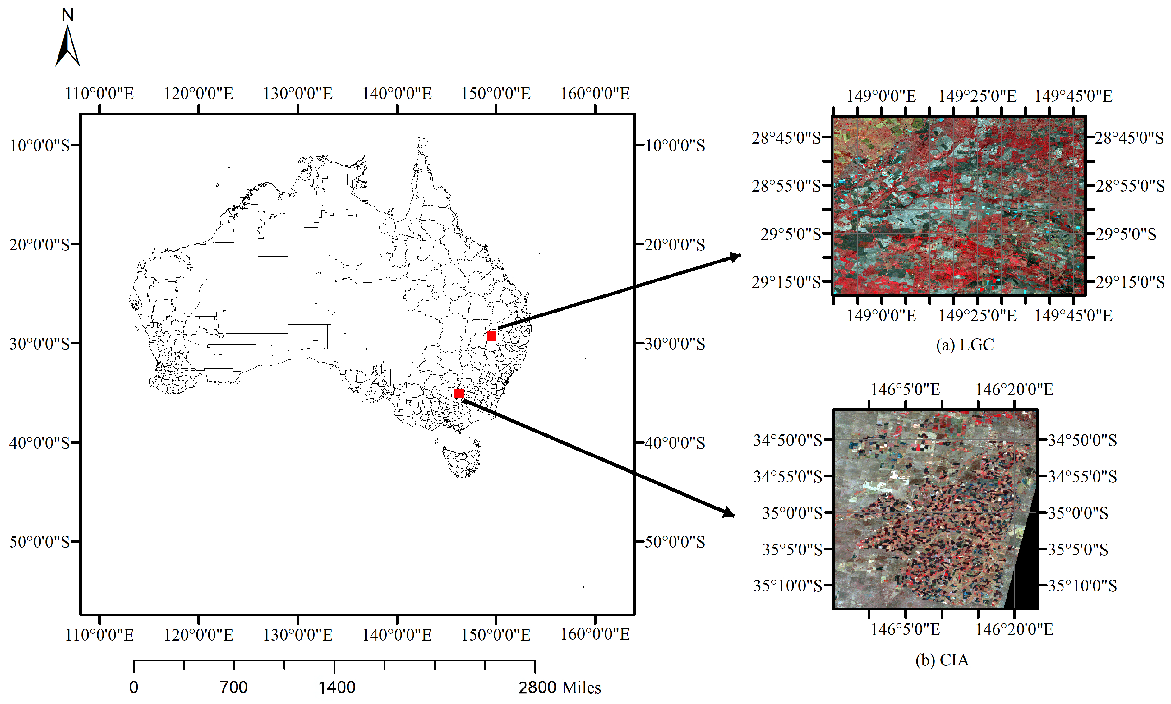
4.1. Datasets
4.2. Evaluation Indicators
4.3. Parameter Setting
4.4. Experiment Results
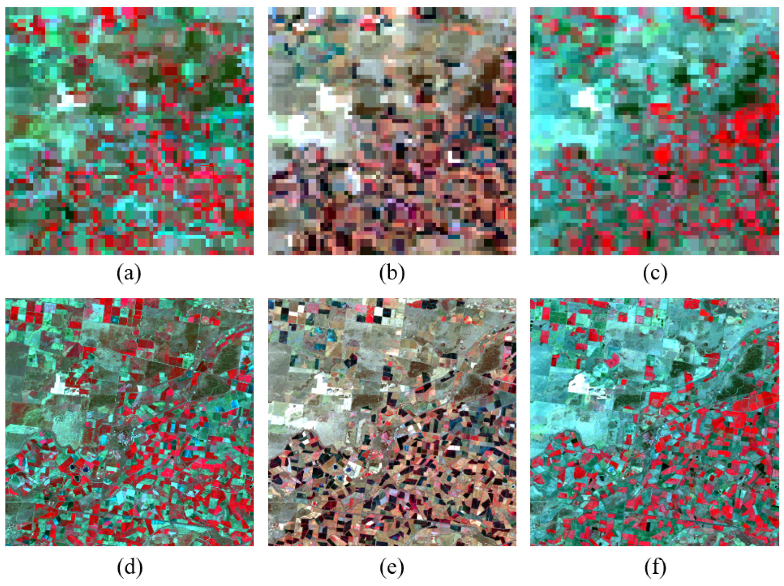
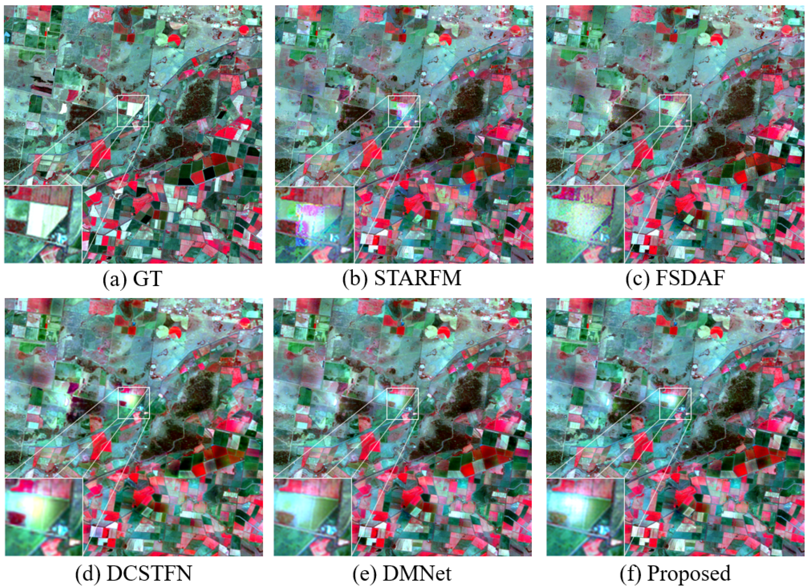
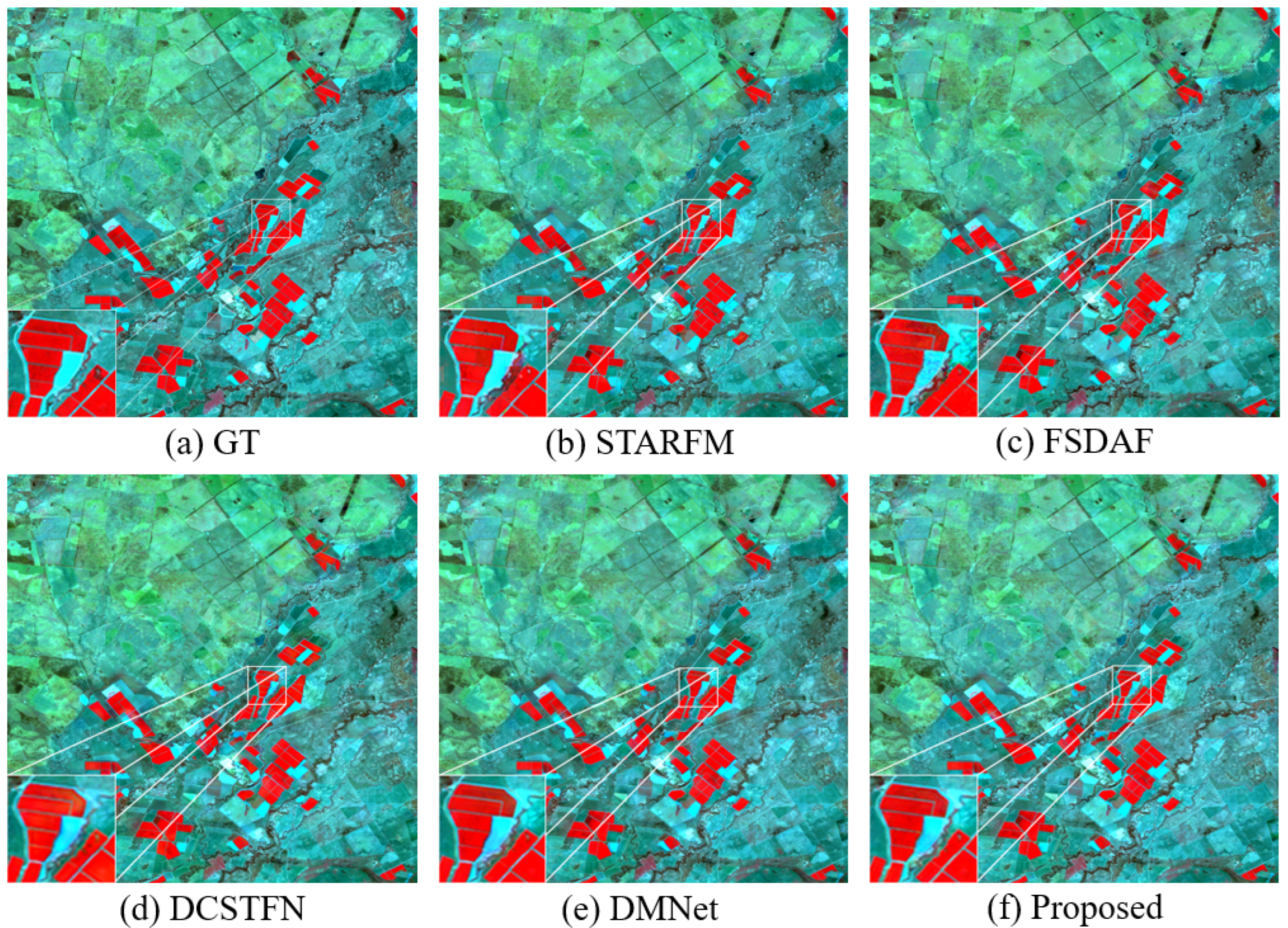
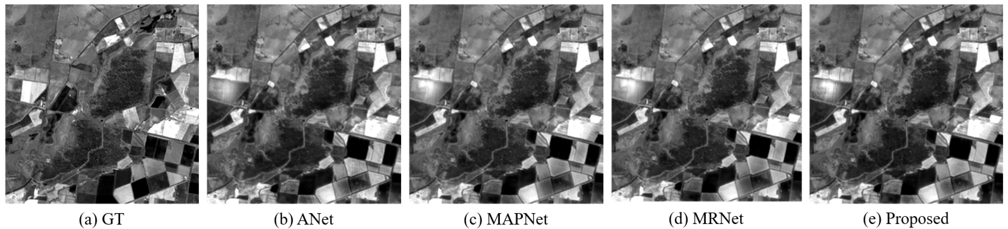
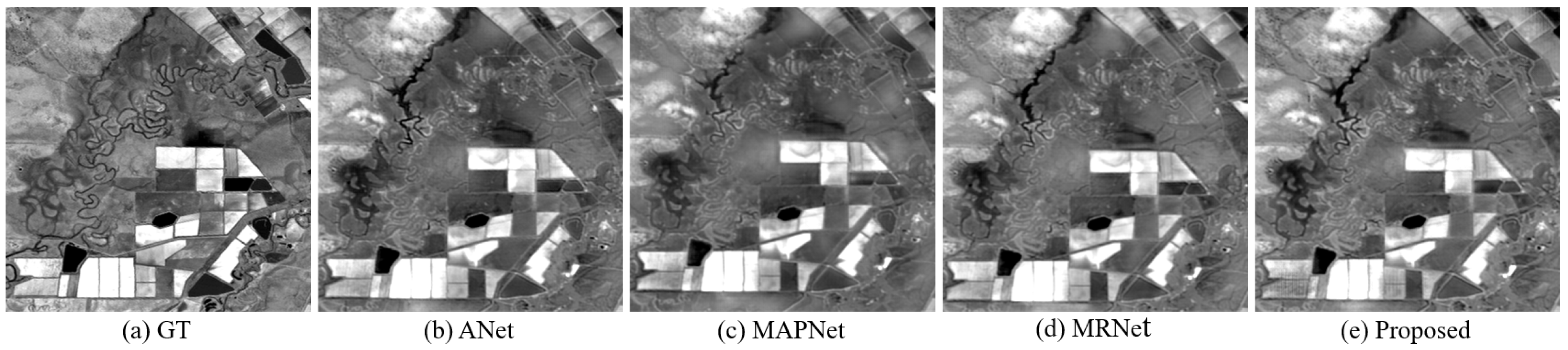
4.4.1. Subjective Evaluation
4.4.2. Objective Evaluation
5. Discussion
5.1. Ablation Experiments
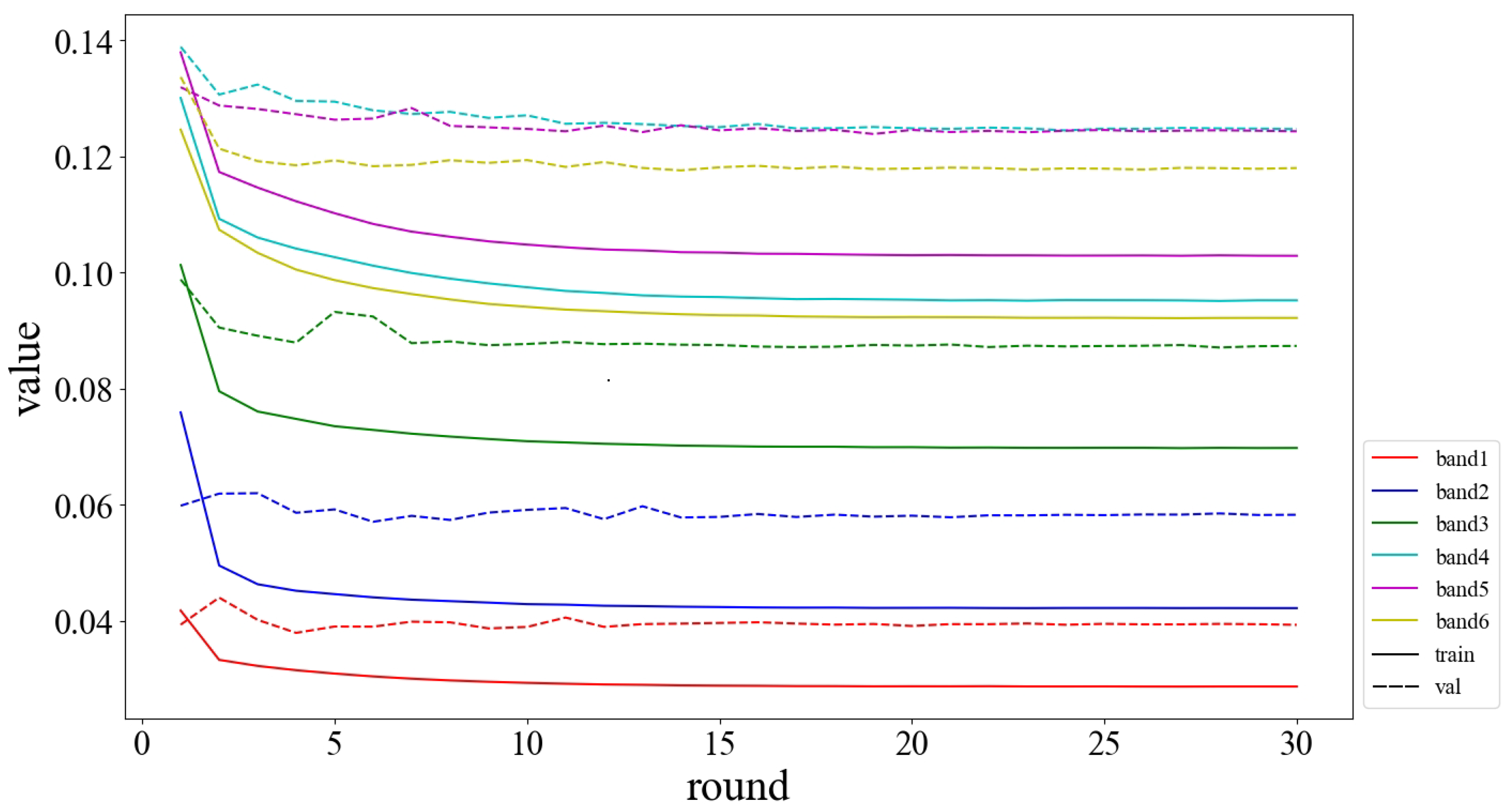
5.2. Loss Curves and the Number of Training Parameters
6. Conclusions
- The multiscale mechanism is used to extract the temporal and spatial variation of a low-spatial resolution image. The final experimental results indicated that the extraction of detail features at different scales can make the network retain more useful temporal and spatial details, and the prediction result is closer to the real result.
- By designing the RCAU module, we not only realize the upsampling of feature maps with low-spatial resolution, but also reduce the loss of detail information by the weighting operation, which is more conducive to the reconstruction of low-spatial resolution image pixels.
- In the fusion process, we have designed a new fusion strategy. The APNB module was added after the initial fusion image, which can effectively extract global spatial and temporal information. Experimental results show that our method can better capture the spatial details and spectral information of the predicted image.
Author Contributions
Funding
Data Availability Statement
Acknowledgments
Conflicts of Interest
References
- Saah, D.; Tenneson, K.; Matin, M.; Uddin, K.; Cutter, P.; Poortinga, A.; Nguyen, Q.H.; Patterson, M.; Johnson, G.; Markert, K.; et al. Land Cover Mapping in Data Scarce Environments: Challenges and Opportunities. Front. Environ. Sci. 2019, 7, 150. [Google Scholar] [CrossRef]
- Li, M.; Sun, D.; Goldberg, M.; Stefanidis, A. Derivation of 30-m-resolution water maps from TERRA/MODIS and SRTM. Remote Sens. Environ. 2013, 134, 417–430. [Google Scholar] [CrossRef]
- Lv, Z.; Liu, T.F.; Zhang, P.; Benediktsson, J.A.; Lei, T.; Zhang, X. Novel adaptive histogram trend similarity approach for land cover change detection by using bitemporal very-high-resolution remote sensing images. IEEE Trans. Geosci. Remote Sens. 2019, 57, 9554–9574. [Google Scholar] [CrossRef]
- Ma, Y.; Chen, F.; Liu, J.; He, Y.; Duan, J.; Li, X. An Automatic Procedure for Early Disaster Change Mapping Based on Optical remote sensing. Remote Sens. 2016, 8, 272. [Google Scholar] [CrossRef]
- Huang, B.; Wang, J.; Song, H.; Fu, D.; Wong, K. Generating High Spatiotemporal Resolution Land Surface Temperature for Urban Heat Island Monitoring. IEEE Geosci. Remote Sens. Lett. 2013, 10, 1011–1015. [Google Scholar] [CrossRef]
- Dai, P.; Zhang, H.; Zhang, L.; Shen, H. A remote sensing Spatiotemporal Fusion Model of Landsat and Modis Data via Deep Learning. In Proceedings of the IGARSS 2018—2018 IEEE International Geoscience and Remote Sensing Symposium, Valencia, Spain, 22–27 July 2018; pp. 7030–7033. [Google Scholar]
- Song, H.; Huang, B. Spatiotemporal satellite image fusion through one-pair image learning. IEEE Trans. Geosci. Remote Sens. 2013, 51, 1883–1896. [Google Scholar] [CrossRef]
- Li, W.; Cao, D.; Peng, Y.; Yang, C. MSNet: A Multi-Stream Fusion Network for remote sensing Spatiotemporal Fusion Based on Transformer and Convolution. Remote Sens. 2021, 13, 3724. [Google Scholar] [CrossRef]
- Wu, M.; Wang, C. Spatial and Temporal Fusion of remote sensing Data using wavelet transform. In Proceedings of the 2011 International Conference on Remote Sensing, Environment and Transportation Engineering, Nanjing, China, 24–26 June 2011; pp. 1581–1584. [Google Scholar]
- Gu, X.; Han, L.; Wang, J.; Huang, W.; He, X. Estimation of maize planting area based on wavelet fusion of multi-resolution images. Trans. Chin. Soc. Agric. Eng. 2012, 28, 203–209. [Google Scholar] [CrossRef]
- Acerbi-Junior, F.W.; Clevers, J.G.P.W.; Schaepman, M.E. The assessment of multi-sensor image fusion using wavelet transforms for mapping the Brazilian Savanna. Int. J. Appl. Earth Obs. Geoinform. 2006, 8, 278–288. [Google Scholar] [CrossRef]
- Shevyrnogov, A.; Trefois, P.; Vysotskaya, G. Multi-satellite data merge to combine NOAA AVHRR efficiency with Landsat-6 MSS spatial resolution to study vegetation dynamics. Adv. Space Res. 2000, 26, 1131–1133. [Google Scholar] [CrossRef]
- Gao, F.; Masek, J.; Schwaller, M.; Hall, F. On the blending of the Landsat and MODIS surface reflectance: Predicting daily Landsat surface reflectance. IEEE Trans. Geosci. Remote Sens. 2006, 44, 2207–2218. [Google Scholar] [CrossRef]
- Zhu, X.; Chen, J.; Gao, F.; Chen, X.; Masek, J.G. An enhanced spatial and temporal adaptive reflectance fusion model for complex heterogeneous regions. Remote Sens. Environ. 2010, 114, 2610–2623. [Google Scholar] [CrossRef]
- Hilker, T.; Wulder, M.A.; Coops, N.C.; Linke, J.; McDermid, G.; Masek, J.G.; Gao, F.; White, J.C. A new data fusion model for high-spatial-and temporal-resolution mapping of forest disturbance based on Landsat and MODIS. Remote Sens. Environ. 2009, 113, 1613–1627. [Google Scholar] [CrossRef]
- Crist, E.P.; Kauth, R.J. The tasseled cap de-mystified. Photogramm. Eng. Remote Sens. 1986, 52, 81–86. [Google Scholar]
- Healey, S.P.; Cohen, W.B.; Yang, Z.; Krankina, O.N. Comparison of Tasseled Cap-based Landsat data structures for use in forest disturbance detection. Remote Sens. Environ. 2005, 97, 301–310. [Google Scholar] [CrossRef]
- Li, W.; Zhang, X.; Peng, Y.; Dong, M. DMNet: A Network Architecture Using Dilated Convolution and Multiscale Mechanisms for Spatiotemporal Fusion of remote sensing Images. IEEE Sens. J. 2020, 20, 12190–12202. [Google Scholar] [CrossRef]
- Zhukov, B.; Oertel, D.; Lanzl, F.; Reinhackel, G. Unmixing-based multisensor multiresolution image fusion. IEEE Trans. Geosci. Remote Sens. 1999, 37, 1212–1226. [Google Scholar] [CrossRef]
- Wu, M.; Niu, Z.; Wang, C.; Wu, C.; Wang, L. Use of MODIS and Landsat time series data to generate high-resolution temporal synthetic Landsat data using a spatial and temporal reflectance fusion model. J. Appl. Remote Sens. 2012, 6, 063507. [Google Scholar] [CrossRef]
- Zhu, X.; Helmer, E.H.; Gao, F.; Liu, D.; Chen, J.; Lefsky, M.A. A flexible spatiotemporal method for fusing satellite images with different resolutions. Remote Sens. Environ. 2016, 172, 165–177. [Google Scholar] [CrossRef]
- Huang, B.; Song, H. Spatiotemporal reflectance fusion via sparse representation. IEEE Trans. Geosci. Remote Sens. 2012, 50, 3707–3716. [Google Scholar] [CrossRef]
- Wei, J.; Wang, L.; Liu, P.; Song, W. Spatiotemporal Fusion of remote sensing Images with Structural Sparsity and Semi-Coupled Dictionary Learning. Remote Sens. 2017, 9, 21. [Google Scholar] [CrossRef] [Green Version]
- Wu, B.; Huang, B.; Zhang, L. An error-bound-regularized sparse coding for spatiotemporal reflectance fusion. IEEE Trans. Geosci. Remote Sens. 2015, 53, 6791–6803. [Google Scholar] [CrossRef]
- Peng, Y.; Li, W.; Luo, X.; Du, J.; Zhang, X.; Gan, Y.; Gao, X. Spatiotemporal Reflectance Fusion via Tensor Sparse Representation. IEEE Trans. Geosci. Remote Sens. 2021, 60, 1–18. [Google Scholar] [CrossRef]
- Dong, C.; Loy, C.; He, K.; Tang, X. Image Super-Resolution Using Deep Convolutional Networks. IEEE Trans. Pattern Anal. Mach. Intell. 2015, 38, 295–307. [Google Scholar] [CrossRef]
- Tan, Z.; Yue, P.; Di, L.; Tang, J. Deriving High Spatiotemporal remote sensing Images Using Deep Convolutional Network. Remote Sens. 2018, 10, 1066. [Google Scholar] [CrossRef]
- Tan, Z.; Di, L.; Zhang, M.; Guo, L.; Gao, M. An enhanced deep convolutional model for spatiotemporal image fusion. Remote Sens. 2019, 11, 2898. [Google Scholar] [CrossRef]
- Song, H.; Liu, Q.; Wang, G.; Hang, R.; Huang, B. Spatiotemporal satellite image fusion using deep convolutional neural networks. IEEE J. Sel. Top. Appl. Earth Obs. Remote Sens. 2018, 11, 821–829. [Google Scholar] [CrossRef]
- Liu, X.; Deng, C.; Chanussot, J.; Hong, D.; Zhao, B. StfNet: A two-stream convolutional neural network for spatiotemporal image fusion. IEEE Trans. Geosci. Remote Sens. 2019, 57, 6552–6564. [Google Scholar] [CrossRef]
- Tan, Z.; Gao, M.; Li, X.; Jiang, L. A Flexible Reference-Insensitive Spatiotemporal Fusion Model for remote sensing Images Using Conditional Generative Adversarial Network. IEEE Trans. Geosci. Remote Sens. 2021, 60, 1–13. [Google Scholar] [CrossRef]
- Li, W.; Yang, C.; Peng, Y.; Zhang, X. A Multi-Cooperative Deep Convolutional Neural Network for Spatiotemporal Satellite Image Fusion. IEEE J. Sel. Top. Appl. Earth Obs. Remote Sens. 2021, 14, 10174–10188. [Google Scholar] [CrossRef]
- Yang, G.; Liu, H.; Zhong, X.; Chen, L.; Qian, Y. Temporal and Spatial Fusion of Remote Sensing Images: A Review. Comput. Eng. Appl. 2022, 58, 27–40. [Google Scholar] [CrossRef]
- Huang, G.; Liu, Z.; Maaten, L.V.; Weinberger, K.Q. Densely Connected Convolutional Networks. In Proceedings of the 2017 IEEE Conference on Computer Vision and Pattern Recognition (CVPR), Honolulu, HI, USA, 21–26 July 2017; pp. 2261–2269. [Google Scholar]
- Lin, T.; Dollár, P.; Girshick, R.; He, K.; Hariharan, B.; Belongie, S. Feature Pyramid Networks for Object Detection. In Proceedings of the 2017 IEEE Conference on Computer Vision and Pattern Recognition (CVPR), Honolulu, HI, USA, 21–26 July 2017; pp. 936–944. [Google Scholar]
- Zhu, Z.; Xu, M.; Bai, S.; Huang, T.; Bai, X. Asymmetric Non-Local Neural Networks for Semantic Segmentation. In Proceedings of the 2019 IEEE/CVF International Conference on Computer Vision (ICCV), Seoul, Korea, 27 October–2 November 2019; pp. 593–602. [Google Scholar]
- Yu, F.; Koltun, V. Multi-Scale Context Aggregation by Dilated Convolutions. In Proceedings of the 4th International Conference on Learning Representations, ICLR, San Juan, Puerto Rico, 2–4 May 2016. [Google Scholar]
- Zhang, Y.; Li, K.; Li, K.; Wang, L.; Zhong, B.; Fu, Y. Image Super-Resolution Using Very Deep Residual Channel Attention Networks. In Proceedings of the European Conference on Computer Vision, Munich, Germany, 8–14 September 2018; pp. 294–310. [Google Scholar]
- Hu, J.; Shen, L.; Albanie, S.; Sun, G.; Wu, E. Squeeze-and-excitation networks. IEEE Trans. Pattern Anal. Mach. Intell. 2020, 42, 2011–2023. [Google Scholar] [CrossRef] [PubMed]
- Fu, J.; Liu, J.; Tian, H.; Li, Y.; Bao, Y.; Fang, Z.; Lu, H. Dual Attention Network for Scene Segmentation. In Proceedings of the 2019 IEEE/CVF Conference on Computer Vision and Pattern Recognition (CVPR), Long Beach, CA, USA, 15–20 June 2019; pp. 3146–3154. [Google Scholar]
- Wang, X.; Girshick, R.; Gupta, A.; He, K. Non-local neural networks. In Proceedings of the IEEE Conference on Computer Vision and Pattern Recognition, Los Alamitos, CA, USA, 18–23 June 2018; pp. 7794–7803. [Google Scholar]
- Wang, S.; Hou, X.; Zhao, X. Automatic Building Extraction From High-Resolution Aerial Imagery via Fully Convolutional Encoder-Decoder Network with Non-Local Block. IEEE Access 2020, 8, 7313–7322. [Google Scholar] [CrossRef]
- Lai, W.S.; Huang, J.B.; Ahuja, N.; Yang, M.H. Fast and Accurate Image Super-Resolution with Deep Laplacian Pyramid Networks. IEEE Trans. Pattern Anal. Mach. Intell. 2019, 41, 2599–2613. [Google Scholar] [CrossRef]
- Tan, Z.; Gao, M.; Yuan, J.; Jiang, L.; Duan, H. A Robust Model for MODIS and Landsat Image Fusion Considering Input Noise. IEEE Trans. Geosci. Remote Sens. 2022, 60, 5407217. [Google Scholar] [CrossRef]
- Zhao, H.; Gallo, O.; Frosio, I.; Kautz, J. Loss Functions for Image Restoration with Neural Networks. IEEE Trans. Comput. Imaging 2017, 3, 47–57. [Google Scholar] [CrossRef]
- Emelyanova, I.V.; McVicar, T.R.; Van Niel, T.G.; Li, L.T.; Van Dijk, A.I. Assessing the accuracy of blending Landsat–MODIS surface reflectances in two landscapes with contrasting spatial and temporal dynamics: A framework for algorithm selection. Remote Sens. Environ. 2013, 133, 193–209. [Google Scholar] [CrossRef]
- Li, F.; Jupp, D.L.B.; Reddy, S.; Lymburner, L.; Mueller, N.; Tan, P.; Islam, A. An Evaluation of the Use of Atmospheric and BRDF Correction to Standardize Landsat Data. IEEE J. Sel. Top. Appl. Earth Obs. Remote Sens. 2010, 3, 257–270. [Google Scholar] [CrossRef]
- Berk, A.; Anderson, G.P.; Bernstein, L.S.; Acharya, P.K.; Dothe, H.; Matthew, M.; Adler-Golden, S.; Chetwynd, J.; Richtsmeier, S.; Pukall, B.; et al. MODTRAN4 radiative transfer modeling for atmospheric correction. In Proceedings of the SPIE, Optical Spectroscopic Techniques and Instrumentation for Atmospheric and Space Research III, Denver, CO, USA, 20 October 1999. [Google Scholar]
- Van Niel, T.G.; McVicar, T.R. Determining temporal windows for crop discrimination with remote sensing: A case study in south-eastern Australia. Comput. Electron. Agric. 2004, 45, 91–108. [Google Scholar] [CrossRef]
- Wang, Z.; Bovik, A.C.; Sheikh, H.R.; Simoncelli, E.P. Image quality assessment: From error visibility to structural similarity. IEEE Trans. Image Process. 2004, 13, 600–612. [Google Scholar] [CrossRef]
- Ponomarenko, N.; Ieremeiev, O.; Lukin, V.; Egiazarian, K.; Carli, M. Modified image visual quality metrics for contrast change and mean shift accounting. In Proceedings of the 2011 11th International Conference the Experience of Designing and Application of CAD Systems in Microelectronics (CADSM), Polyana, Ukraine, 23–25 February 2011; pp. 305–311. [Google Scholar]
- Alparone, L.; Wald, L.; Chanussot, J.; Thomas, C.; Gamba, P.; Bruce, L. Comparison of Pansharpening Algorithms: Outcome of the 2006 GRS-S Data-Fusion Contest. IEEE Trans. Geosci. Remote Sens. 2007, 45, 3012–3021. [Google Scholar] [CrossRef] [Green Version]


| Evaluation | Band | Method | ||||
|---|---|---|---|---|---|---|
| STARFM | FSDAF | DCSTFN | DMNet | Proposed | ||
| SSIM | Band1 | 0.8731 | 0.9037 | 0.9355 | 0.9368 | 0.9455 |
| Band2 | 0.8527 | 0.9172 | 0.9304 | 0.9304 | 0.9351 | |
| Band3 | 0.7938 | 0.8578 | 0.8915 | 0.8905 | 0.8989 | |
| Band4 | 0.7329 | 0.8210 | 0.8231 | 0.8271 | 0.8319 | |
| Band5 | 0.7197 | 0.8109 | 0.8165 | 0.8187 | 0.8274 | |
| Band6 | 0.7260 | 0.8194 | 0.8383 | 0.8379 | 0.8432 | |
| Average | 0.7830 | 0.8550 | 0.8726 | 0.8736 | 0.8803 | |
| PSNR | Band1 | 27.4332 | 37.2104 | 38.3779 | 38.3696 | 39.2152 |
| Band2 | 24.3359 | 36.0368 | 36.4337 | 36.3136 | 36.8910 | |
| Band3 | 24.5396 | 31.3339 | 33.2257 | 32.8116 | 33.2862 | |
| Band4 | 19.6533 | 26.9470 | 28.7492 | 28.5944 | 28.8370 | |
| Band5 | 20.8408 | 28.0493 | 28.4029 | 28.1894 | 28.5474 | |
| Band6 | 22.1580 | 25.0635 | 29.8863 | 29.7228 | 29.9921 | |
| Average | 23.1601 | 30.7735 | 32.5126 | 32.3336 | 32.7948 | |
| CC | Band1 | 0.3898 | 0.8014 | 0.8374 | 0.8382 | 0.8547 |
| Badn2 | 0.3965 | 0.7988 | 0.8603 | 0.8581 | 0.8658 | |
| Band3 | 0.5883 | 0.8302 | 0.8912 | 0.8854 | 0.8882 | |
| Band4 | 0.5039 | 0.8161 | 0.8265 | 0.8195 | 0.8272 | |
| Band5 | 0.6855 | 0.8977 | 0.9015 | 0.8989 | 0.9060 | |
| Band6 | 0.6927 | 0.9060 | 0.9153 | 0.9126 | 0.9162 | |
| Average | 0.5428 | 0.8417 | 0.8720 | 0.8688 | 0.8764 | |
| RMSE | Band1 | 0.0124 | 0.0124 | 0.0123 | 0.0122 | 0.0112 |
| Band2 | 0.0156 | 0.0162 | 0.0156 | 0.0158 | 0.0149 | |
| Band3 | 0.0227 | 0.0234 | 0.0226 | 0.0239 | 0.0229 | |
| Band4 | 0.0387 | 0.0408 | 0.0387 | 0.0395 | 0.0385 | |
| Band5 | 0.0386 | 0.0399 | 0.0386 | 0.0394 | 0.0382 | |
| Band6 | 0.0330 | 0.0329 | 0.0324 | 0.0330 | 0.0324 | |
| Average | 0.0268 | 0.0276 | 0.0267 | 0.0273 | 0.0264 | |
| Evaluation | Band | Method | ||||
|---|---|---|---|---|---|---|
| STARFM | FSDAF | DCSTFN | DMNet | Proposed | ||
| SSIM | Band1 | 0.8846 | 0.9264 | 0.9361 | 0.9368 | 0.9384 |
| Band2 | 0.8837 | 0.9300 | 0.9489 | 0.9304 | 0.9488 | |
| Band3 | 0.8401 | 0.9241 | 0.9262 | 0.8905 | 0.9303 | |
| Band4 | 0.8071 | 0.8803 | 0.8901 | 0.8971 | 0.8975 | |
| Band5 | 0.7860 | 0.8693 | 0.8706 | 0.8687 | 0.8842 | |
| Band6 | 0.7908 | 0.8615 | 0.8714 | 0.8779 | 0.8804 | |
| Average | 0.8321 | 0.8986 | 0.9072 | 0.9002 | 0.9133 | |
| PSNR | Band1 | 30.4687 | 38.5891 | 39.0567 | 39.5980 | 39.6168 |
| Band2 | 23.3251 | 37.1057 | 38.0523 | 38.1447 | 38.2195 | |
| Band3 | 23.6144 | 35.0483 | 35.9674 | 35.7742 | 36.0948 | |
| Band4 | 17.4570 | 31.2650 | 31.5236 | 31.4327 | 31.8561 | |
| Band5 | 20.3062 | 30.2034 | 30.9916 | 30.8822 | 31.2151 | |
| Band6 | 21.9842 | 31.0435 | 32.1594 | 31.9054 | 32.2980 | |
| Average | 22.8593 | 33.8758 | 34.6252 | 34.6229 | 34.8834 | |
| CC | Band1 | 0.7697 | 0.8802 | 0.8973 | 0.9012 | 0.9090 |
| Band2 | 0.8775 | 0.8901 | 0.8943 | 0.8939 | 0.9003 | |
| Band3 | 0.8272 | 0.8969 | 0.9052 | 0.9067 | 0.9079 | |
| Band4 | 0.8993 | 0.9090 | 0.9198 | 0.9183 | 0.9209 | |
| Band5 | 0.7816 | 0.9216 | 0.9263 | 0.9242 | 0.9298 | |
| Band6 | 0.7270 | 0.9203 | 0.9228 | 0.9252 | 0.9264 | |
| Average | 0.8137 | 0.9030 | 0.9110 | 0.9116 | 0.9157 | |
| RMSE | Band1 | 0.0122 | 0.0139 | 0.0122 | 0.0119 | 0.0117 |
| Band2 | 0.0134 | 0.0132 | 0.0130 | 0.0130 | 0.0131 | |
| Band3 | 0.0164 | 0.0167 | 0.0162 | 0.0166 | 0.0163 | |
| Band4 | 0.0268 | 0.0276 | 0.0268 | 0.0271 | 0.0259 | |
| Band5 | 0.0291 | 0.0297 | 0.0291 | 0.0298 | 0.0286 | |
| Band6 | 0.0277 | 0.0271 | 0.0257 | 0.0266 | 0.0254 | |
| Average | 0.0209 | 0.0214 | 0.0205 | 0.0208 | 0.0202 | |
| Dataset | Index | ANet | MAPNet | MRNet | MANet |
|---|---|---|---|---|---|
| CIA | SSIM | 0.8794 | 0.8791 | 0.8788 | 0.8803 |
| RMSE | 0.0266 | 0.0267 | 0.0267 | 0.0264 | |
| LGC | SSIM | 0.9132 | 0.9131 | 0.9133 | 0.9133 |
| RMSE | 0.0203 | 0.0204 | 0.0203 | 0.0202 |
| Method | STARFM | FSDAF | DCSTFN | DMNet | MANet |
|---|---|---|---|---|---|
| Training parameters | - | - | 298,177 | 327,061 | 77,171 |
Publisher’s Note: MDPI stays neutral with regard to jurisdictional claims in published maps and institutional affiliations. |
© 2022 by the authors. Licensee MDPI, Basel, Switzerland. This article is an open access article distributed under the terms and conditions of the Creative Commons Attribution (CC BY) license (https://creativecommons.org/licenses/by/4.0/).
Share and Cite
Cao, H.; Luo, X.; Peng, Y.; Xie, T. MANet: A Network Architecture for Remote Sensing Spatiotemporal Fusion Based on Multiscale and Attention Mechanisms. Remote Sens. 2022, 14, 4600. https://doi.org/10.3390/rs14184600
Cao H, Luo X, Peng Y, Xie T. MANet: A Network Architecture for Remote Sensing Spatiotemporal Fusion Based on Multiscale and Attention Mechanisms. Remote Sensing. 2022; 14(18):4600. https://doi.org/10.3390/rs14184600
Chicago/Turabian StyleCao, Huimin, Xiaobo Luo, Yidong Peng, and Tianshou Xie. 2022. "MANet: A Network Architecture for Remote Sensing Spatiotemporal Fusion Based on Multiscale and Attention Mechanisms" Remote Sensing 14, no. 18: 4600. https://doi.org/10.3390/rs14184600