1. Introduction
With the rapid development of earth observation technology, there are more and more remote sensing sensors providing numerous images of the earth surface. The demand for rapid analysis of vast quantities of remote sensing images has increased significantly. Classification of these massive images is one of the most important tasks. Compared with pixel-level and object-level classification, image scene classification takes the scenes, i.e., the image blocks, as the classification units and labels them with semantic descriptors [
1,
2]. It is a promising way for classifying the current high-resolution remote sensing images, and plays an important role in natural disaster monitoring [
3] and functional area classification [
4].
Similar to image classification in the computer vision domain, the key to remote sensing image scene classification is the extraction of image scene features. Due to the powerful feature extraction ability and successful application in various domains, deep learning has been widely applied to remote sensing image scene classification in recent years. However, these deep-learning-based scene classification methods [
5,
6,
7] usually require a large number of labeled samples. Because it is difficult to obtain enough labeled samples for all classes, it is of great significance for methods which can recognize the image scenes that are not seen in the training stage. In this case, zero-shot learning (ZSL) methods which does’t require any labeled samples have recently attracted much attention [
8].
Derived from transfer learning [
9], zero-shot learning is the training of a model using a large number of labeled samples called the seen classes of samples, and then using the model to predict the labels of unseen classes of samples, where the samples of seen and unseen classes are not identical. Taking the semantic features of the seen and unseen classes as the auxiliary information, zero-shot learning leverages the knowledge learned from the seen classes and applies them to the unseen classes. By now, many methods have emerged for zero-shot learning in the computer vision domain. The common strategy for ZSL is to build a mapping between the visual features of the seen images and the semantic features of the seen classes, and then apply the mapping to the unseen images [
10,
11]. This kind of methods often suffer from the hubness problem [
12] or the domain shift problem [
13]. Recently, more and more works are using the generative methods to tackle ZSL problem. Some works propose to utilize generative methods to generate a certain number of visual features for each unseen class conditioned on their semantic features [
14]. The classes of the unseen images can be predicted by applying nearest-neighbor search algorithms. In the meantime, some works propose to apply the generative method to embed both the image visual features and the class semantic features into the latent space, and then match or align these latent features [
15].
Due to the specific characteristics of remote sensing images, more challenges for zero-shot learning exist in remote sensing. For example, unlike the labels of the natural images, labels of remote sensing images can’t actually reflect the semantic information of the classes. Moreover, there often exist scale variation and arbitrary orientation of geo-spatial elements in remote sensing images [
16]. The images also show large intraclass differences and large interclass similarities [
17,
18]. With these challenges, many methods [
16,
19] have been proposed to address the zero-shot classification problem of remote sensing image scenes based on existing zero-shot learning works. For example, with the aim to achieve the cross-modal feature matching and address the intraclass differences and interclass similarities, a set of loss constraints has been designed in [
16]; and to obtain the high-quality semantic representation of remote sensing image scenes, a remote sensing knowledge graph has been constructed [
19]. In recent works, researchers have also started to use generative methods to tackle zero-shot remote sensing image scene classification. In the work of Li et al. [
19], two variational autoencoders (VAE) have been utilized to project the visual features of image scenes and the semantic features of the classes into the latent space, after which the reconstruction loss and the distribution matching loss are used to achieve cross-modal feature alignment.
However, for the generative model of VAEs used for zero-shot image scene classification, an important component is the metric measuring the reconstruction quality. It calculates the element-wise square error between the true visual/semantic features and the generated visual/semantic features, to produce the reconstruction loss. This way of generating reconstruction loss may be not suitable for measuring the reconstruction quality. For example, when making some kind of transformation to the images, people may not notice the transformation; however, a large square error is produced. In light of that, this paper proposes to integrate the generative adversarial network (GAN), another kind of generative model, with the VAE models towards a cross-modal feature alignment for zero-shot remote sensing image scene classification. Our concept is augmentation of the dual VAEs with the GAN discriminator, and adopt it to learn a suitable reconstruction quality metric for VAE [
20]. For two different VAE models of the dual VAEs used for two different modalities, i.e., the visual and the semantic modalities, we propose to equip each VAE with a discriminator while using one cross-modal discriminator for both VAEs. Moreover, considering the characteristics of intraclass differences and interclass similarities among the remote sensing images, we have also designed the matching loss between the cross-modal latent features, to improve the feature alignment performance. With the cross-modal feature matching loss, our purpose is to enable the visual features of one class to be aligned with its semantic features and separated from those of other classes. We have taken the dataset presented by [
19] to validate the improvements of our paper. The main contributions of this paper are as follows.
- (1)
We augment the VAE models with the discriminator of GAN to better measure the reconstruction quality in the zero-shot remote sensing image scene classification. Our experiments show that the discriminators contribute to the image scene classification under a zero-shot setting.
- (2)
We propose the cross-modal feature matching loss to address the intraclass differences and interclass similarities challenge among the remote sensing image scenes. Our experimental results have shown the effects of the cross-modal feature matching loss, and it is better to measure the matching loss with cosine distance compared with Euclidean distance and distance based on dot production.
- (3)
The visual features of image scenes are often extracted by different ResNet models in different works. But how about their different impact on the zero-shot image scene classification have not been investigated. Taking the three typical ResNet models of ResNet18, ResNet50, and ResNet101 for testing, our experiments show that the ResNet18 has achieved better performance. This indicates that more layers of the extractors and larger dimensions of the extracted features may not contribute to image scene classification under a zero-shot setting.
The structural arrangement of this paper is as follows:
Section 2 mainly introduces the background and related works;
Section 3 presents the details of the proposed method;
Section 4 introduces the experiments and the results; Finally,
Section 5 summarizes the conclusions of our study.
3. Method
In this section, we detail the proposed method of cross-modal feature alignment for zero-shot remote-sensing image scene classification. We will first give an overview of the method, and then introduce the architecture of the model integrating VAE with GAN. Finally, the training process of the proposed model is clarified.
3.1. The Overview
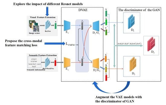
For zero-shot remote-sensing image scene classification, its purpose is to obtain a model trained from the image scenes of seen classes and use it to make correct predictions for unseen images. For this purpose, the cross-modal feature alignment method is used to train a model which projects both the visual features and semantic features of the image scenes into the latent space and make visual features in the latent space as close to their semantic features as possible. With the trained model, the visual features and semantic features of the image scenes of unseen classes can be also projected into the latent space. Then, in the latent space, a classifier will be trained with the generated semantic latent features which can classify the semantic latent features of different unseen classes. Because the visual features in the latent space are aligned with their semantic features, the classifier obtained can be also used to classify the visual features of unseen image scenes. In this way, the classes of the unseen image scenes can be predicted. The framework of the proposed method is illustrated in
Figure 1.
As shown in
Figure 1, the semantic information of unseen image scene classes are embedded with the NPL model such as Word2vec [
38] or Bert [
39] to obtain their semantic features
. Then
are mapped into the latent features
by the encoder
. At the same time, the image scenes are embedded with a pretrained feature extractor, such as ResNet18, to obtain their visual features
, which will be further mapped into the latent features
by the encoder
. In the latent space, the visual features
are aligned with their semantic features
. That is, the visual features
of each class are close to their sematic features
and far from those of other classes. Using the semantic features
, whose classes are known, a classifier can be trained. Since the visual features in the latent space are aligned with their semantic features, such a trained classifier can be also used to classify visual features and predict their classes.
It can be seen that the key of the cross-modal feature alignment method is to obtain the two modality encoders and which project the semantic features and visual features into the latent space, respectively, and make sure that they are aligned with each other. In this paper, we propose to integrate the VAE and GAN models to train such encoders. We detail the network architecture and the training process as follows.
3.2. The Network Architecture
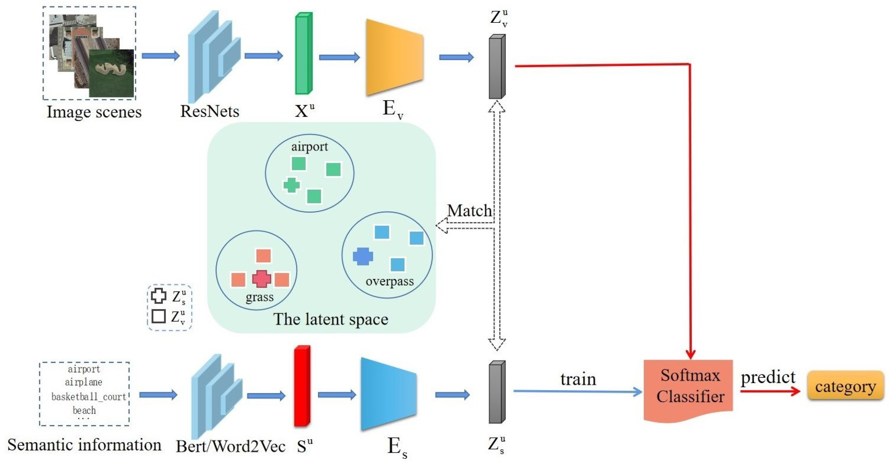
To obtain encoders which can project the visual and semantic features of image scenes into the latent space and make sure that they are aligned, this paper proposes to augment a VAE model with a GAN to integrate their strengths for better cross-modal feature alignment. The overall architecture of the integrated model can be seen in
Figure 2.
It can be seen that there are two main components in the model, namely, DVAE and Discriminator of GAN. With two different VAEs for different modalities, the DVAE is to project the visual features and semantic features of image scenes into the latent space and then reconstruct them. Each VAE consists of an encoder and a decoder. The encoders map the visual features and the semantic features of the image scenes into the latent space. Then, the decoders reconstruct the visual features and the semantic features from the mapped latent features. The two encoders are what we want, as shown in
Figure 1. In the meantime, there are three discriminators which measure the performance of the DVAE. The discriminators of
and
correspond to two VAEs, respectively, and the discriminator
is for both VAEs. Particularly, the decoder
and the discriminator
constitute a GAN in which the decoder
functions as the generator of the GAN. Similarly, the decoder
and the discriminator
constitute another GAN. In these GANs, the discriminators measure the quality of the reconstructed visual features and semantic features, and produce the probabilities that the reconstructed features are the original ones. Different from the discriminators of
and
, the input to the discriminator
are the cross-modal pairs of the visual features and the semantic features. It is to further judge whether the features in the pairs are the original ones or the reconstructed ones by measuring the compatibility or alignment between the cross-modal features.
Specifically, given a batch of image scenes, their visual features v and corresponding semantic features s are extracted in advance. Then, the encoders project them into the latent space. Following that, the mean and variance of the distributions of the visual features and the semantic features are estimated. They are the , , , and . Through sampling from the estimated distributions, the visual and semantic features and of the image scenes in the latent space are generated. For reconstruction purposes, the latent features of and will be input into the decoders and to obtain the reconstructed ones of and . For feature alignment purposes, the latent visual features will be input to the semantic decoder to obtain the new reconstructed semantic features . At the same time, the latent semantic features will be input into the visual decoder to obtain the new reconstructed visual features . Further, all the reconstructed visual and semantic features , , , and are input into the discriminators of and to predict the probabilities that the reconstructed features are the true features. For the discriminator , the visual-semantic pairs of (v,s), (v,), (v,), (,s), (,s) are input to predict the cross-modal matching degrees between the recontracted features and the true features.
Due to the application of the adversarial generative network, the proposed model will be trained step-by-step. That is, the discriminators are trained first in one epoch, and the DVAE is trained subsequently. The DVAE and the discriminators evolve through the adversarial learning. We detail the training process of the DVAE and the discriminators as follows.
3.3. The Training of DVAE
Given the visual and semantic features of the image scenes, the DVAE module maps the two modality features into the latent space and then reconstructs them. With the reconstructed visual and semantic features, the discriminators measure the effect of the reconstruction. In this process, the losses are computed for training the DVAE module. In the work of Schonfeld et al. [
15], three kinds of losses have been used. They are the VAE loss
, the cross-modal feature-reconstruction loss
, and the matching loss between the visual and semantic feature distribution in the latent space
. Besides these losses, another two kinds of losses are introduced in this paper. They are the adversarial loss
and the cross-modal feature matching loss
. The overall loss of the DVAE is defined as Equation (
3), where
is the weight factor of each kind of loss. We introduce these kinds of losses as follows.
3.3.1. The VAE Reconstruction Loss
The VAE reconstruction loss function used in this paper is defined as Equation (
4). It is the intrinsic loss function of the VAE model. By minimizing the VAE reconstruction loss, the reconstructed features are closer to the original features. In the definition,
denotes the data distribution generated by the encoder, and the
represents the data distribution generated by the decoder. In particular,
refers to the data distribution of the latent features
generated by the encoder
when given the visual features of
v.
3.3.2. The Cross-Modal Feature Reconstruction Loss
The definition of the cross-modal feature-reconstruction loss is shown in Equation (
5). Its purpose is to constrain two encoders to enable that their generated latent features to be aligned in the latent space. For this purpose, the latent semantic features are input into visual decoder to reconstruct the visual features, the latent visual features are input into semantic decoder to reconstruct the semantic features, and the distance between the reconstructed features and the original features are calculated as the loss. The
N denotes the number of training samples, and
and
represent the visual feature and semantic feature of i-th image scene.
3.3.3. The Feature-Distribution Matching Loss
The feature-distribution matching loss is also to enable the latent feature alignment by ensuring the cross-modal distribution alignment. Its definition is shown in Equation (
6), where
and
represent the the mean and standard deviation of the feature distribution in the latent space corresponding to i-th image scene. Specifically,
and
represent the mean and standard deviation of the distribution of visual feature.
3.3.4. The Adversarial Loss
The adversarial loss comes from the discriminators. When inputting the reconstructed features from the DVAE into the discriminators of
and
, we expect that the discriminators can’t recognize them as the reconstructed ones from the perspective of the decoders of
and
. This means that we expect them to predict the probabilities that the reconstructed features are the original ones as much as possible. Thus, the adversarial losses from the discriminators of
and
are defined as follows.
For the discriminator
, the inputs are the visual-semantic pairs of (
v,
), (
v,
), (
,
s), and (
,
s). We also expect that the discriminator will not recognize these input features as the reconstructed ones and predict the probabilities that the features are compatible as much as possible. Thus, the adversarial loss function for the discriminator of
is defined as follows.
Therefore, the total adversarial losses coming from the discriminators are as follows:
3.3.5. The Cross-Modal Feature Matching Loss
Considering the characteristics of intraclass differences and interclass similarities among the remote sensing image scenes, we introduce the cross-modal feature matching loss to further narrow the intraclass differences between the visual features and the semantic features of the same classes in the latent space, and enlarge the interclass distance between the visual features and the semantic features of different classes. The definition of the cross-modal feature matching loss is shown in Equation (
8) where
denotes the class of the i-th latent feature of
, and
means the matching metric of cosine distance.
is the number of the cross-modal feature pairs in which both the visual feature and the semantic feature come from the same classes. Meanwhile,
is the number of the cross-modal feature pairs in which the visual feature and the semantic feature are from different classes.
3.4. The Training of Discriminators
Once the visual features and the semantic features are reconstructed by the decoders of the VAEs, the discriminators measure the performance of the reconstructed features by judging whether there are reconstructed features in the inputs. Particularly, when training the discriminator of
, we input the original visual features
v and the reconstructed visual features
and
into the discriminator of
. And we expect that the discriminator has the ability to distinguish the reconstructed visual features
and
from the original visual features
v. That is, we expect that the discriminator produces the probability that the input features are the original ones as much as possible for
v, but, on the contrary, as small as possible for
and
. Thus, the loss function for the discriminator of
can be defined as follows.
Similarly, the loss function of the discriminator of
can be defined as follows.
For the discriminator of
, we will input the pairs of (
v,
s), (
v,
), (
v,
), (
,
s), and (
,
s) into it for training. The discriminator of
will produce the probabilities indicating whether there are reconstructed features in the pairs. Then, when inputting the pairs of (
v,
s), we expect that the discriminator of
predicts the portability as much as possible. In contrast, we expect that the discriminator of
predicts the probabilities as small as possible for these kinds of pairs of (
v,
), (
v,
), (
,
s), and (
,
s). Therefore, the loss function of the discriminator of
can be defined as follows:
Finally, the loss function for training these three discriminators is as follows:
4. Experiments
In this section, extensive experiments are conducted to evaluate the effectiveness of the proposed method by attempting to answer the following four research questions.
- RQ1.
How do the different kinds of losses defined in Equation (
3) contribute to model performance?
- RQ2.
Does the proposed method achieve better performance when compared with related methods?
- RQ3.
Does each improvement, i.e., the three discriminators and the cross-modal feature-matching loss, actually work as expected?
- RQ4.
What is the impact of different visual feature extractors on zero-shot image scene classifications performance?
4.1. Experimental Setup
4.1.1. Data for Experiments
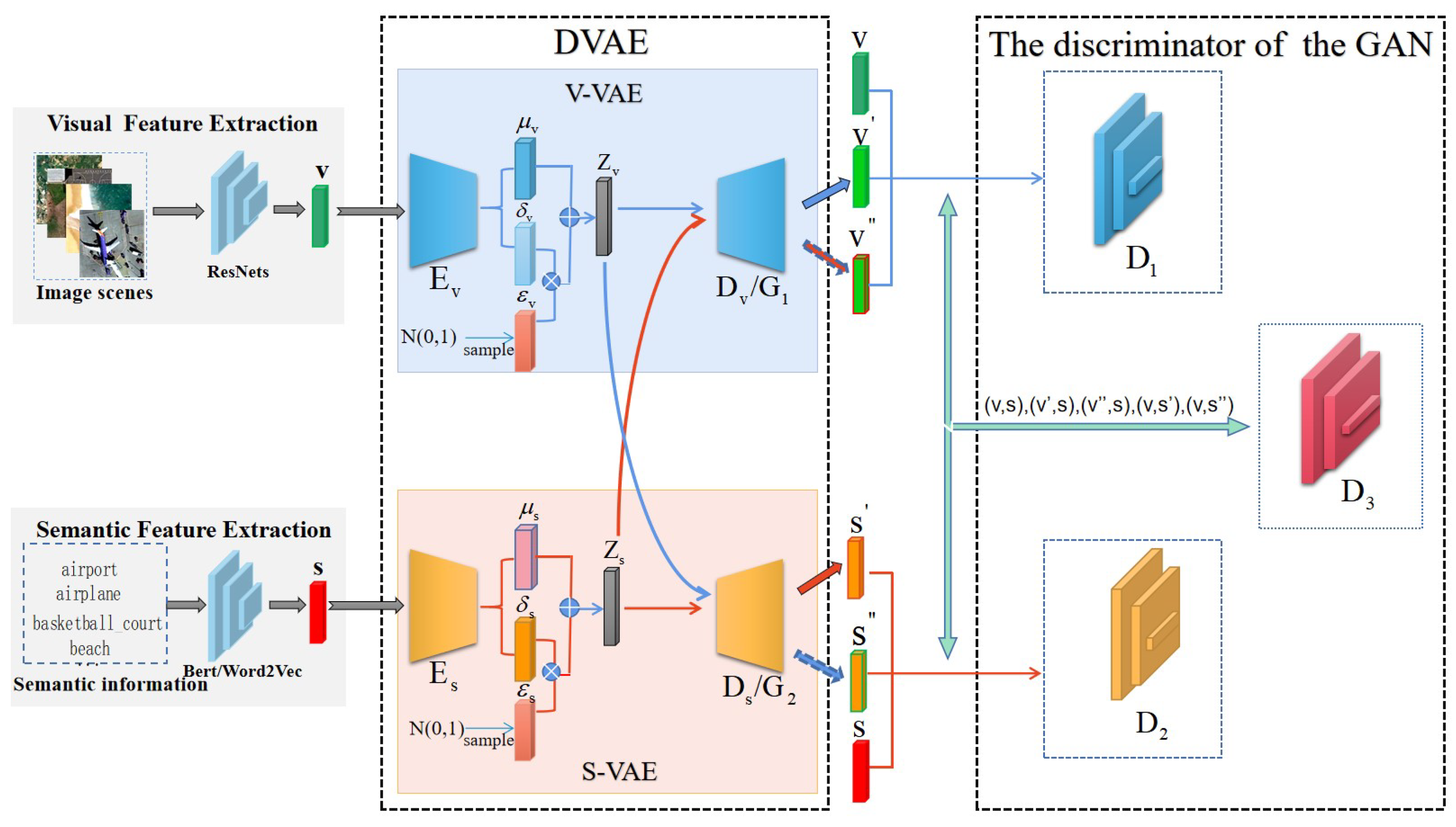
This paper takes the dataset which has been used in the work of Li, et al. [
19] for experiments. This dataset is the integration of five public remote sensing image scenes datasets including UCM [
40], AID [
41], NWPU-RESISC [
42], RSI-CB256 [
43], and PatternNet [
44]. The merged dataset realizes the complementarity between different classes and increases the diversity. This contributes to the validation of the zero-shot classification performance. There are 70 classes in the dataset, and 800 images with the size of 256 pixel × 256 pixel for each class. Some images of the dataset are shown in
Figure 3.
4.1.2. Metric of the Experiment
To measure the performance of the proposed method, this paper adopts the metric of overall accuracy (OA) which is defined as follows.
In the above equation, we adopt the widely used average per-class top-1 accuracy to evaluate the performance of each model where m represents the number of unseen classes. For each class of image scenes for testing, the accuracy is calculated by dividing the number of image scenes correctly classified by its total number of image scenes. The overall accuracy is the average of the accuracy of each class.
4.1.3. The Implementation
For the implementation of the proposed method, all the encoders and decoders are neural networks with only one layer. For the encoder and the decoder of the visual modality, their dimensions are set to 512. As the semantic feature dimension is smaller than that of visual features, the dimensions of the encoder and decoder for the semantic modality are set to 256. The discriminator
is designed as a neural network with only one hidden layer where the dimension is 1200. The discriminator
is also designed as a neural network with only one hidden layer where the dimension is 256. The discriminator
is designed as a neural network with two fully connected layers, where the dimensions are 1200 and 600. We set the batchsize to 50, the dimension of the latent feature vector to 32, and take 50 epochs to train the model. When using the generated latent semantic features to train a classifier for predicting the classes of unseen image scenes, the softmax classifier is applied. Our implementation is based on that of [
15].
We used the classical CNN backbone of the ResNet network, such as ResNet101, ResNet50, and ResNet18 models [
45], to extract the visual features of image scenes. They are pretrained on the ImageNet dataset. The 2048-dimensional features are extracted from the remote-sensing image scenes by using ResNet50 and ResNet101, and 512-dimensional features are there when using ResNet18. Regarding the extraction of semantic features, we adopted two kinds of sematic features used by the work of Li et al. [
19] for experiments, (1) the 300-dimensional features which are extracted from the class labels by using Word2Vec; (2) the 1024-dimensional features which are extracted by using BERT from a set of sentences describing the image scene classes.
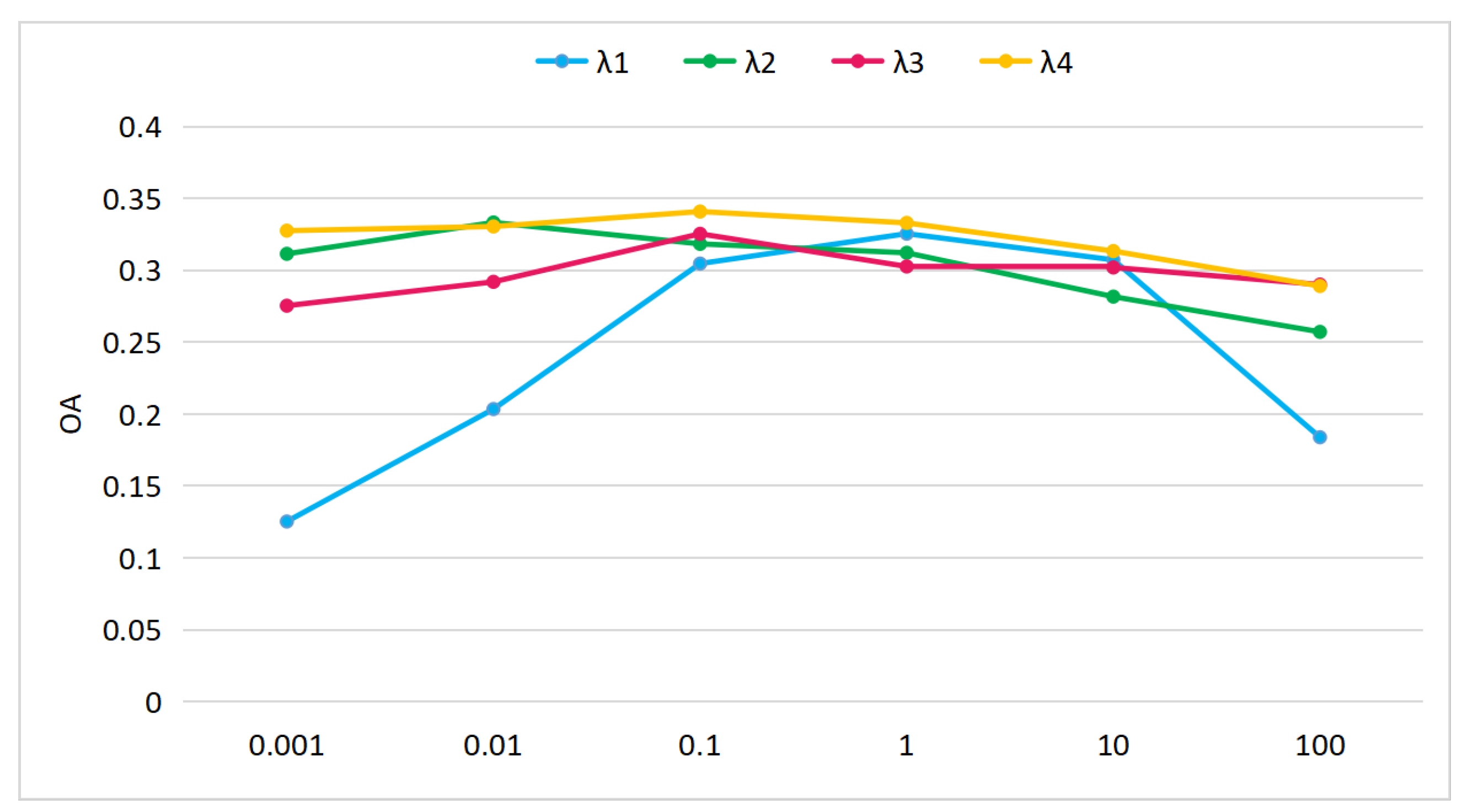
4.2. Hyperparameter Analysis
To evaluate the effect of the hyperparameters and answer RQ1, we analyzed the sensitivity of the hyperparameters of
,
,
, and
shown in Equation (
3). They are the weight factors of cross-modal feature reconstruction loss, feature-distribution-matching loss, adversarial loss, and cross-modal feature-matching loss. The experiment has been conducted under the seen/unseen ratio of 60/10, and the visual features from ResNet18 and the semantic features from Bert are adopted. The average of the classification accuracies over five random seen/unseen splits are recorded.
As shown in
Figure 4, while setting
,
, and
to 1, we tested the values in the set of
for
, and found that best performance was achieved when
. In the same way, we set
,
, and
as 1, our proposed method achieved the best performance when
. By setting
as 1,
as 0.01, and
as 1 to test the values of
, best performance was there when
. When testing the values of
, we set
as 1,
as 0.01, and
as 0.1, with the results indicating that it is better to set
to 0.1. Therefore, in our following experiments, we have set the hyperparameters of
,
,
, and
shown in Equation (
3) to 1, 0.01, 0.1, and 0.1, respectively.
4.3. Comparison with Related Methods
To validate the performance of our method and answer RQ2, we have compared it with several classical zero-shot methods. These methods include the embedding-based method of SPLE [
46] and the generative model-based methods of SAE [
23], CIZSL [
47], GDAN [
14], and CADA-VAE [
15]. SPLE [
46] introduced the idea of semantically preserving positional embedding, and achieved better matching between visual features and semantic features. SAE [
23] adopted the semantic feature representation as the hidden layer, and followed the AE model to learn the mapping from semantic space to visual space. CIZSL [
47] used generative adversarial network for zero-shot learning and introduced hallucinated text to the generator, encouraging the generated visual features to deviate from the seen classes and thus making the generated samples more diverse. GDAN [
14] built a dual generative adversarial networks and used dual adversarial loss and cycle consistency loss to bidirectionally map visual and semantic features. CADA-VAE [
15] proposed the construction of visual and semantic variational autoencoders to reconstruct features and align them in the latent space so that the constructed features contain basic multimodal information related to unseen classes. We have divided the dataset according to the ratios of 60/10, 50/20, and 40/30 to obtain the training set and the testing set. And both the semantic features from Word2vec and Bert are taken into consideration. The results of the comparison are shown in
Table 1.
As can be seen from
Table 1, our method achieved the optimal performance in most cases, which showed its effectiveness. Generally speaking, the embedding-based method of SPLE has not shown competitive performance when compared with these generative model-based methods. But, among these generative-based methods, the CIZSL method has the worst results. This may be because that the remote sensing image scenes are complex, usually containing a variety of objects. The generative adversarial network may not generate high-quality samples well due to its training instability, resulting in unsatisfactory ZSL classification results. Meanwhile, compared with the methods of SAE and GDAN, CADA-VAE has achieved better performance. This may be due to the fact that, unlike SAE and GDAN, CADA-VAE adopts the cross-modal latent feature alignment for zero-shot image scene classification instead of following the generative models to generate samples for unseen classes. Our method improved the CADA-VAE method by augmenting the VAEs with the discriminators of GAN, and the cross-modal feature matching loss. It can be seen that our method outperforms the CADA-VAE method, which validates the contribution of our improvements.
Moreover, when comparing the results under the semantic features from Word2vec and Bert, our method has better performance when adopting the semantic features from Bert, especially under the dividing ration of 60/10. This may be because that the semantic features from Bert with 1024 dimensions contain more information about the characteristics of image scenes. Further, similar to other methods, the proposed method obtained the best results under the dividing ratio of 60/10. This is because there are more classes for training and more knowledge can be leveraged for unseen classes.
4.4. Ablation Experiments
There are several new components (i.e., the discriminators of
,
,
, and the cross-modal matching loss) we have introduced, compared with the CADA-VAE method [
15]. To validate the benefits of these components so as to answer RQ3, we conducted ablation experiments by using semantic features from Bert. In the experiment, we have also validated the ways of dot production and Euclidean distance for calculating the cross-modal matching loss as well as the cosine distance. As shown in
Table 2, we have constructed the following model variants.
DVAE-DGAN augment the dual VAEs model with two discriminators of and , that is, equipping each VAE with one discriminator.
DVAE-GAN augment the dual VAEs model with one single cross-modal discriminator of for both VAEs.
DVAE-TGAN augment the dual VAEs model with all the discriminators of , , and .
DVAE-TGAN-, while adopting all the discriminators , , and , adopt the dot production to calculate the cross-modal matching loss.
DVAE-TGAN- while adopting the discriminators , , and , adopt the Euclidean distance to calculate the cross-modal matching loss.
DVAE-TGAN- while adopting the discriminators , , and , adopt the cosine distance to calculate the cross-modal matching loss.
It can be seen from
Table 2 that DVAE-TGAN achieves best result compared with the variants of DVAE-DGAN and DVAE-GAN. This shows the benefits of all these discriminators. When applying all these discriminators, more constraint information will be obtained. The constraint information can improve the encoders to better map the visual and semantic features of image scenes, and the decoders to better reconstruct them. Meanwhile, it is obvious that the strategy of equipping each VAE with a discriminator (i.e., DVAE-DGAN) is superior to that of applying a single cross-modal discriminator for both VAEs (i.e., DVAE-GAN). The reason may be that the different discriminators for different modalities will measure the reconstruction error more accurately than the cross-modal discriminator.
In addition, when comparing DVAE-TGAN with the variants of DVAE-TGAN-, DVAE-TGAN-, and DVAE-TGAN-, it can be seen that better performance is provided by the cross-modal feature-matching loss in most cases. This demonstrates the effectiveness of the cross-modal feature-matching loss. Among these methods of calculating the cross-modal feature-matching loss, it is better to use the cosine distance. This may be because it is better able to validate the alignment between the cross-modal features which are located in the high-dimensional space.
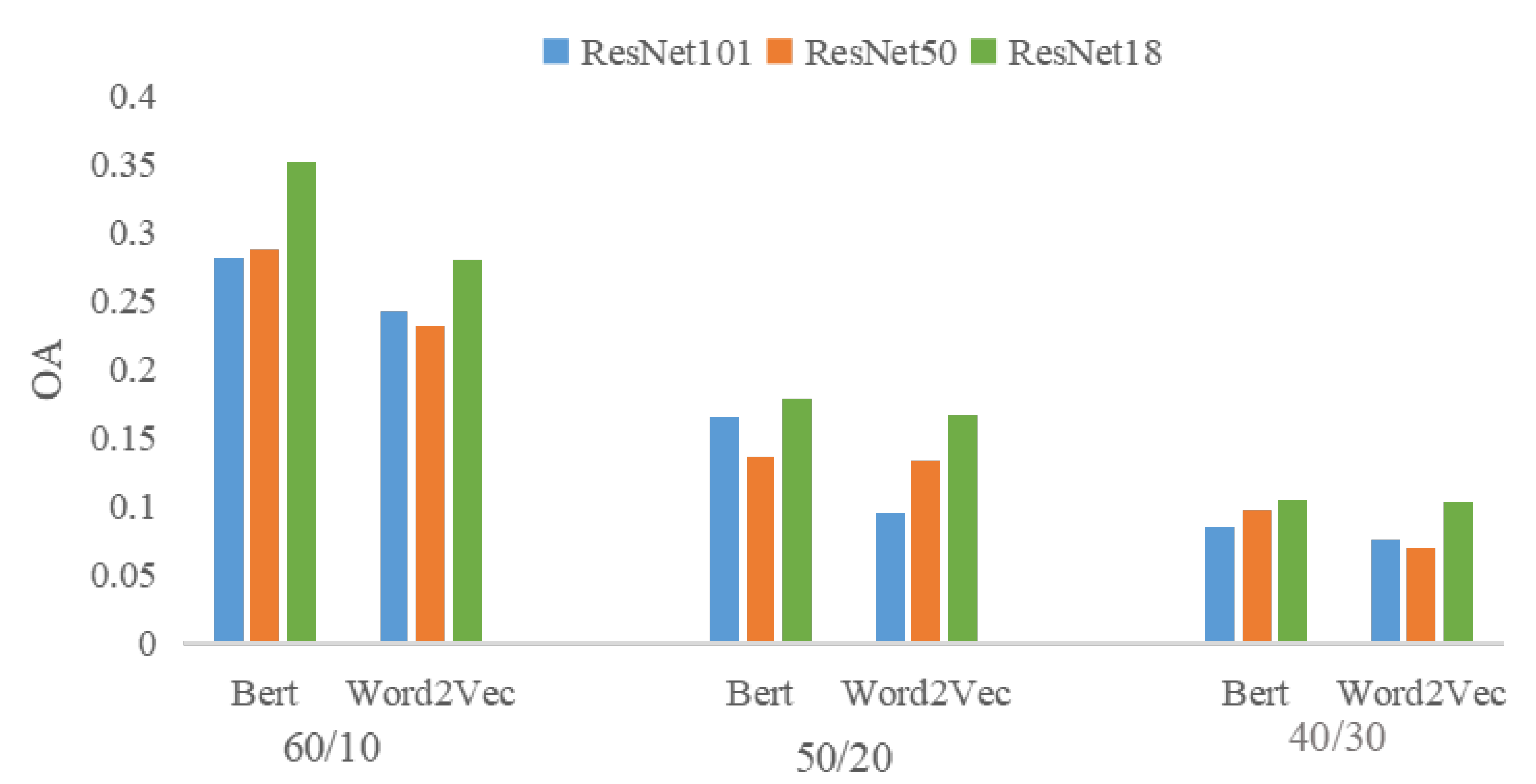
4.5. The Impact Evaluation of the Visual Feature Extractors
To achieve the cross-modal feature alignment in the latent space, the visual and semantic features are often extracted in advance by applying some extractors. It is obvious that these extractors play an important role for zero-shot image scene classification. The impact of the semantic feature extractors such as Word2Vec and Bert has been evaluated in related works. However, the impact of these visual feature extractors has not been investigated. Thus, taking the extractors of ResNet18, ResNet101 and ResNet50 as example, we have done an experiment to validate their different impact on our method and answer the research question RQ4.
Figure 5 shows the results of this experiment. It can be seen that for both two kinds of semantic features, better performance is there when ResNet18 is used as the visual feature extractor. In comparison, the features extracted by ResNet18 are smaller in dimension, i.e., 2048 dimensions for ResNet50 and ResNet101, and 512 dimensions for ResNet18. And from Resnet18 to Resnet50 and to Resnet101, there are more and more layers in each model. The results shown in
Figure 5 indicate that larger dimensions and more layers may not contribute to the image scene classification under a zero-shot setting. This may be because the shallow features will make a greater contribution to zero-shot image scene classification but are lost with the increase of layers.
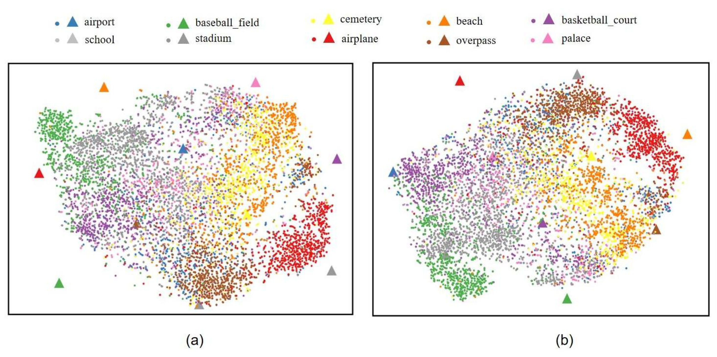
4.6. Visualization of the Latent Visual and Semantic Feature Alignment
The proposed method attempts to achieve better feature alignment between the visual and semantic modalities, that is, each class of visual features are closer to their own semantic feature and farther from other classes of semantic features. In order to provide a qualitative evaluation of the proposed method, we have visualized the latent visual and semantic features of the unseen image scenes to observe the cross-modal feature alignment in the latent space.
Figure 6 shows one of the results, where
Figure 6a is the visualization of cross-modal feature alignment without our improvements, while
Figure 6b is the visualization of the results of our method. Since there are more unseen classes under the seen/unseen ratios of 50/20 and 40/30, we have only used the latent features under the seen/unseen ratio of 60/10 for better visualization. Thus, there are 10 unseen classes of image scenes in the visualization. And there are 800 latent visual features (denoted by ⋅) and 1 latent semantic feature (denoted by ▲) for each unseen class. The original visual features of the image scenes are extracted by ResNet18 and the original semantic features are extracted by Bert. The tool of t-SNE [
48] is used for the cross-modal feature alignment visualization.
From
Figure 6a, we can see that the latent visual features of the classes of basketball _court (i.e., purple color), palace (i.e., pink color), and school (i.e., light grey color) are far apart from the latent semantic features of these classes. By comparison, as shown in
Figure 6b, the latent semantic features of these classes are surrounded by the latent visual features. In addition, it can be also seen that for the classes of baseball_field (i.e., green color), airplane (i.e., red color), and beach (i.e., orange color), the latent visual features become closer to the latent semantic features of their classes after applying the proposed method. But for the classes of airport (i.e., blue color) and overpass (i.e., khaki color), it seems that the latent visual features of these classes become further from the semantic features of these classes. On the whole, these visualization results also indicate the contribution of our proposed method to the cross-modal feature alignment.
5. Conclusions
This paper proposes augmentation of the dual VAEs with a GAN, for cross-modal feature alignment for zero-shot remote-sensing image scene classification. The concept is to make use of the GAN’s discriminator in order to learn a suitable reconstruction quality metric for the VAE. Given that there are two VAEs for the visual and semantic modalities, respectively, we propose to equip each VAE with a discriminator while adding another cross-modal discriminator for both VAEs. To promote feature alignment in the latent space and address the challenge of intraclass differences and interclass similarities, we have also proposed the cross-modal feature-matching loss to make sure that the visual features of one class are aligned with the semantic features of the class and unaligned with those of other classes. Based on the public dataset, our experiments have shown the contributions of the discriminators and the cross-modal feature-matching loss. In light of the fact that the visual and semantic features are often extracted in advance by applying some extractors and the impact of the different visual feature extractors has not been investigated, we have taken the ResNet models of ResNet18, extracting 512-dimensional visual features, and ResNet50 and ResNet101, both extracting 2048-dimensional visual features, for testing. The experimental results show that better performance is achieved by ResNet18, which indicates that more layers of the extractors and larger dimensions of the extracted features may not contribute to the image scene classification under zero-shot setting.


