1. Introduction
Highly populated urban areas are often critical for many aspects, like soil sealing and degradation, urban sprawl and, in general, loss of ecosystem services [
1]. GIS tools and spatial analysis have already demonstrated to be effective in urban planning [
2] and landscape evaluation [
3,
4,
5,
6]. In the last few years, the increasing number of free digital georeferenced data, especially remotely sensed ones, have started a new trend of spatial analysis for land planning and management, mainly relying on the exploitation of the time domain-related information that satellite missions can guarantee [
7,
8,
9]. The spatial distribution of environmental factors [
10,
11,
12], coupled with their dynamics along time, are expected to improve deductions especially about those territorial features showing a significant variability along time, i.e., vegetation.
Landscape metrics are already known to be effective in describing urban contexts [
13,
14,
15] and some experiences showed that the joint adoption of remote sensing data and socio-economic techniques [
16,
17] can significantly improve final deductions. In spite of a wide literature, in the most of cases, urban planning/management approaches rely on the interpretation of mere representations (maps) and, rarely, take into consideration quantitative concerns that are expected to increase the level of objectivity in urban reading, management and planning [
18,
19]. Within this general framework, in the climate change era, urban greenness is becoming a focus point in the public debate. Green areas, are, in fact, assigned, among the others, the role of mitigating the negative impacts of urbanization and creating more sustainable and healthier cities. Public or private vegetated areas—residential gardens, parks, street trees and surrounding natural areas—are known to provide benefits ranging from surface temperature reduction, air purification, noise mitigation, and promotion of physical/social activities and improvement of mental health [
20,
21].
Greenness is strictly related to vegetation phenology. Phenology describes periodic plant life cycle events across its growing season. Remotely sensed data have proved to be proper for monitoring macro-phenology, enabling the identification of significant markers along time series of maps of spectral indices.
Currently, phenology-related research in urban areas based on remotely sensed data focuses on many different types of applications. For example, urban phenology studies are retained useful to detect urban heat islands effects [
22] and to assess climate change impacts on urban vegetation [
23]. Other studies have investigated the impact of urbanization on vegetation phenology, highlighting its importance in defining proper strategies to mitigate negative environmental effects of urban growth [
24,
25]. Another important research area considers phenology patterns along urban-rural gradient [
26,
27] and, more in general, its impact on urban ecosystems [
28,
29]. The need of environmental compliant development and maintenance of contemporary cities is forcing this type of research, asking for sustainable solutions [
30]. The majority of these studies mainly rely on free and open medium/high resolution imagery. Data from the Landsat 8/9 and Sentinel 2 missions appear to be the most adopted ones [
21,
29,
31,
32], providing multispectral and multitemporal images with a GSD (Ground Sampling Distance) of 30 and 10 m, respectively, that is barely consistent with urban scale analysis.
Phenological studies can greatly support deductions related to the “greenness” of urban areas, moving from a static approach to a more dynamic one, where vegetation seasonal or inter annual processes can be easily described through the adoption of proper spectral (vegetation) indices [
31,
32,
33].
Traditional approaches to greenness were mainly based on subjective analyses based on personal perception and self-report methods involving question-based surveys. These were intended to investigate people feeling about vegetated areas fruition (e.g., access to parks) and their answers were analyzed by experts basing their deductions on specific a-priori defined criteria (e.g., presence/absence of various features) [
34].
Differently, remote sensing has introduced a more objective way of reading greenness. The majority of proposed methods rely on the adoption of various Vegetation Indices (VIs), like EVI (Enhanced Vegetation Index), NDVI (Normalized Difference Vegetation Index) and, more recently,
PPI (Plant Phenology Index) [
35].
When speaking about phenology as describable by satellite, one has to consider that it moves a little bit from its ordinary meaning. In fact, phenology should refer to a single vegetation species and should refer to a structured sequences of growing phases, often standardized by proper phenological scales (e.g., BBCH, [
36]). In the case of vegetation monitoring by remote sensing, it would be more appropriate to speak about macro-phenology, where a sort of both spatial and temporal “subsampling” of vegetation changes is operated. This result into a description of vegetation dynamics that refers to the average trends of groups of species through a temporal trend that moves according to the temporal resolution of the adopted satellite mission and of image availability (also depending on cloud coverage).
With these premises, approaches based on satellite data work on the analysis of local temporal profiles of spectral indices looking for synthetic markers that are generally referred as “phenological metrics” (PM). These refer to the time (along the year) and the strength of occurrences of particular markers (e.g., Start/End of Season, VI peak, profile steepness, etc.) [
37]. The spatial pattern of green areas is also considered when investigating urban greenness. The distance separating green spaces from urban suburbs, the number of green meters per inhabitant, the green space/built up area ratio and the percentage of green areas are typical space-related parameters.
The kind of vegetation may also vary within the same urban area and the possibility of mapping the related phenological differences is highly desirable for urban management and planning purposes. Deriving benefits may, in fact, be different for urban suburbs, in terms of both type and temporal duration of active vegetation along the year. With these premises, the traditional concept of greenness can be overcome and the temporal information introduced to somehow complete its meaning. Information about yearly persistence of vegetation and of its strength along the year is certainly useful to measure its potential effects, thus providing a new tool for completing the operational framework where urban planning strategies develop. Urban managers are, in fact, interested in exploring effectiveness of their management practices of green areas, and vegetation distribution and its behavior in terms of strength and duration is a type of information useful for programming requalification actions [
18,
38]. In the meantime this type of information can support modelling and assessment of vegetation-related effects on both reduction of the main air pollutants (e.g., PM10 and PM2.5, CO
2) and on allergological phenomena that are increasingly affecting urban population [
39,
40,
41,
42]. Additionally, vegetation mapping and its potential in improving population and town welfare is a worthy information that also economical players of the real estate market are interested about [
43,
44,
45].
In this framework, the time domain assumes a strategic role. In fact, the new need for urban planners is no longer classifying green areas, whose meaning and spatial distribution is already well known, but, conversely, to get the most of information about vegetation behavior along its growing season, to test the effectiveness of their choices, or calibrate the new ones for improving local welfare. This makes it definitely desirable to operate with remotely sensed data showing a high temporal resolution, possibly consistent with the growing times of vegetation. These requirements make Sentinel 2 data highly preferable with respect to the Landsat ones. Sentinel 2 images are, in fact, acquired with a temporal resolution of 5 days against the 16 from the Landsat one. Moreover, Sentinel 2 data have a GSD of 10 m against the 30 m of Landsat 8/9 one, making its image pixel geometrically consistent with the size of an adult tree canopy.
A second requirement from urban planners/managers is the easiness of interpretation and usage of information from remote sensing. In general, they are not properly skilled to process raw data and, consequently, remote sensing experts have to preventively prepare the information they need. Copernicus services move exactly along this direction and the HR-VPP (High Resolution—Vegetation Phenology and productivity) dataset is a first experience of data providing aimed at summarizing the most of information concerning vegetation behavior along time.
Looking at this general context, in this study, authors investigate limits and potentialities of the HR-VPP dataset in supporting urban planning and management, with special concerns about the increasing importance that, in the debate around climate change and sustainability of cities, greenness in urban areas is assuming. Specifically, greenness size, quality, and management are known to play an important role in supporting provision of ecosystem services to people within highly urbanized areas. It, directly, can provide services useful for human health like pollution reduction [
46], heat islands mitigation [
47], facilitation of people leisure related activities [
48], and aesthetical benefits [
49]. The possibility of continuously monitoring yearly vegetation dynamics is certainly a way for somehow quantifying and qualifying the supplying of the most of ecosystem services within the city, leading to immediately locate suffering areas in terms of both size and quality of the services themselves. Moreover, vegetation monitoring can indirectly inform about related (and complementary) natural components (i.e., soil and air) that can additionally provide ecosystem services to local population. This makes possible to link ecosystem processes to ecosystem services, as Fu et al. discussed in [
50].
It is worth highlighting that the main goal of this work is providing a sort of “how-to” for the exploitation of the new HR-VPP dataset in the specific context of urban management/planning with special concerns about requirements from Piemonte Region officers/technicians. Starting from the information that the HR-VPP dataset can provide, the authors draft a simple methodology for making the dataset itself closer to the final user, according to the users’ uptake policy of the Copernicus Program. No instance about validation of metrics is considered even if a preliminary test was done concerning the spatial consistence of the HR-VPP dataset. Most of the work was, conversely, aimed at proposing suggestions about the exploitation of this type of information through the integration with existing (and updated) official technical geodatabases.
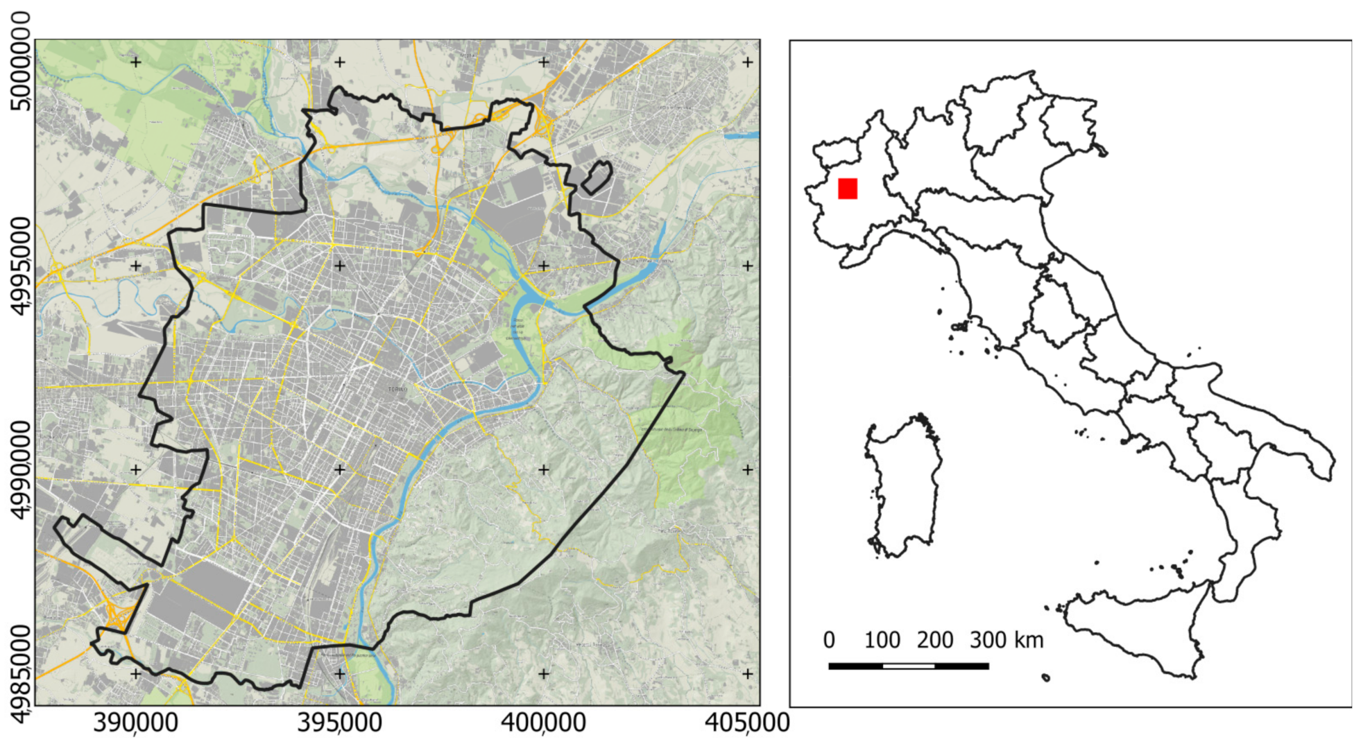
The study area corresponds to the municipality of Torino (NW, Italy), which is known to be one of the greenest cities in Europe.
A subset of the available phenological metrics from the HR-VPP dataset (namely the Length of the Season, LOS, and the Total Productivity, SPROD) were investigated by integration with the so called BDTRE dataset, corresponding to the vector implementation of the Piemonte Region official Geographic Database. SPROD and LOS were assumed as the most representative metrics useful in the urban planning/management context, somehow representing the strength of vegetative activity and its duration along the year, respectively (see forward on for more complete motivations about this choice). The study involved three years, namely, 2018, 2019, and 2020.
2. Materials and Methods
2.1. Study Area
The study area corresponds to the municipality of Torino, which is located in NW Italy and sizes about 130 km
2 (
Figure 1).
Located close to the Western Italian Alps, according to the Köppen Climate Classification (
https://www.weatherbase.com (accessed on 12 May 2022)), Torino presents a mid-latitude, four seasonal humid subtropical climate. Winters are moderately cold and dry; summers are mild over hills and quite hot in the plains. Rainfalls are frequent in spring and autumn, while during the hottest months, they are rare, but abundant, with frequent thunderstorms. Snowfalls are possible during winter months. Monthly average temperature ranges from −2.5 °C in winter up to 27.9 °C in summer.
Regarding morphological characterization, the territory of Torino presents altitude values ranging between 201 and 712 m.a.s.l., showing a variability proper of hilly territorial contexts. About 3000 ha of municipality, located in the south-west part of the study area, lay over hills.
The river system of Torino is made of four rivers: the Po river and three of its tributaries—Dora Riparia, Stura di Lanzo, and Sangone. Others minor water streams are: Gora Staretta, Ruscello Fracassa, Ruscello Sappone, and Ruscello Serralunga.
With regard to its green heritage, Torino is one of the greenest cities of Europe and it has been among the four finalists in the “European Green Capital 2022 Award” context (
https://environment.ec.europa.eu/topics/urban-environment/european-green-capital-award_en (accessed on 12 May 2022)) supported by the European Commission. It is worth reminding that the main goal of the context is to recognize and reward local efforts to improve environment, and thereby economy and quality of life within cities. The Award is assigned yearly to a city that proved to be excellent in promoting environmentally friendly urban living. Additionally, Torino has been, and currently still is, involved in several other initiatives that aim at building a sustainable and resilient city. Specifically, these projects and initiatives long for a sustainable management of green areas, and urban mobility; specific attention is paid to climate change effects with consequent and ad hoc urban planning solutions (
http://www.comune.torino.it/verdepubblico/ (accessed on 12 May 2022)).
2.2. Available Data: Official Technical Maps
The main land use classes adopted for this work were obtained from the BDTRE dataset [
51] updated at year 2019. BDTRE is a complete geodatabase, mapping technical features (buildings, roads, rivers, etc.) and thematic ones (cadastral, land use, building type, etc.) and represents the official cartographic reference for regional institutions and offices. BDTRE can be accessed and downloaded in vector format as Geopackage from the Geoportale of Piemonte Region (
https://www.geoportale.piemonte.it/cms/ (accessed on 13 May 2022)). The reference system of BDTRE is WGS84 UTM 32N and its nominal map scale is 1:10,000.
It is worth to remind that BDTRE is yearly updated. The choice of using the 2019 release (i.e., the intermediate year among the three considered ones) was made assuming that no significant change in urban green areas occurred one year before and one year later the 2019 mapped situation.
According to BDTRE, 34.2% of the whole urban context of Torino corresponds to green areas. The majority of these areas are urban parks and gardens, making up about 63% of the class. Woodlands make up about the 35% of the class: 92.6%, 1.42%, and 0.08% of woodlands correspond to broadleaves, shrubs, and conifers, respectively. The remaining 6% has no label assigned. Complete statistics can be found in
Table 1.
Concerning other classes, it can be noticed that: (i) agricultural areas size about the 8.44% of the study area and are mainly located in the peri-urban belt of the city; (ii) urbanized areas size about the 55.02% (75.87% built-up areas, 22.58% road network 1.53% sport areas). Within built-up areas, the majority of mapped polygons (64.95%) are labelled as mixed (residential and commercial), 12.29% as residential, and the 22.74% as non-residential. Water bodies cover about the 2.14% of the study area: 85.02% are rivers, the remaining 14.98% are lakes or ponds.
With reference to the above mentioned BDTRE classes, only the vegetated ones were considered for this work. To take care about planning instances from regional technicians, the native vegetation classes were aggregated considering their nature and use. The goal was to somehow differentiate natural vegetation (woodlands) from leisure-related managed vegetation (like parks and gardens), from agriculture-devoted areas and from fallow fields and pastures, that, due to the absence, or different, management, show a different macro-phenological behavior. According to these criteria 6 macro-classes were generated and used for the next analyses: (i) gardens and parks (i.e., private gardens and public parks), (ii) woodland, (iii) riparian formations, (iv) tree plantation, (v) fallow fields and pastures, and (vi) agricultural crops and arable land. They were summarized into a single polygon layer (hereinafter called C). The authors recognize that the class definition they used was something hybrid between land use and land cover. Nevertheless, the aggregated six classes appeared to be the most proper for satisfying needs from local urban planners.
2.3. Available Data: The Copernicus HR-VPP Product Suite
The HR-VPP product suite consists of the Vegetation Phenology Parameters, or Metrics, (VPPs) derived from the STs (Seasonal Trajectories) of the
PPI (Plant Phenology Index) index, on a yearly basis, after the end of the growing season.
PPI formulation was developed by Jin H. and Eklundh L. [
52] and is given in Equation (1)
where,
DVI is computed from sun-sensor geometry corrected red and NIR reflectances, K is a gain factor, M is a site-specific canopy maximum
DVI, and
DVIs is the
DVI of the soil. Please refer to [
52] for their estimations.
Metrics are derived by processing yearly Copernicus Sentinel-2 image time series having a nominal temporal resolution of 5 days. They are generated over the entire EEA39 region (33 member countries and 6 cooperating countries) and are available from the 2017 onwards, with yearly frequency [
53]. Thirteen VPPs metrics are provided for up to two growing seasons per year at pixel level with a GSD (Ground Sampling Distance) of 10 m. Metrics from HR-VPP data suite are reported in
Table 2. Theoretical specifications can be found in [
54].
It is worth reminding that, depending on the vegetated pixel, Season 1 and Season 2 can co-exist or not. Consequently, all vegetated pixels are characterized with metrics about Season 1, but for only few of them, the metrics of Season 2 can be provided.
It was not a goal of this work to validate HR-VPP metrics in terms of value. We, therefore, assumed as proper accuracy values reported in the HR-VPP User’s Manual [
54]. It textually reports that “
the accuracy of phenology metrics (SOSD, EOSD) as compared with ground observations shows a slight positive bias of 4 days for SOSD, and negative bias of −11 days (anticipated end of season) for EOSD. The shorter seasons is the main issue observed which was confirmed as compared to other datasets, resulting in a shorter length of the season of 15 (MR-VPP) and 36 (MCD12Q2) days. Users should consider with caution (due to a possible anticipation) the end of the season dates. Large variability can be found in phenology metrics for bare areas where no clear temporal variations are expected”.
According to the declared goals of this work, intended for suggesting an operational exploitation of the HR-VPP dataset useful for urban planning and management, only two metrics, out of 13, were considered for the analysis: the length of season (LOS) and the total productivity (SPROD). Additionally, the day of the start of season layer (SOSD) was also obtained for area masking purposes (see forward on). All the metrics were obtained for the Season 1 only. These metrics were selected according to the needs as expressed from urban planners, that appeared to be majorly interested in monitoring duration of greenness and biomass production as the most important metrics possibly dependent on their management actions. Other metrics, though scientifically important and crucial, were retained poorly dependent on local urban green management policies and, therefore, not considered in this work. Moreover, a simple and immediate information that can be easily interpreted by ordinary technicians, working in institutional offices, is mandatory. With these premises, selection of investigated metrics was done with no matter about scientific soundness of choice, but under the driving push of actual needs in urban management.
LOS,
SPROD, and SOSD metrics were downloaded from WEkEO, the EU’s Copernicus DIAS reference service for environmental data (
https://www.wekeo.eu/ (accessed on 13 May 2022)), through prior definition of the AOI for the years 2018, 2019, and 2020 for a total of six raster layers (ML).
2.4. Data Processing
2.4.1. Preliminary Quality Check of HR-VPP
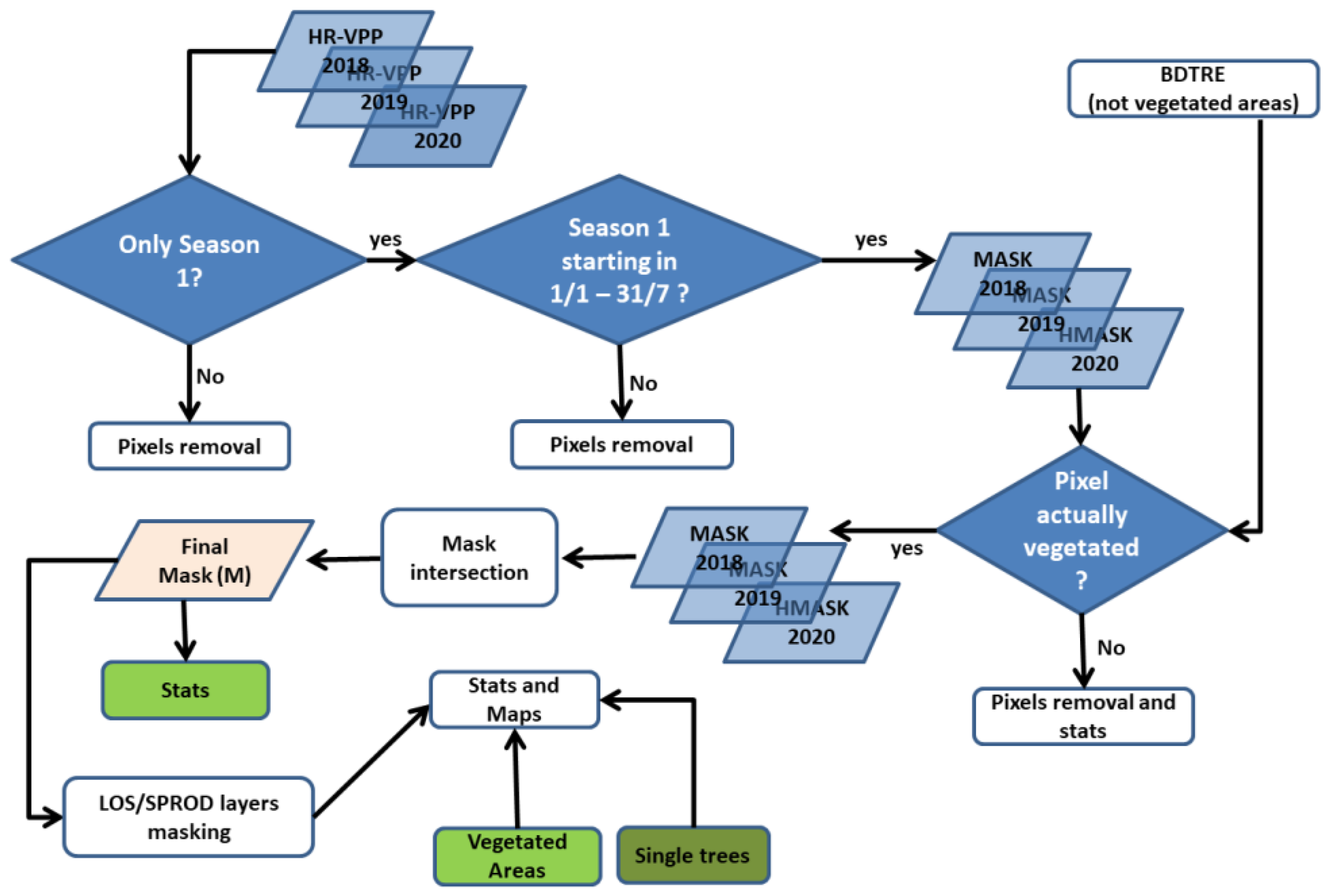
An important issue that had to be necessarily considered during data pre-processing was the one related to the possibility that the same vegetated area/point (as detected in HR-VPP) could show more than one growing season along the year (quite common in agricultural areas). Assuming that, in the area, only agricultural fields could show a second season and that urban green areas reasonably correspond to “natural” vegetation, only pixels showing a single season (i.e., Season 1) were considered. Moreover, only those pixels providing a SOSD metric of Season 1 ranging between DOY = 1 (i.e., 1 January) and DOY = 211 (i.e., 31 July) were selected. This choice was made despite the awareness of authors that peri-urban vegetation, often related to crops, could be of some importance in conditioning the overall picture of city vegetation. Three masks were, therefore, obtained for the three investigated years locating pixels that, according to HR-VPP dataset, were vegetated and showing a single phenological season along the year starting between 1 January and 31 July.
A first control was aimed at testing if these candidate pixels containing metrics, therefore mapped as “vegetated” in the HR-VPP dataset, were correctly corresponding to actual vegetated areas as mapped in the BDTRE. To test this condition, not vegetated patches (polygons) from BDTRE (complementary to C) were intersected by GIS tools (SAGA GIS v. 7.8.2, Olaf Conrad & Volker Wichmann, [
55]) with the above-mentioned masks and the number of pixels wrongly assigned counted. Some important inconsistencies, different depending on the year, were found (see Results and Discussions section).
Taking care about these tests, native masks were further refined excluding all those occurrences not corresponding to vegetated areas. Discrepancies among years were then investigated through comparison of yearly occurrences. Final masks (
My, one per year) were finally intersected to obtain a single one (namely, M) mapping all pixels verified as permanently vegetated along the three years. M was then used for masking
LOS and
SPROD layers, thus permitting to focus the analysis on those pixels reasonably associated to a vegetated element active for all the three investigated years. A synthetic flowchart is reported in
Figure 2.
A similar test was performed for single trees. The point layer T was compared with the yearly masks My to compute the number of trees properly/badly/missed detected in the HR-VPP dataset. This is a mandatory operation, being a single tree size barely consistent with HR-VPP GSD and, therefore, potentially not-detected at the spatial resolution of Sentinel 2 data. Again, statistics were generated for all the investigated years.
2.4.2. Per Class Phenological Metrics Analysis
According to the masked LOS and SPROD layers some descriptive statistics about area extent and number of patches were computed for the above-mentioned six macro-classes. Moreover, mean values of LOS and SPROD metrics were computed at vegetation macro class level for all the three investigated years and some summarizing statistics (namely, mean, standard deviation, and coefficient of variation along the years) interpreted.
Finally, LOS and SPROD mean values were computed at patch level by zonal statistics in SAGAGIS 8.1.1. on yearly basis, making possible to characterize all polygons of C with the correspondent mean value of both LOS and SPROD. These new attributes permitted to map local vegetation anomalies at polygon level for the three considered years that were useful to averagely read the local behavior of urban vegetation for planning/management purposes (see forward on).
2.4.3. Per Tree Phenological Metrics Analysis
As far as single trees characterization is concerned, points from T that properly corresponded to a filled pixel of HR-VPP dataset were firstly equipped with the correspondent LOS and SPROD metric value by extraction (nearest neighbor) from the correspondent raster layers.
Even though it contained a great variety of attributes that would have could be used to categorize tree point in T, the authors analyzed the entire dataset jointly to investigate the average behavior of trees in terms of LOS and SPROD, with no concerns about genus, categories or morphometric attributes.
For all the trees, the mean values of LOS and SPROD were, therefore, computed at year level and some synthetic statistics (namely, mean, standard deviation and coefficient of variation along the years) interpreted.
2.4.4. Interpreting Data for Understanding Urban Greening
Trying to synthesize the enormous content of the HR-VPP dataset and moving to its exploitation in terms of urban planning and management, all the above-mentioned macro-classes from C were considered and LOS and SPROD class metrics separately analyzed for the 3 years. In particular, the focus was on mapping positive and negative anomalies of vegetation behavior over Torino in terms of both yearly duration (LOS) and potential biomass expression (SPROD) with the aim of somehow mapping the potentiality of local greenness to improve citizens’ wellbeing: the higher the yearly duration and biomass expression of vegetation, the higher the expected benefits for local population. An inter-annual comparison of anomalies was also achieved to test the degree of persistence of local yearly anomalies.
Anomalies were computed according to Equations (2) and (3), for
LOS and
SPROD, respectively.
where
SPRODi and
LOSi are the local average patch values of
SPROD and
LOS, respectively;
and
are the mean metric values from all vegetated areas (independently from the class).
LOS and SPROD anomaly assessment, aimed at suggesting operational approaches for HR-VPP data exploitation in the urban planning/management context, was achieved with reference to C solely, retaining an at-patch level analysis more effective and exhaustive than one based on point features (trees) that, however, can be eventually recovered for further future and more specific refinements. Results concerning single tree characterization, at this point and for the goals of this work, are just intended to preliminary demonstrate the properness of LOS and SPROD from HR-VPP dataset, in describing their phenological behavior.
3. Results and Discussions
3.1. Preliminary Quality Check of HR-VPP
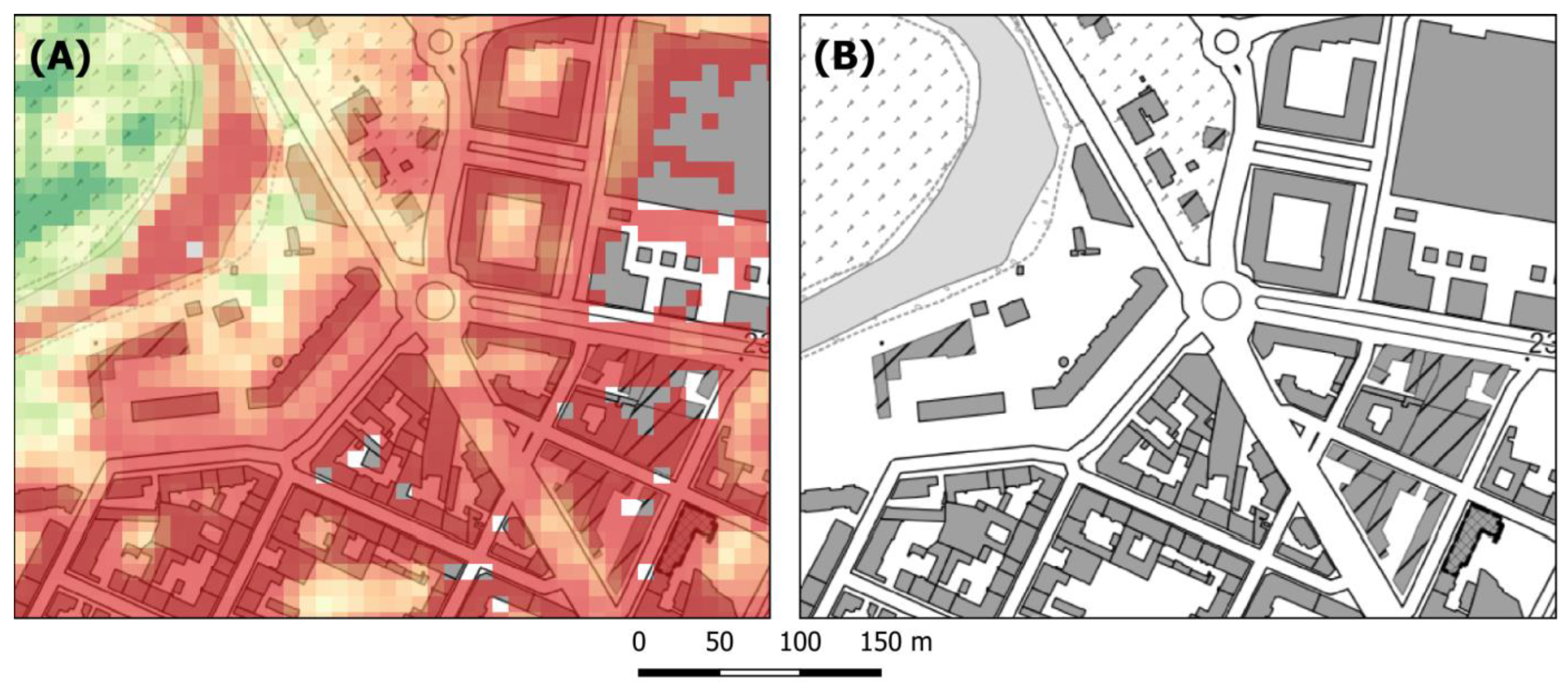
A first investigation concerned the spatial consistence of vegetated pixels from HR-VPP with vegetated elements as mapped in the BDTRE. The yearly masks were used for this purpose. They were tested against the not-vegetated patches obtained from the BDTRE. A high degree of overestimation was found by HR-VPP in terms of vegetated pixels for all the years. In particular, it was found that 51.97% (2018), 52.43% (2019), and 53.20% (2020) of vegetated pixels in HR-VPP corresponded to different classes of BDTRE in the investigated years. Some evidence is shown as an example in
Figure 3.
A second investigation concerned the comparison between yearly masks generated considering the above-mentioned criteria: (i) only pixels with a single season starting between 1 January (DOY = 1) and 31 July (DOY = 211); (ii) only pixels corresponding to vegetated element as mapped in C or T.
This analysis was aimed at testing the percentage of vegetated pixels yearly active along all the three investigated growing seasons (2018, 2019, and 2020). It was found that the 86.90% of pixels remained vegetated for all the three investigated years confirming a significant stability of vegetation presence in the area. Only the 8.0% and 5.1% of pixels were mapped as vegetated for only 2 or 1 years, respectively.
Only pixels that showed to be recognized as vegetated for all the three years and corresponding to actual vegetated areas as mapped in BDTRE were considered to generate the final mask M used for the next analyses.
As far as single trees from T are concerned (108,055 in the municipality of Torino), it was found that for only 1325 out of them (about 1.2%), it was not possible to associate the correspondent phenological metrics from HR-VPP. This means that for the remaining 98.8% of trees the corresponding metrics were available.
Moreover, while testing occurrences of the Season 2 for trees (expectation was that trees show one season only), unexpectedly, it was found that 24.37%, 30.25%, and 22.43% of trees showed metrics of Season 2 for 2018, 2019, and 2020, respectively.
3.2. Per Class Phenological Metrics Analysis
To recover the operational meaning in the urban planning/management context,
LOS and
SPROD metrics were used to characterize, along the 3 years, green areas in Torino. A first type of information one has to consider is the one related to the spatial distribution of vegetated (macro-) classes over the area.
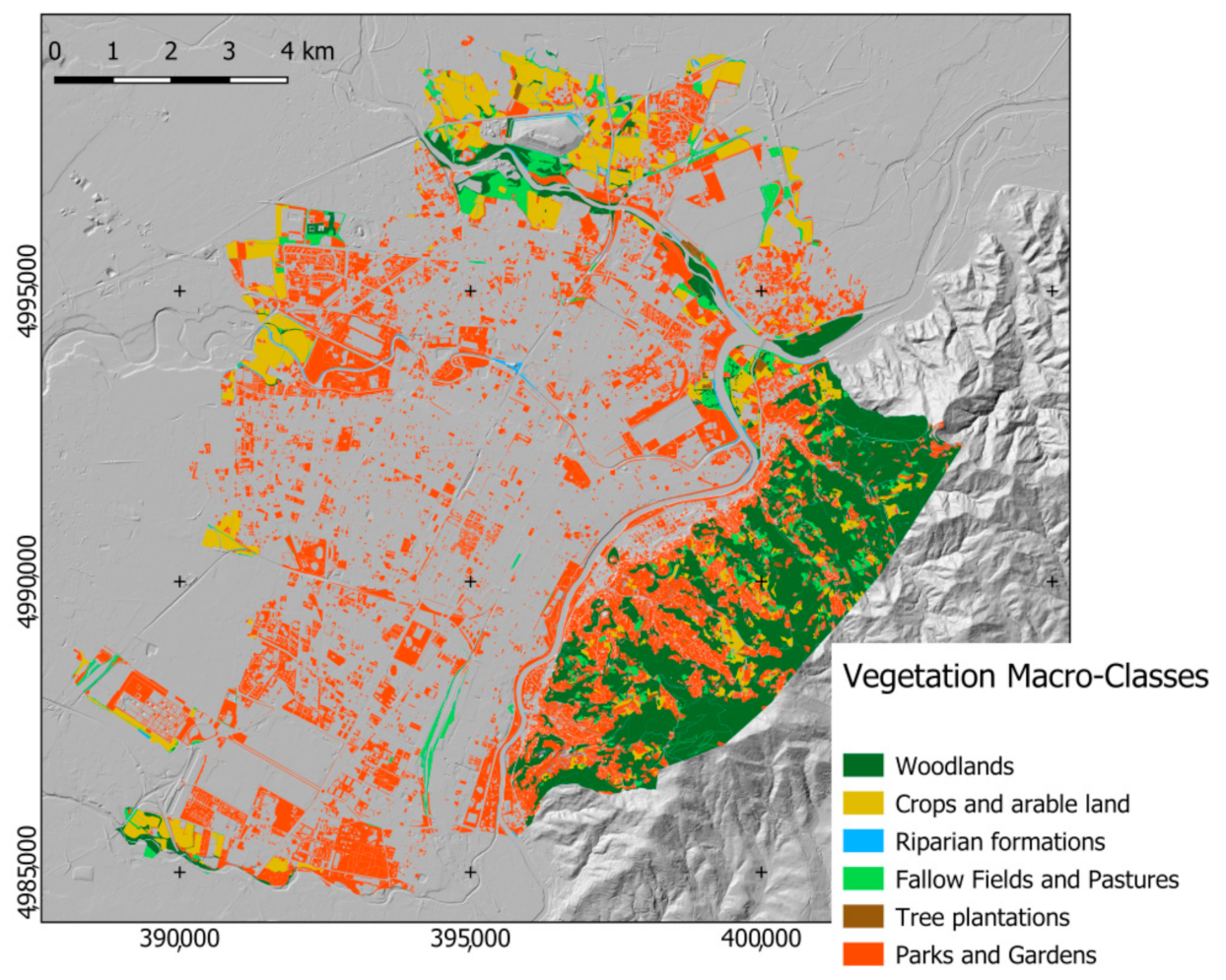
Figure 4 shows the spatial consistence and distribution of the vegetation macro-classes of the C layer.
Table 3 reports some statistics concerning geometric features of the vegetation classes as mapped in C, where it can be noticed that gardens and parks are largely the prevailing urban green areas sizing about the 50% of the total.
The hilly area located in the South-Eastern part of the city, beyond the Po River, hosts the most of woodlands (about 28% of urban green areas). Crops and pastures jointly capitalize about the 20%, reminding about the great importance that, still today, agriculture plays in the urban fringe of the metropolitan area. These areas are mainly located in the flat peri-urban belt of the city (mainly western ward), but some remainders can be found on the hill, where woodlands enormously prevail. Even if agriculture-devoted patches would require a deeper analysis from the phenological point of view, being exactly the ones that possibly express two yearly growing seasons, they are retained marginal for the goals of this work and, therefore, no further investigation is given.
As far as phenological behavior of these areas is concerned,
LOS and
SPROD yearly class mean values were computed and reported in
Table 4.
It can be noticed that the average duration of vegetation (LOS) in the area is half a year (about 180 days) for all the classes with an inter-annual variability from 5 to 8 days (LOS standard deviation). Nevertheless, patches corresponding to tree plantations show, averagely, a duration up to 10 days longer than the others, possibly depending on management practices.
Interesting considerations can be made if looking at SPROD. Tree-related classes show significantly higher SPROD values, confirming that the algorithm behind the HR-VPP dataset works well, correctly detecting a higher biomass production (about + 14% per year) in forested or tree-populated areas.
Additionally, SPROD value corresponding to the garden and parks class ensures about the idea that HR-VPP estimates are, at least relatively, reasonable. In fact, this appears to be averagely 45% lower of the other classes confirming that, these areas are constantly managed by cuts and biomass removal.
3.3. Per Tree Phenological Metrics Analysis
After removing from T all those trees that could not be associated to a filled pixel from HR-VPP dataset for all the three years, 106,730 trees remained out of the initial 108,055. These were used to preliminary test the capability of HR-VPP dataset of characterizing their behavior in terms of
LOS and
SPROD. Some statistics (
Table 5) were extracted with no concern about tree genus.
Comparing metrics estimates as computed at area (from C layer) and tree (from T layer) level, we can derive the following: (i) at-tree and at-patch level LOS mean values are consistent; consequently, the description of the time of macro-phenology by HR-VPP at both patch and single tree level can be assumed as reasonably reliable; (ii) SPROD as estimated at patch level appears to be significantly higher (about + 63%) than the one from trees. This can be related to the background effect, possibly affecting estimates at tree level, that reasonably are derived from not-pure pixels resulting from the joint spectral contribution of tree canopy and urban materials of roads/buildings surrounding the tree; (iii) similarly, the coefficient of variation (along time) appears to be similar for single tree and forest patches for LOS (around 3.7%) and significantly different for SPROD, confirming that SPROD estimates at single tree level could be somehow unreliable.
3.4. Interpreting Data for Understanding Urban Greening
To better characterize and summarize macro-phenological behavior of vegetated areas in Torino, LOS and SPROD anomalies were computed according to Equations (2) and (3), and mapped. Reference mean value for anomaly computation is the one from all the patches, independently from the vegetation class.
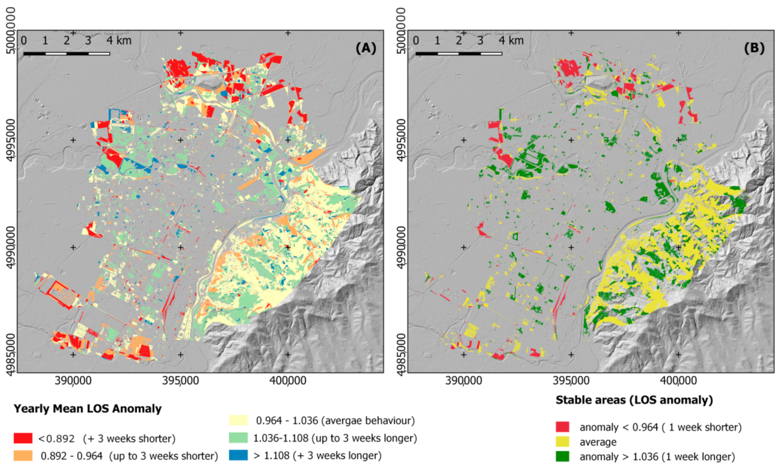
3.4.1. Analyzing LOS
Figure 5A shows the spatial distribution of the average
LOS anomalies resulting by averaging the three yearly values. Five classes were mapped: (i) one mapping patches showing an average
LOS anomaly < 0.0892 corresponding to those areas where the growing season is somehow shorter more than 3 weeks with respect to the mean; (ii) one mapping patches having a growing season shorter up to 3 weeks with respect to the mean (0.892–0.964); (iii) one mapping patches having an average growing season (0.964–1.036); (iv) one mapping patches having a growing season longer up to 3 weeks with respect to the mean (1.036–1.108); and (v) one mapping patches having a growing season longer more than 3 weeks with respect to the mean (>1.108).
Figure 5B, differently, is intended to show those patches that constantly behave along the three investigated years always over, under or similar to the yearly mean value of
LOS. In other words, those vegetated patches that constantly show a shorter, longer, or average duration of their growing season. In
Table 5, some summarizing statistics are reported.
Table 6 shows that: (i) about the 50% of the vegetated area of Torino show a stable behavior in terms of
LOS anomaly along the three investigated years, always vegetating shorter, longer or similar to the local average
LOS value (
Figure 5B); (ii) class 2 shows the averagely greater patch size (about 2 ha) that majorly correspond to the hilly forested area, i.e., the most natural one.
Table 7 shows that the most stable vegetation type in terms of
LOS is the mostly managed one intended for aesthetical/leisure purposes, i.e., gardens and parks. It absorbs the 44.13% of “stable” areas showing a dominance of classes 2 and 3; this demonstrates that management practices (public or private) induce a longer green staying along the year for these areas, thus improving their beneficial effects for populations.
It is also remarkable that the most stable vegetation in terms of average LOS is the one of woodlands, i.e., natural vegetation, that possibly traces the average yearly phenological behavior of local vegetation. As further evidence of these metrics, crops and arable lands show a prevalence of the class 1, i.e., the one corresponding to averagely shorter growing seasons; these values are highly reasonable if thinking about the ordinary macro-phenology of crops, that is generally and suddenly interrupted by harvest. All these facts ensure about LOS metrics from HR-VPP, suggesting that, at least relatively, they well fit local conditions.
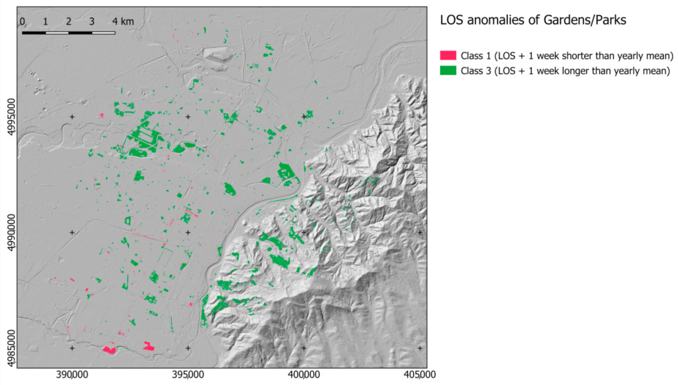
While focusing on parks/garden class (
Figure 6), it can be noted that the most of patches (about 92%) shows a positive
LOS anomaly, while only a minority has a negative one, i.e.,
LOS value shorter than yearly mean. This can be interpreted as a result of the good ordinary management practices for public green areas exploited by the municipality administration. Moreover, spatial distribution of patches of
LOS positive class is uniformly spread within the city, suggesting that management practices are more conditioning
LOS than vegetation type and local urban conditions. This ensures longer lasting beneficious effects provided by active vegetation to citizens.
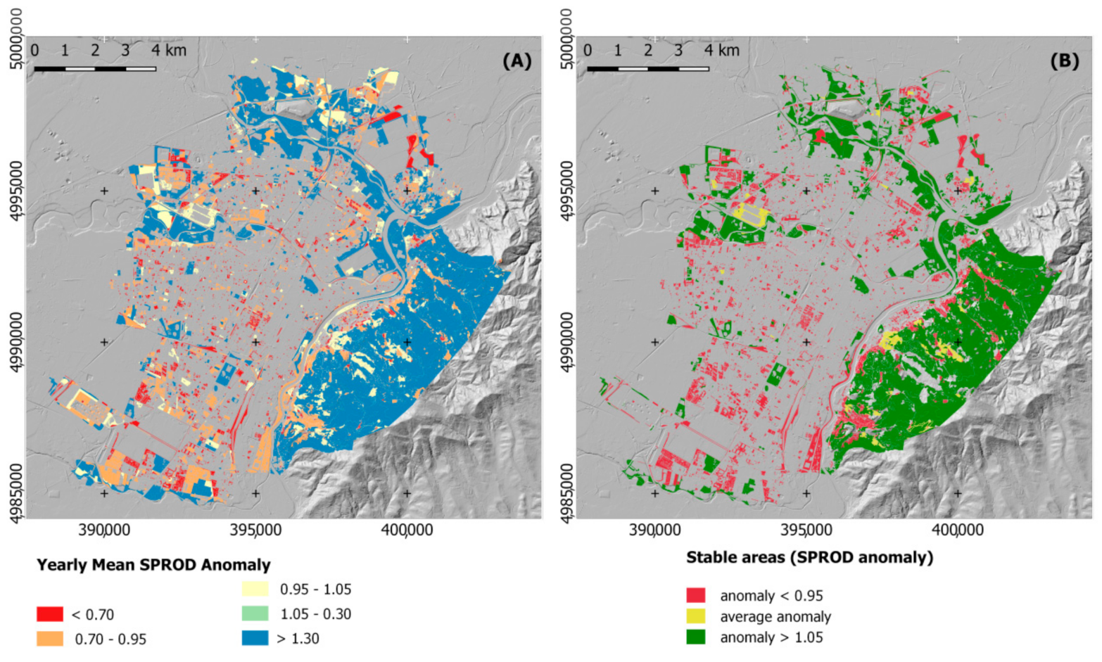
3.4.2. Analyzing SPROD
Figure 7A shows the spatial distribution of the average
SPROD anomalies resulting by averaging the three yearly values. Five classes were mapped: (i) one mapping patches showing an average
SPROD anomaly < 0.7, corresponding to those areas where total productivity is somehow smaller more than 30% with respect to the mean; (ii) one mapping patches having a total productivity smaller up to the 30% with respect to the mean (0.7–0.95); (iii) one mapping patches having an average total productivity (0.95–1.05); (iv) one mapping patches having a total productivity bigger up to the 30% with respect to the mean (1.05–1.3); and (v) one mapping patches having a total productivity bigger more than 30% with respect to the mean (>1.108).
Figure 7B, differently, is intended to show those patches that constantly along the three investigated years always show bigger, smaller, or similar
SPROD value with respect to the yearly mean.
Results from
Table 8 and
Table 9 show that the
SPROD mean value, computed without considering the vegetation type, is poorly significant, since class 2 (vegetation showing a stable behavior around the mean) just represent the 3% of the total.
Class 3 (vegetation showing a productivity significantly higher than the mean) is the most frequent one and it majorly corresponds to forests, immediately followed by garden/parks (
Table 9). This finding is highly encouraging regarding the robustness of the
SPROD estimates, since classes that were expected to provide the highest biomass production (woodlands and forested parks) are the most recurrent ones in class 3.
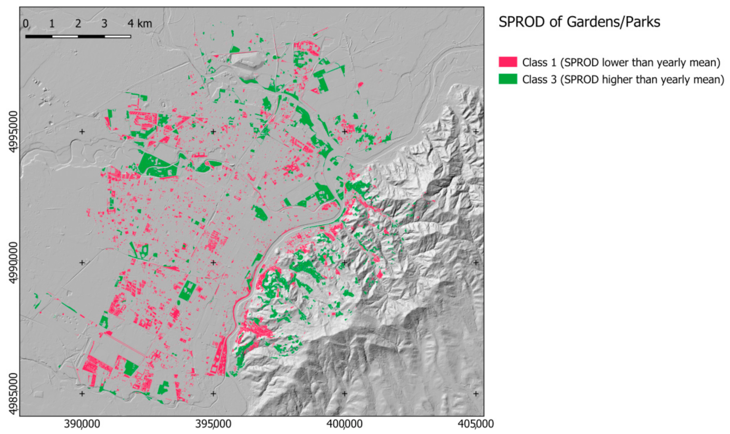
With a further specific focus on the only urban green (i.e., gardens/parks class), the analysis showed that patches are almost equally balanced in term of anomalies of biomass production, with almost half of patches having
SPROD anomalies lower than the yearly mean and remaining half with
SPROD higher than the same value. Regarding spatial distribution of
SPROD anomalies classes, these are uniformly distributed, and no remarkable differences can be observed; there is no specific area of the city characterized by more or less biomass production then another one (see
Figure 8), and, consequently, no specific part of the city benefits more then another one of resulting benefits.
4. Conclusions
In this study, the authors have proposed a simple methodology to translate phenological metrics into planning/management concepts starting from requirements of the regional officers/technicians. A first concern was the one related to the selection of proper and immediate metrics from the whole HR-VPP dataset. SPROD and LOS were assumed as the most representative ones to face urban planning/management instances, somehow representing the strength of vegetative activity and its duration along the year, respectively. With reference to these metrics, the authors have, initially, tested their spatial consistency with the BDTRE reference map by comparing vegetated areas from HR-VPP dataset (i.e., pixels containing metric estimates) with the BDTRE ones. The comparison involved two types of features: (i) areal ones, corresponding to vegetated patches as mapped in the BDTRE regional geodatabase; and (ii) point ones, corresponding to single trees as mapped in the available official WFS layer from the Torino Municipality administration.
As far as spatial consistency was concerned, it was found that HR-VPP dataset greatly overestimates (about 50%) vegetated areas in the city, assigning metric values to pixels that, if compared with technical maps, do not fall within vegetated areas. This probably depends on the high number of occurrences of shadowy areas that, possibly, introduces some noise during data processing, that algorithms cannot properly manage.
Concerning interpretation of metrics, it was found that LOS and SPROD well describe the behavior of vegetated areas, making possible to properly zone the city and make management of green areas and real estate considerations more effective.
Differently, only LOS proved to be able to reasonably describe the behavior of single trees; corresponding SPROD values, in fact, proved to be significantly lower of the expected values, suggesting that, only HR-VPP metrics aimed at describing the “times” of the growing season can be somehow exploited at single tree level. Conversely, all those quantitative metrics aimed at measuring the “strength” (biomass, vigor, etc.) of macro-phenological events cannot be properly associated to single trees.
Among the proposed approaches aimed to translate phenological metrics into planning/management concepts, LOS and SPROD anomalies were then mapped for the considered macro classes, in order to provide a zoning of the city based on positive or negative anomalies with respect to the yearly mean class behavior.
As expected, woodlands represented the best class in term of biomass production, making quite attractive the surroundings urbanized areas in term of linked benefits on health and on life quality more in general.
On the contrary, classes like tree plantations, riparian formations and pastures were, as expected, least significant in term of duration and strength of vegetation, making the urbanized neighboring areas less tempting from the health benefits point of view.
A specific focus was done on gardens and parks. It was noticed that the majority of patches shows longer LOS, probably thanks to the ordinary good management practices operated by the municipality administration. No remarkable finding, useful to improve management, was obtained about the spatial distribution of LOS and SPROD anomalies of parks and gardens, showing that there is no specific part of the city that benefits more than another in term of season length or of biomass production.
An important information was the one related to the location of those patches showing a significantly shorter LOS and/or lower SPROD; this is an important input for the municipality administration to properly plan the management of these green areas, aiming at their improvement from a phenological point of view through a prioritized approach. Ad hoc management practices would contribute to raise the value of the neighboring urbanized areas in term of linked benefits on life quality, with direct effect in the real estate market.


