

Mitigating Effect of Urban Green Spaces on Surface Urban Heat Island during Summer Period on an Example of a Medium Size Town of Zvolen, Slovakia

Abstract
:
1. Introduction
2. Materials and Methods
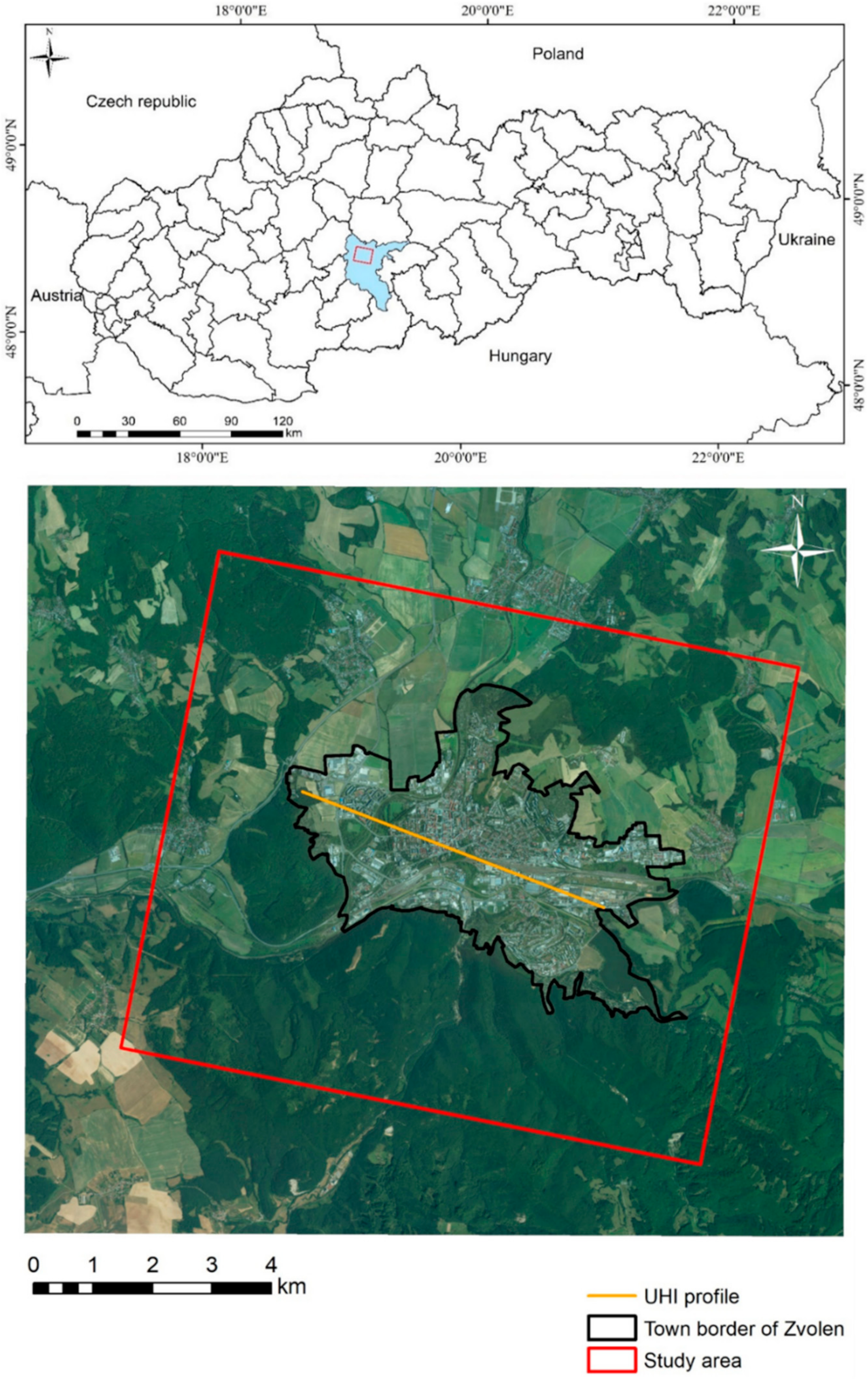
2.1. Study Area
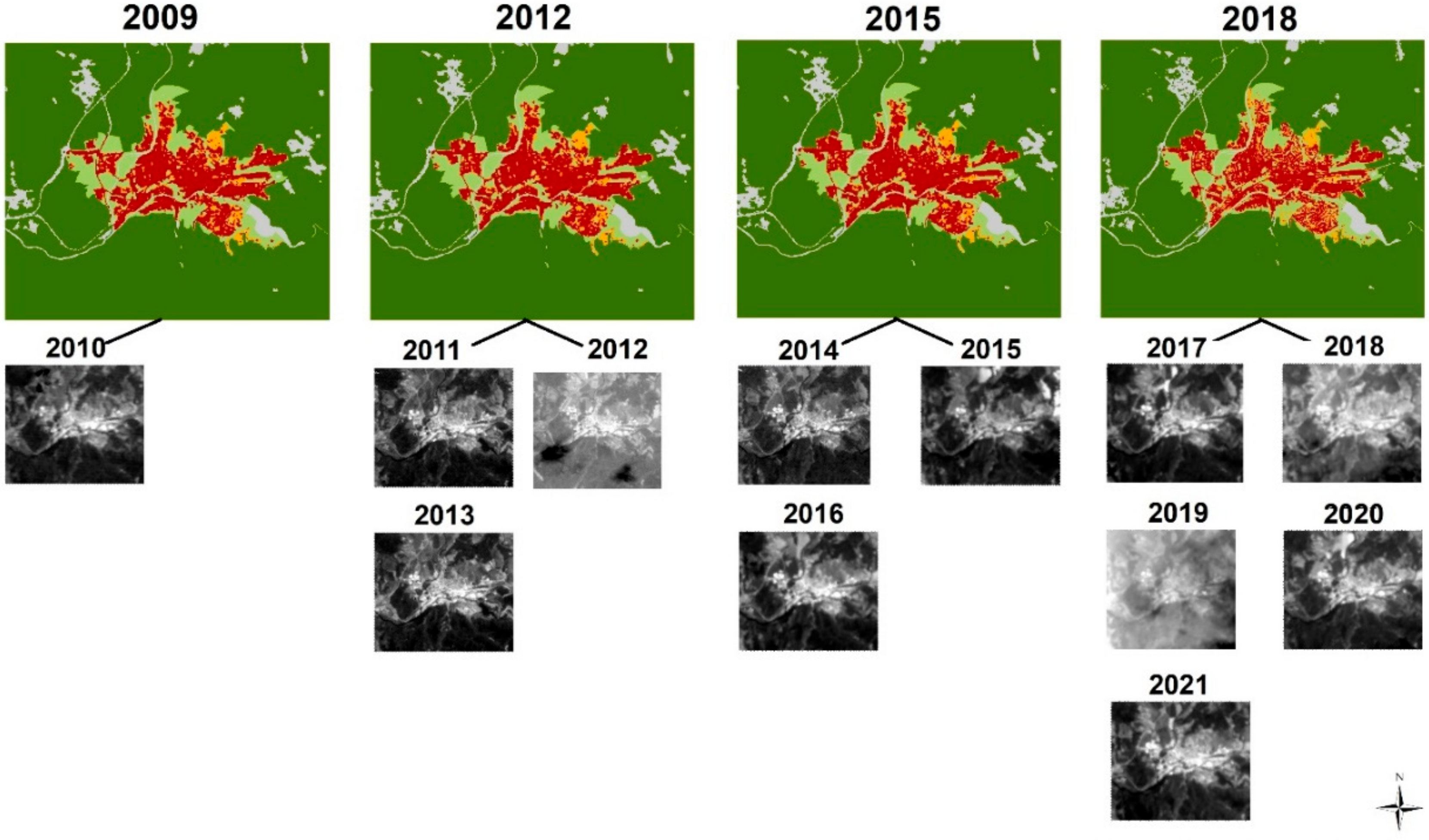
2.2. Data Sources
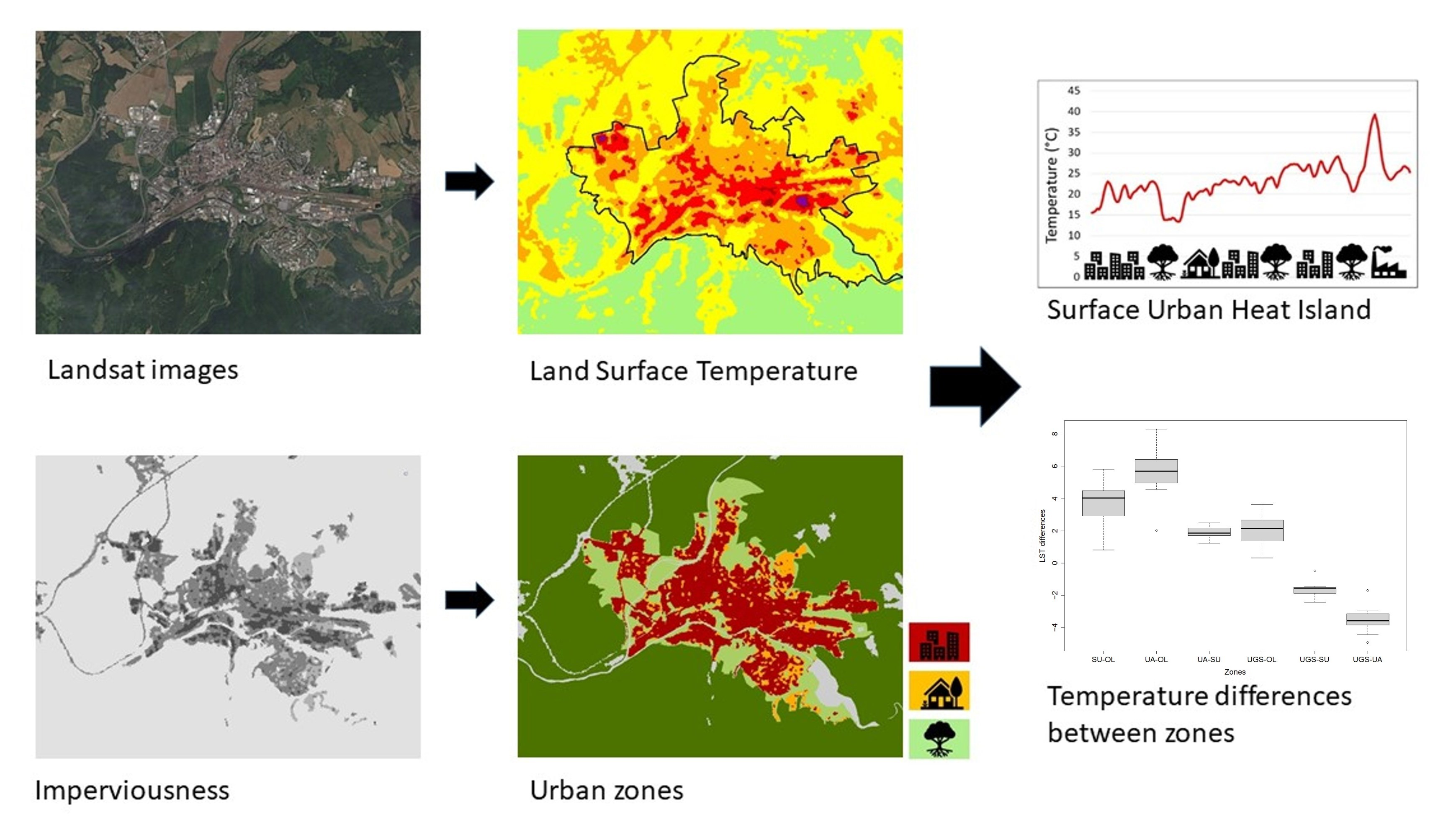
2.3. Land Surface Temperature Retrieval
2.4. Urban Heat Island and Urban Heat Island Intensity Retrieval
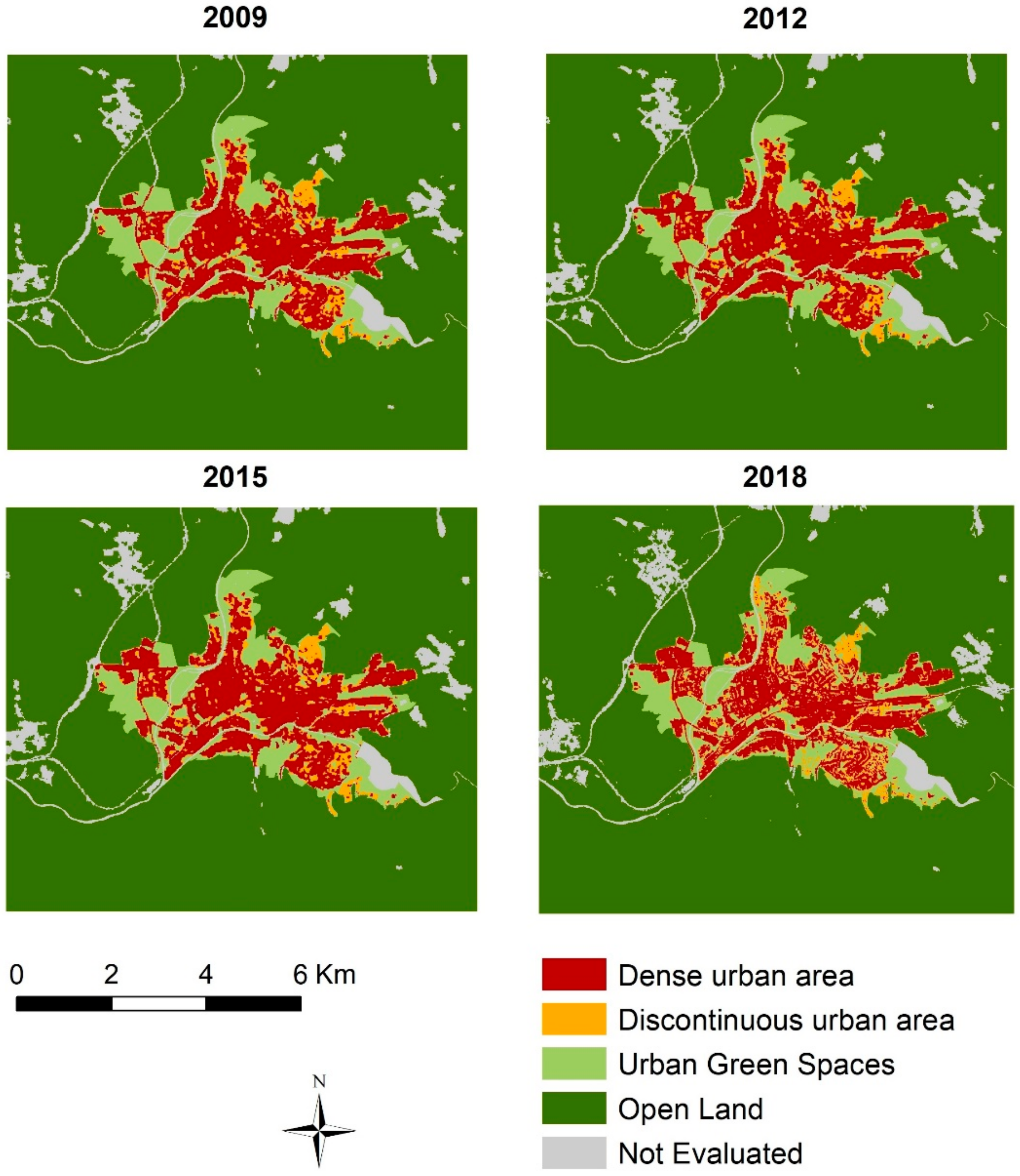
2.5. Spatial Delineation of Urban Zones
2.6. Statistical Analysis
3. Results and Discussion
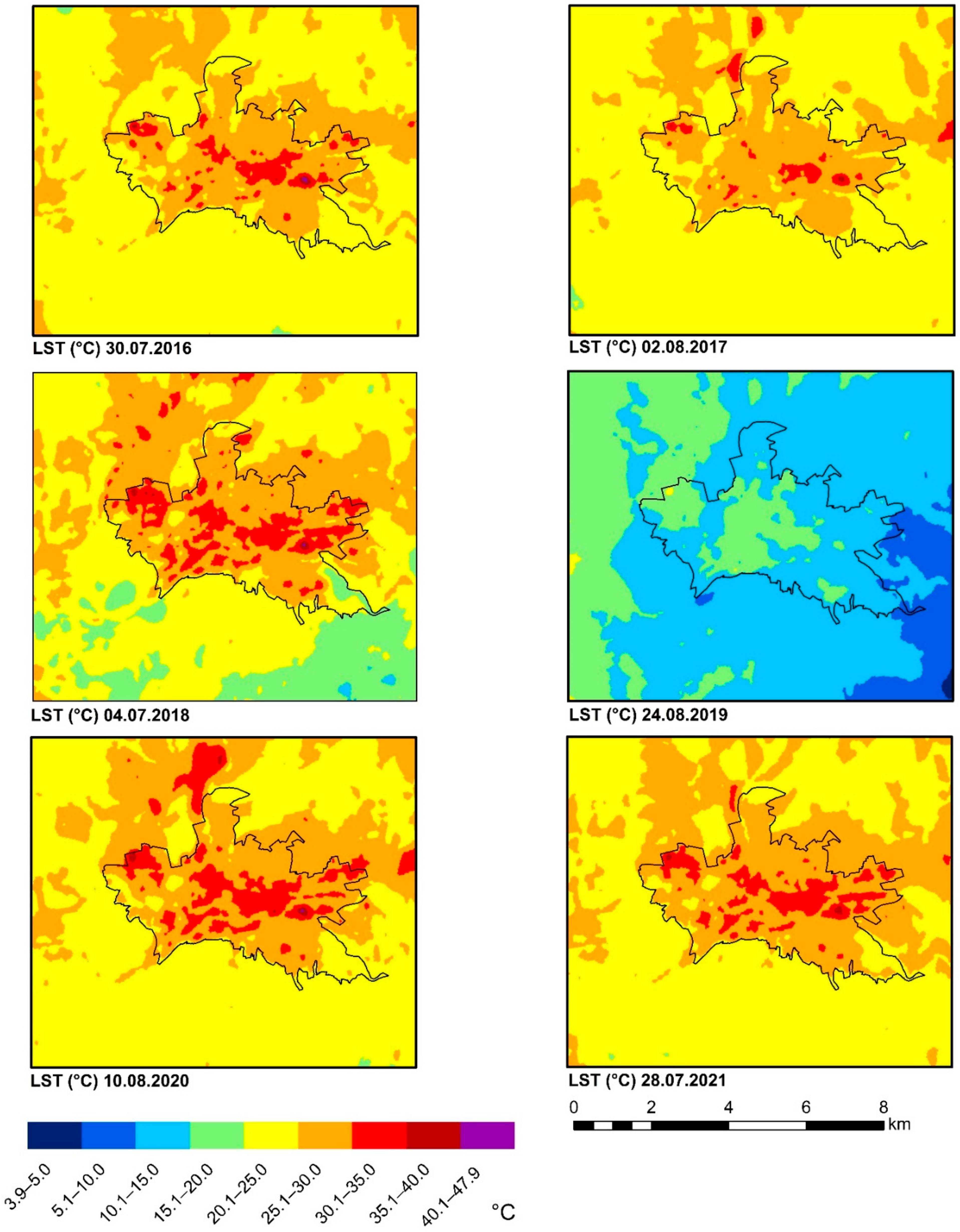
3.1. Analysis of Land Surface Temperature
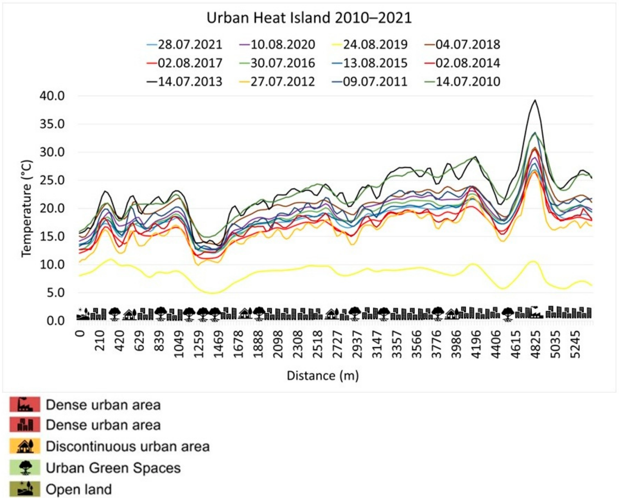
3.2. Evaluation of the Spatial Pattern of Surface Urban Heat Island
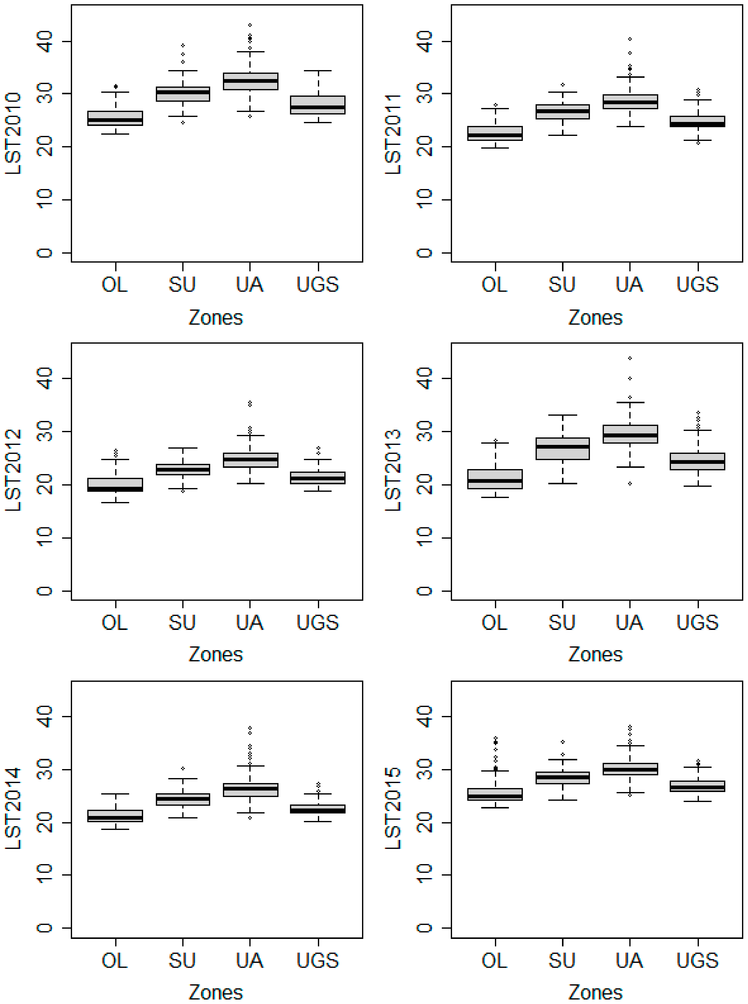
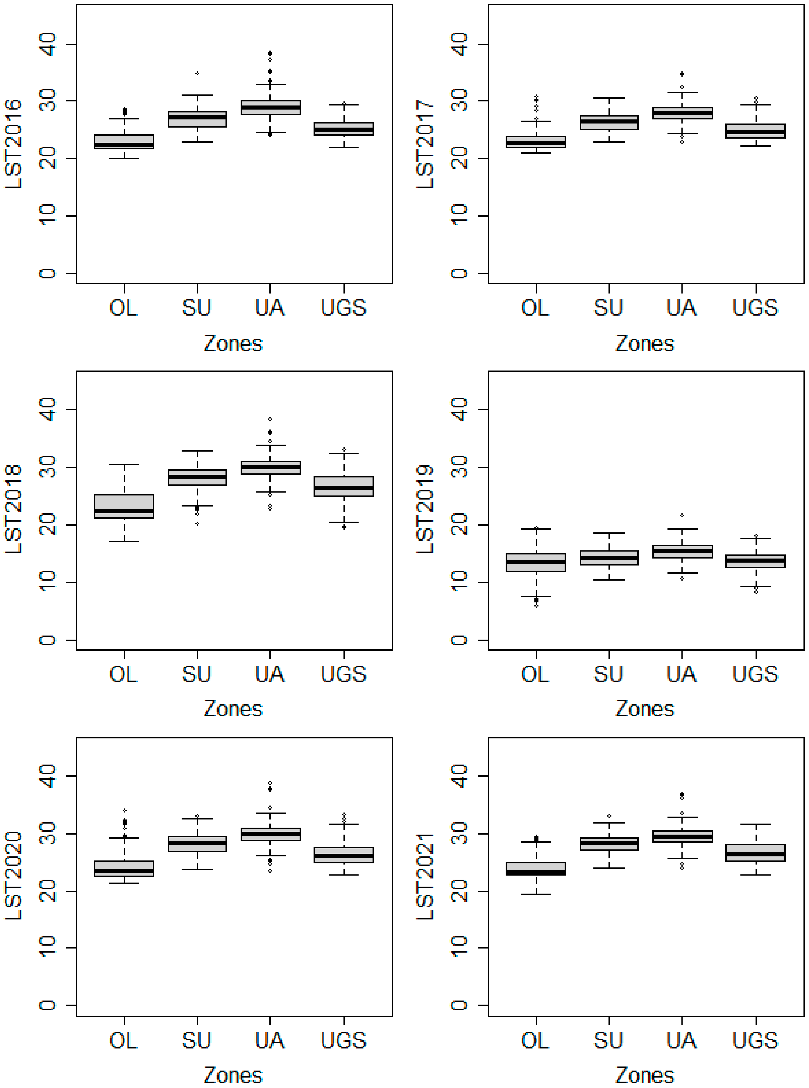
3.3. Comparison of SUHII Differences between Urban Zones with Each Other and between Urban Zones and Open Land
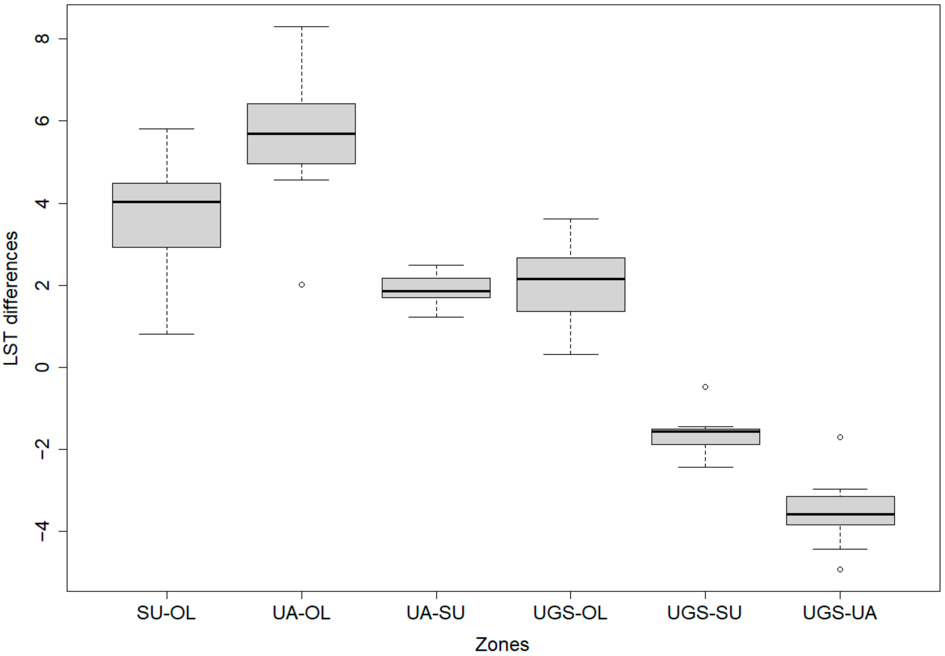
3.4. Evaluation of the Magnitude of SUHII differences between Zones
4. Conclusions
Supplementary Materials
Author Contributions
Funding
Data Availability Statement
Acknowledgments
Conflicts of Interest
References
- Continuing Urbanisation. Available online: https://knowledge4policy.ec.europa.eu/continuing-urbanisation_en (accessed on 10 June 2022).
- Marzluff, J.; Shulenberger, E.; Endlicher, W.; Bradley, G.; Simon, U.; Alberti, M.; Ryan, C.; ZumBrunnen, C. Urban Ecology–An International Perspective on the Interaction between Humans and Nature; Springer: New York, NY, USA, 2008; 807p. [Google Scholar]
- Gartland, L. Heat Islands. Understanding and Mitigating Heat in Urban Areas; Earthscan; Routledge: London, UK, 2008; 215p. [Google Scholar]
- Dadvand, P.; Bartoll, X.; Basagaña, X.; Dalmau-Bueno, A.; Martinez, D.; Ambros, A.; Cirach, M.; Triguero-Mas, M.; Gascon, M.; Borrell, C.; et al. Green spaces and general health: Roles of mental health status, social support, and physical activity. Environ. Int. 2016, 91, 161–167. [Google Scholar] [CrossRef] [PubMed]
- Parris, K. Ecology of Urban Environments; Wiley-Blackwell: Hoboken, NJ, USA, 2016; 240p. [Google Scholar]
- Cui, L.; Shi, J. Urbanization and its environmental effects in Shanghai, China. Urban Clim. 2012, 2, 1–15. [Google Scholar] [CrossRef]
- Kalnay, E.; Cai, M. Impact of urbanization and land-use change on climate. Nature 2003, 423, 528–531. [Google Scholar] [CrossRef] [PubMed]
- Shorabeh, S.N.; Kakroodia, A.A.; Firozjaei, M.K.; Minaeia, F.; Homaee, M. Impact assessment modeling of climatic conditions on spatial-temporal changes in surface biophysical properties driven by urban physical expansion using satellite images. Sustain. Cities Soc. 2022, 80, 103757. [Google Scholar] [CrossRef]
- Voogt, J.A.; Oke, T.R. Thermal remote sensing of urban climates. Remote Sens. Environ. 2003, 86, 370–384. [Google Scholar] [CrossRef]
- Oke, T.R.; Mills, R.; Christen, A.; Voogt, J.A. Urban Climates; Cambridge University Press: Cambridge, UK, 2017; 519p. [Google Scholar] [CrossRef]
- Stewart, I.D.; Mills, G. The Urban Heat Island. A Guidebook, 1st ed.; Elsevier: Amsterdam, the Netherlands, 2021; 182p. [Google Scholar] [CrossRef]
- Butera, F.M. Climatic change and the built environment. Adv. Build. Energy Res. 2010, 4, 45–75. [Google Scholar] [CrossRef]
- Kapsomenakis, J.; Kolokotsa, D.; Nikolaou, T.; Santamouris, M.; Zerefos, S.C. Forty years increase of the air ambient temperature in Greece: The impact on buildings. Energy Convers. Manag. 2013, 74, 353–365. [Google Scholar] [CrossRef]
- Irmak, M.A.; Yilmaz, S.; Dursun, D. Effect of different pavements on human thermal comfort conditions. Atmósfera 2017, 30, 355–366. [Google Scholar] [CrossRef] [Green Version]
- Unger, J. Comparisons of urban and rural bioclimatological conditions in the case of a Central-European city. Int. J. Biometeorol. 1999, 43, 139–144. [Google Scholar] [CrossRef]
- Morris, K.I.; Kwami, A.C.; Kwami Morris, J.; Ooi, M.C.G.; Oozeer, M.Y.; Abakr, Y.A.; Nadzir, M.S.M.; Mohammed, I.Y.; Al-Qrimli, H.F. Impact of urbanization level on the interactions of urban area, the urban climate, and human thermal comfort. Appl. Geogr. 2017, 79, 50–72. [Google Scholar] [CrossRef]
- Givoni, B. Urban design for hot humid regions. Renew. Energy 1994, 5, 1047–1053. [Google Scholar] [CrossRef]
- Lobaccaro, G.; Acero, J.A. Comparative analysis of green actions to improve outdoor thermal comfort inside typical urban street canyons. Urban Clim. 2015, 14, 251–267. [Google Scholar] [CrossRef]
- Yan, H.; Wu, F.; Dong, L. Influence of a large urban park on the local urban thermal environment. Sci. Total Environ. 2018, 622–623, 882–891. [Google Scholar] [CrossRef]
- Teixeira, C.F.B. Green space configuration and its impact on human behavior and urban environments. Urban Clim. 2021, 35, 100746. [Google Scholar] [CrossRef]
- Vieira, J.; Matos, P.; Mexia, T.; Silva, P.; Lopes, N.; Freitas, C.; Correia, O.; Santos-Reis, M.; Branquinho, C.; Pinho, P. Green spaces are not all the same for the provision of air purification and climate regulation services: The case of urban parks. Environ. Res. 2018, 160, 306–313. [Google Scholar] [CrossRef] [PubMed]
- Hondula, D.M.; Davis, R.E.; Leisten, M.J.; Saha, M.V.; Veazey, L.M.; Wegner, C.R. Fine-scale spatial variability of heat-related mortality in Philadelphia County, USA, from 1983–2008: A case-series analysis. Environ. Health A Glob. Access Sci. Source 2012, 11, 16. [Google Scholar] [CrossRef]
- Ingole, V.; Marí-Dell’Olmo, M.; Deluca, A.; Quijal, M.; Borrell, C.; Rodríguez-Sanz, M.; Achebak, H.; Lauwaet, D.; Gilabert, J.; Murage, P.; et al. Spatial Variability of Heat-Related Mortality in Barcelona from 1992–2015: A Case Crossover Study Design. Int. J. Environ. Res. Public Health 2020, 17, 2553. [Google Scholar] [CrossRef]
- Fenner, D.; Holtmann, A.; Meier, F.; Langer, I.; Scherer, D. Contrasting changes of urban heat island intensity during hot weather episodes. Environ. Res. Lett. 2019, 14, 124013. [Google Scholar] [CrossRef]
- Estoque, R.C.; Murayama, Y. Monitoring surface urban heat island formation in a tropical mountain city using Landsat data (1987–2015). ISPRS J. Photogramm. Remote Sens. 2007, 133, 18–29. [Google Scholar] [CrossRef]
- Meehl, G.A.; Tebaldi, C. More intense, more frequent, and longer lasting heat waves in the 21st Century. Science 2004, 305, 994–997. [Google Scholar] [CrossRef]
- Zhou, B.; Rybski, D.; Kropp, J.P. The role of city size and urban form in the surface urban heat island. Sci. Rep. 2017, 7, 4791. [Google Scholar] [CrossRef] [PubMed]
- Leal Filho, W.; Wolf, F.; Castro-Díaz, R.; Li, C.; Ojeh, V.N.; Gutiérrez, N.; Nagy, G.J.; Savić, S.; Natenzon, C.E.; Quasem Al-Amin, A.; et al. Addressing the Urban Heat Islands Effect: A Cross-Country Assessment of the Role of Green Infrastructure. Sustainability 2021, 13, 753. [Google Scholar] [CrossRef]
- Runnalls, K.E.; Oke, T.R. Dynamics and controls of the near-surface heat island of Vancouver, BC. Phys. Geogr. 2000, 21, 283–304. [Google Scholar] [CrossRef]
- Imhoff, M.L.; Yhang, P.; Wolfe, R.E.; Bounoua, L. Remote sensing of the urban heat island effect across biomes in the continental USA. Remote Sens. Environ. 2010, 114, 504–513. [Google Scholar] [CrossRef]
- Hardin, A.W.; Liu, Y.; Cao, G.; Vanos, J.K. Urban heat island intensity and spatial variability by synoptic weather type in the northeast U.S. Urban Clim. 2018, 24, 747–762. [Google Scholar] [CrossRef]
- Kim, S.W.; Brown, R.D. Urban heat island (UHI) intensity and magnitude estimations: A systematic literature review. Sci. Total Environ. 2021, 779, 146389. [Google Scholar] [CrossRef]
- Oke, T.R. City size and the urban heat island. Atmos. Environ. 1973, 7, 769–779. [Google Scholar] [CrossRef]
- Ramakreshnan, L.; Aghamohammadi, N.; Fong, C.S.; Ghaffarianhoseini, A.; Wong, L.P.; Sulaiman, N.M. Empirical study on temporal variations of canopy-level Urban Heat Island effect in the tropical city of Greater Kuala Lumpur. Sustain. Cities Soc. 2019, 44, 748–762. [Google Scholar] [CrossRef]
- Zou, Z.; Yan, C.; Yu, L.; Jiang, X.; Ding, J.; Qin, L.; Wang, B.; Qiu, G. Impacts of land use/land cover types on interactions between urban heat island effects and heat waves. Build. Environ. 2021, 204, 108138. [Google Scholar] [CrossRef]
- Rajkovich, N.B.; Larsen, L. A Bicycle-Based Field Measurement System for the Study of Thermal Exposure in Cuyahoga County, Ohio, USA. Int. J. Environ. Res. Public Health 2016, 13, 159. [Google Scholar] [CrossRef]
- Schwarz, N.; Lautenbach, S.; Seppelt, R. Exploring indicators for quantifying surface urban heat islands of European cities with MODIS land surface temperatures. Remote Sens. Environ. 2011, 115, 3175–3186. [Google Scholar] [CrossRef]
- Zhou, D.; Zhao, S.; Liu, S.; Zhang, L.; Zhu, C. Surface urban heat island in China’s 32 major cities: Spatial patterns and drivers. Remote Sens. Environ. 2014, 152, 51–61. [Google Scholar] [CrossRef]
- Liu, K.; Su, H.; Zhang, L.; Yang, H.; Zhang, R.; Li, X. Analysis of the Urban Heat Island Effect in Shijiazhuang, China Using Satellite and Airborne Data. Remote Sens. 2015, 7, 4804–4833. [Google Scholar] [CrossRef]
- Almeida, C.R.d.; Teodoro, A.C.; Gonçalves, A. Study of the Urban Heat Island (UHI) Using Remote Sensing Data/Techniques: A Systematic Review. Environments 2021, 8, 105. [Google Scholar] [CrossRef]
- Marando, F.; Salvatori, E.; Sebastiani, A.; Fusaro, L.; Manes, F. Regulating Ecosystem Services and Green Infrastructure: Assessment of Urban Heat Island effect mitigation in the municipality of Rome, Italy. Ecol. Model. 2019, 392, 92–102. [Google Scholar] [CrossRef]
- EPA (US Environmental Protection Agency). Reducing Urban Heat Islands: Compendium of Strategies; US Environmental Protection Agency: Washington, DC, USA, 2008; 19p.
- Kim, S.W.; Brown, R.D. Urban heat island (UHI) variations within a city boundary: A systematic literature review. Renew. Sustain. Energy Rev. 2021, 148, 111256. [Google Scholar] [CrossRef]
- Xu, L.Y.; Xie, X.D.; Li, S. Correlation analysis of the urban heat island effect and the spatial and temporal distribution of atmospheric particulates using TM images in Beijing. Environ. Pollut. 2013, 178, 102–114. [Google Scholar] [CrossRef] [PubMed]
- Arnfield, A.J. Two decades of urban climate research: A review of turbulence, exchanges of energy and water, and the urban heat island. Int. J. Clim. 2003, 23, 1–26. [Google Scholar] [CrossRef]
- Zhou, W.; Huang, G.; Cadenasso, M.L. Does spatial configuration matter? Understanding the effects of land cover pattern on land surface temperature in urban landscapes. Landsc. Urban Plan. 2011, 102, 54–63. [Google Scholar] [CrossRef]
- Tzavali, A.; Paravantis, J.; Mihalakakou, G.; Fotiadi, A.; Stigka, E. Urban heat island intensity: A literature review. Fresenius Environ. Bull. 2015, 24, 4537–4554. [Google Scholar]
- Li, Y.; Zhang, X.; Zhu, S.; Wang, X.; Lu, Y.; Du, S.; Shi, X. Transformation of Urban Surfaces and Heat Islands in Nanjing during 1984–2018. Sustainability 2020, 12, 6521. [Google Scholar] [CrossRef]
- Keeratikasikorn, C.; Bonafoni, S. Urban Heat Island Analysis over the Land Use Zoning Plan of Bangkok by Means of Landsat 8 Imagery. Remote Sens. 2018, 10, 440. [Google Scholar] [CrossRef]
- Yu, Z.; Yao, Y.; Yang, G.; Wang, X.; Vejre, H. Spatiotemporal patterns and characteristics of remotely sensed region heat islands during the rapid urbanization (1995–2015) of Southern China. Sci. Total Environ. 2019, 674, 242–254. [Google Scholar] [CrossRef]
- Sun, Y.; Gao, C.; Li, J.; Wang, R.; Liu, J. Evaluating urban heat island intensity and its associated determinants of towns and cities continuum in the Yangtze River Delta Urban Agglomerations. Sustain. Cities Soc. 2019, 50, 101659. [Google Scholar] [CrossRef]
- Zhang, X.; Chen, L.; Jianf, W.; Jin, X. Urban heat island of Yangtze River Delta urban agglomeration in China: Multi-time scale characteristics and influencing factors. Urban Clim. 2022, 43, 101180. [Google Scholar] [CrossRef]
- Busato, F.; Lazzarin, R.M.; Noro, M. Three years of study of the Urban Heat Island in Padua: Experimental results. Sustain. Cities Soc. 2014, 10, 251–258. [Google Scholar] [CrossRef]
- Blachowski, J.; Hajnrych, M. Assessing the Cooling Effect of Four Urban Parks of Different Sizes in a Temperate Continental Climate Zone: Wroclaw (Poland). Forests 2021, 12, 1136. [Google Scholar] [CrossRef]
- Song, J.; Du, S.; Feng, X.; Guo, L. The relationships between landscape compositions and land surface temperature: Quantifying their resolution sensitivity with spatial regression models. Landsc. Urban Plan. 2014, 123, 145–157. [Google Scholar] [CrossRef]
- Bokaie, M.; Shamsipour, A.; Khatibi, P.; Hosseini, A. Seasonal monitoring of urban heat island using multi-temporal Landsat and MODIS images in Tehran. Int. J. Urban Sci. 2019, 23, 269–285. [Google Scholar] [CrossRef]
- Amir Siddique, M.; Wang, Y.; Xu, N.; Ullah, N.; Zeng, P. The Spatiotemporal Implications of Urbanization for Urban Heat Islands in Beijing: A Predictive Approach Based on CA–Markov Modeling (2004–2050). Remote Sens. 2021, 13, 4697. [Google Scholar] [CrossRef]
- Peng, J.; Liu, Q.; Xu, Z.; Lyu, D.; Du, Y.; Qiao, P.; Wu, J. How to effectively mitigate urban heat island effect? A perspective of waterbody patch size threshold. Landsc. Urban Plan. 2020, 202, 103873. [Google Scholar] [CrossRef]
- Athukorala, D.; Murayama, Y. 2021: Urban Heat Island Formation in Greater Cairo: Spatio-Temporal Analysis of Daytime and Nighttime Land Surface Temperatures along the Urban–Rural Gradient. Remote Sens. 2021, 13, 1396. [Google Scholar] [CrossRef]
- Li, X.; Zhou, W.; Ouyang, Z.; Xu, W.; Zheng, H. Spatial pattern of greenspace affects land surface temperature: Evidence from the heavily urbanized Beijing metropolitan area, China. Landsc. Ecol. 2012, 27, 887–898. [Google Scholar] [CrossRef]
- Onishi, A.; Cao, X.; Ito, T.; Shi, F.; Imura, H. Evaluating the potential for urban heat-island mitigation by greening parking lots. Urban For. Urban Green. 2010, 9, 323–332. [Google Scholar] [CrossRef]
- Zhang, Y.; Balzter, H.; Li, Y. Influence of Impervious Surface Area and Fractional Vegetation Cover on Seasonal Urban Surface Heating/Cooling Rates. Remote Sens. 2021, 13, 1263. [Google Scholar] [CrossRef]
- O’Malley, C.; Piroozfar, P.; Farr, E.R.P.; Pomponi, F. Urban Heat Island (UHI) mitigating strategies: A case-based comparative analysis. Sustain. Cities Soc. 2015, 19, 222–235. [Google Scholar] [CrossRef]
- Grilo, F.; Pinho, P.; Aleixo, C.; Catita, C.; Silva, P.; Lopes, N.; Freitas, C.; Santos-Reis, M.; McPhearson, T.; Branquinho, C. Using green to cool the grey: Modelling the cooling effect of green spaces with a high spatial resolution. Sci. Total Environ. 2020, 724, 138182. [Google Scholar] [CrossRef]
- Dimoudi, A.; Nikolopoulou, M. Vegetation in the urban environment: Microclimatic analysis and benefits. Energy Build. 2003, 35, 69–76. [Google Scholar] [CrossRef]
- Pauleit, S.; Hansen, R.; Rall, E.L.; Zölch, T.; Andersson, E.; Luz, A.C.; Szaraz, L.; Tosics, I.; Vierikko, K. Urban Landscapes and Green Infrastructure; Oxford University Press: Oxford, UK, 2017; 53p. [Google Scholar] [CrossRef]
- Aram, F.; Garcia, E.H.; Solgi, E.; Mansournia, S. Urban green space cooling effect in cities. Review Article. Heliyon 2019, 5, e01339. [Google Scholar] [CrossRef]
- Feyisa, G.L.; Dons, K.; Meilby, H. Efficiency of parks in mitigating urban heat island effect: An example from Addis Ababa. Landsc. Urban Plan. 2014, 123, 87–95. [Google Scholar] [CrossRef]
- Shashua-Bar, L.; Pearlmutter, D.; Erell, E. The cooling efficiency of urban landscape strategies in a hot dry climate. Landsc. Urban Plan. 2009, 92, 179–186. [Google Scholar] [CrossRef]
- Cao, X.; Onishi, A.; Chen, J.; Imura, H. Quantifying the cool island intensity of urban parks using ASTER and IKONOS data. Landsc. Urban Plan. 2010, 96, 224–231. [Google Scholar] [CrossRef]
- Derkzen, M.L.; van Teeffelen, A.J.A.; Verburg, P.H. Quantifying urban ecosystem services based on highresolution data of urban green space: An assessment for Rotterdam, the Netherlands. J. Appl. Ecol. 2015, 52, 1020–1032. [Google Scholar] [CrossRef]
- Pinho, P.; Correia, O.; Lecoq, M.; Munzi, S.; Vasconcelos, S.; Gonçalves, P.; Rebelo, R.; Antunes, C.; Silva, P.; Freitas, C.; et al. Evaluating green infrastructure in urban environments using a multi-taxa and functional diversity approach. Environ. Res. 2016, 147, 601–610. [Google Scholar] [CrossRef]
- Villalobos-Jiménez, G.; Dunn, A.; Hassall, C. Dragonflies and damselflies (Odonata) in urban ecosystems: A review. Eur. J. Entomol. 2016, 113, 217–232. [Google Scholar] [CrossRef]
- Langemeyer, J. Urban Ecosystem Services. The Value of Green Spaces in Cities; Stockholm University: Stockholm, Sweden, 2015; 246p. [Google Scholar]
- Mexia, T.; Vieira, J.; Príncipe, A.; Anjos, A.; Silva, P.; Lopes, N.; Freitas, C.; Santos-Reis, M.; Correia, O.; Branquinho, C.; et al. Ecosystem services: Urban parks under a magnifying glass. Environ. Res. 2018, 160, 469–478. [Google Scholar] [CrossRef]
- Costanza, R.; D’Arge, R.; de Groot, R.S.; Farber, S.; Grasso, M.; Hannon, B.; Limburg, K.; Naeem, S.; O’Neill, R.V.; Paruelo, J.; et al. The value of world’s ecosystem services and natural capital. Nature 1997, 387, 253–260. [Google Scholar] [CrossRef]
- Daily, G.C. (Ed.) Nature’s Services Societal Dependence On Natural Ecosystems; Island Press: Washington, DC, USA, 1997; 392p. [Google Scholar]
- Millennium Ecosystem Assessment. Ecosystems and Human Well-Being–Synthesis; Island Press: Washington, DC, USA, 2005; Available online: https://millenniumassessment.org/en/index.html (accessed on 20 June 2022).
- Park, J.; Kim, J.-H.; Lee, D.K.; Park, C.Y.; Jeong, S.G. The influence of small green space type and structure at the street level on urban heat island mitigation. Urban For. Urban Green. 2017, 21, 203–212. [Google Scholar] [CrossRef]
- Rakoto, P.Y.; Deilami, K.; Hurley, J.; Amati, M.; Sun, Q.C. Revisiting the cooling effects of urban greening: Planning implications of vegetation types and spatial configuration. Urban For. Urban Green. 2021, 64, 127266. [Google Scholar] [CrossRef]
- Zhou, W.; Cao, F.; Wang, G. Effects of Spatial Pattern of Forest Vegetation on Urban Cooling in a Compact Megacity. Forests 2019, 10, 282. [Google Scholar] [CrossRef]
- Su, Y.; Wu, J.; Zhang, C.; Wu, X.; Li, Q.; Bi, C.; Zhang, H.; Lafortezza, R.; Chen, X. Estimating the cooling effect magnitude of urban vegetation in different climate zones using multi-source remote sensing. Urban Clim. 2022, 43, 101155. [Google Scholar] [CrossRef]
- World Health Organization; Regional Office for Europe. Health and Climate Change: The “Now and How”: A Policy Action Guide; World Health Organization; Regional Office for Europe: Geneva, Switzerland, 2005; 32p. Available online: https://apps.who.int/iris/handle/10665/347913 (accessed on 20 June 2022).
- ZBGIS® 2021. Basic Database for the Geographic Information System. Geodetic and Cartographic Institute Bratislava (GKÚ) Slovakia. Available online: https://zbgis.skgeodesy.sk/mkzbgis/sk/zakladna-mapa?pos=48.800000,19.530000,8 (accessed on 5 April 2022).
- Corine Land Cover 2018. Copernicus Land Monitoring Service. Available online: https://land.copernicus.eu/pan-european/corine-land-cover/clc2018?tab=download (accessed on 5 April 2022).
- Derdouri, A.; Wang, R.; Murayama, Y.; Osaragi, T. Understanding the Links between LULC Changes and SUHI in Cities: Insights from Two-Decadal Studies (2001–2020). Remote Sens. 2021, 13, 3654. [Google Scholar] [CrossRef]
- Klok, L.; Zwart, S.; Verhagen, H.; Mauri, E. The surface heat island of Rotterdam and its relationship with urban surface characteristics. Resour. Conserv. Recycl. 2012, 64, 23–29. [Google Scholar] [CrossRef]
- United States Geological Survey (USGS) EarthExplorer. Available online: https://earthexplorer.usgs.gov/ (accessed on 6 April 2022).
- Landsat Satellite Missions. United States Geological Survey. Available online: https://www.usgs.gov/landsat-missions/landsat-satellite-missions (accessed on 6 April 2022).
- Orthophotomosaic. Geodetic and Cartographic Institute Bratislava (GKÚ) Slovakia, National Forest Centre (NLC) Slovakia. Available online: https://www.geoportal.sk (accessed on 5 April 2022).
- Imperviousness Density, Copernicus Land Monitoring Service. Available online: https://land.copernicus.eu/pan-european/high-resolution-layers/imperviousness/status-maps (accessed on 6 April 2022).
- ESRI®. Available online: https://www.esri.com (accessed on 4 April 2022).
- R Core Team. R: A Language and Environment for Statistical Computing; R Foundation for Statistical Computing: Vienna, Austria, 2020; Available online: https://www.R-project.org/ (accessed on 5 May 2022).
- Chander, G.; Markham, B. Revised Landsat-5 TM Radiometric Calibration Procedures and Postcalibration Dynamic Ranges. IEEE Trans. Geosci. Remote Sens. 2003, 41, 2674–2677. [Google Scholar] [CrossRef]
- Yuan, F.; Bauer, M.E. Comparison of impervious surface area and normalized difference vegetation index as indicators of surface urban heat island effects in Landsat imagery. Remote Sens. Environ. 2007, 106, 375–386. [Google Scholar] [CrossRef]
- Carlson, T.N.; Ripley, D.A. On the relation between NDVI, fractional vegetation cover, and leaf area index. Remote Sens. Environ. 1997, 62, 241–252. [Google Scholar] [CrossRef]
- Sobrino, J.A.; Jiménez-Muñoz, J.C.; Paolini, L. 2004: Land surface temperature retrieval from LANDSAT TM 5. Remote Sens. Environ. 2004, 90, 434–440. [Google Scholar] [CrossRef]
- Barsi, J.A.; Schott, J.R.; Palluconi, F.D.; Hook, S.J. Validation of a web-based atmospheric correction tool for single thermal band instruments. Proc. SPIE 2005, 5882, 58820E. [Google Scholar]
- Lepš, J.; Šmilauer, P. Biostatistics with R: An Introductory Guide for Field Biologists, 1st ed.; Cambridge University Press: Cambridge, UK, 2020; 382p. [Google Scholar]
- Zar, J.H. Biostatistical Analysis, 5th ed.; Prentice-Hall/Pearson: Upper Saddle River, NJ, USA, 2010; 944p. [Google Scholar]
- Logan, M. Biostatistical Design and Analysis Using, R. A Practical Guide; Wiley-Blackwell: Hoboken, NJ, USA, 2010; 546p. [Google Scholar]
- Le, C.T.; Eberly, L.E. Introductory Biostatistics, 2nd ed.; Wiley: Hoboken, NJ, USA, 2016; 592p. [Google Scholar]
- Yanev, I.; Lachezar, F. Assessment of the land surface temperature dynamics in the city of Sofia using Landsat satellite data. Aerosp. Res. Bulg. 2017, 27, 45–71. [Google Scholar] [CrossRef]
- Jain, S.; Sannigrahi, S.; Sen, S.; Bhatt, S.; Chakraborti, S.; Rahmat, S. Urban heat island intensity and its mitigation strategies in the fastgrowing urban area. J. Urban Manag. 2020, 9, 54–66. [Google Scholar] [CrossRef]
- Ma, Y.; Kuang, Y.; Huang, N. Coupling urbanization analyses for studying urban thermal environment and its interplay with biophysical parameters based on TM/ETM+ imagery. Int. J. Appl. Earth Obs. Geoinf. 2010, 12, 110–118. [Google Scholar] [CrossRef]
- Li, H.; Zhou, Y.; Li, X.; Meng, L.; Wang, X.; Wu, S.; Sodoudi, S. A new method to quantify surface urban heat island intensity. Sci. Total Environ. 2008, 624, 262–272. [Google Scholar] [CrossRef] [PubMed]
- Zhu, W.; Sun, J.; Yang, C.; Liu, M.; Xu, X.; Ji, C. How to Measure the Urban Park Cooling Island? A Perspective of Absolute and Relative Indicators Using Remote Sensing and Buffer Analysis. Remote Sens. 2021, 13, 3154. [Google Scholar] [CrossRef]
- Yan, L.; Jia, W.; Zhao, S. The Cooling Effect of Urban Green Spaces in Metacities: A Case Study of Beijing, China’s Capital. Remote Sens. 2021, 13, 4601. [Google Scholar] [CrossRef]
- Coutts, A.M.; Harris, R.J.; Phan, T.; Livesley, S.J.; Williams, N.S.G.; Tapper, N.J. Thermal infrared remote sensing of urban heat: Hotspots, vegetation, and an assessment of techniques for use in urban planning. Remote Sens. Environ. 2016, 186, 637–651. [Google Scholar] [CrossRef]
- Rogan, J.; Ziemer, M.; Martin, D.; Ratick, S.; Cuba, N.; DeLauer, V. The impact of tree cover loss on land surface temperature: A case study of central Massachusetts using Landsat Thematic Mapper thermal data. Appl. Geogr. 2013, 45, 49–57. [Google Scholar] [CrossRef]
- Lin, W.; Yu, T.; Chang, X.; Wu, W.; Zhang, Y. Calculating cooling extents of green parks using remote sensing: Method and test. Landsc. Urban Plan. 2015, 134, 66–75. [Google Scholar] [CrossRef]
- Du, J.; Xiang, X.; Zhao, B.; Zhou, H. Impact of urban expansion on land surface temperature in Fuzhou, China using Landsat imagery. Sustain. Cities Soc. 2020, 61, 102346. [Google Scholar] [CrossRef]
- Lepeška, T. The impact of impervious surfaces on ecohydrology and health in urban ecosystems of Banská Bystrica (Slovakia). Soil Water Res. 2016, 11, 29–36. [Google Scholar] [CrossRef] [Green Version]
- Izakovičová, Z.; Mederly, P.; Petrovič, F. Long-Term Land Use Changes Driven by Urbanisation and Their Environmental Effects (Example of Trnava City, Slovakia). Sustainability 2017, 9, 1553. [Google Scholar] [CrossRef]
- Hellings, A.; Rienow, A. Mapping Land Surface Temperature Developments in Functional Urban Areas across Europe. Remote Sens. 2021, 13, 2111. [Google Scholar] [CrossRef]
- Wang, H.; Li, B.; Yi, T.; Wu, J. Heterogeneous Urban Thermal Contribution of Functional Construction Land Zones: A Case Study in Shenzhen, China. Remote Sens. 2022, 14, 1851. [Google Scholar] [CrossRef]
- Yu, X.; Guo, X.; Wu, Z. Land Surface Temperature Retrieval from Landsat 8 TIRS—Comparison between Radiative Transfer Equation-Based Method, Split Window Algorithm and Single Channel Method. Remote Sens. 2014, 6, 9829–9852. [Google Scholar] [CrossRef]
- García-Santos, V.; Cuxart, J.; Martínez-Villagrasa, D.; Jiménez, M.A.; Simó, G. Comparison of Three Methods for Estimating Land Surface Temperature from Landsat 8-TIRS Sensor Data. Remote Sens. 2018, 10, 1450. [Google Scholar] [CrossRef]
- Jiang, Y.; Lin, W. A Comparative Analysis of Retrieval Algorithms of Land Surface Temperature from Landsat-8 Data: A Case Study of Shanghai, China. Int. J. Environ. Res. Public Health 2021, 18, 5659. [Google Scholar] [CrossRef]
- Li, F.; Jackson, T.J.; Kustas, W.P.; Schmugge, T.J.; French, A.N.; Cosh, M.H.; Bindlish, R. Deriving land surface temperature from Landsat 5 and 7 during SMEX02/SMACEX. Remote Sens. Environ. 2004, 92, 521–534. [Google Scholar] [CrossRef]
- Simó, G.; García-Santos, V.; Jiménez, M.A.; Martínez-Villagrasa, D.; Picos, R.; Caselles, V.; Cuxart, J. Landsat and Local Land Surface Temperatures in a Heterogeneous Terrain Compared to MODIS Values. Remote Sens. 2016, 8, 849. [Google Scholar] [CrossRef]
- Laraby, K.G.; Schott, J.R. Uncertainty estimation method and Landsat 7 global validation for the Landsat surface temperature product. Remote Sens. Environ. 2018, 216, 472–481. [Google Scholar] [CrossRef]
- Yu, K.; Chen, Y.; Wang, D.; Chen, Z.; Gong, A.; Li, J. Study of the Seasonal Effect of Building Shadows on Urban Land Surface Temperatures Based on Remote Sensing Data. Remote Sens. 2019, 11, 497. [Google Scholar] [CrossRef] [Green Version]
- Zhao, W.; Duan, S.-B. Reconstruction of daytime land surface temperatures under cloud-covered conditions using integrated MODIS/Terra land products and MSG geostationary satellite data. Remote Sens. Environ. 2020, 247, 111931. [Google Scholar] [CrossRef]
- Wu, P.; Su, Y.; Duan, S.-B.; Li, X.; Yang, H.; Zeng, C.; Ma, X.; Wu, Y.; Shen, H. A two-step deep learning framework for mapping gapless all-weather land surface temperature using thermal infrared and passive microwave data. Remote Sens. Environ. 2020, 277, 113070. [Google Scholar] [CrossRef]


| Date of Accusations | Satellite | Band Used | Sensor | Resolution | Time (GMT) | Local Time (GMT+1) |
|---|---|---|---|---|---|---|
| 14.07.2010 | Landsat-5 | Band 6 | TM/TIRS | 30/120 | 09:23 | 10:23 |
| 09.07.2011 | Landsat-7 | Band 6 | ETM+ | 30/60 | 09:26 | 10:26 |
| 27.07.2012 | Landsat-7 | Band 6 | ETM+ | 30/60 | 09:27 | 10:27 |
| 14.07.2013 | Landsat-7 | Band 6 | ETM+ | 30/60 | 09:28 | 10:28 |
| 02.08.2014 | Landsat-7 | Band 6 | ETM+ | 30/60 | 09:30 | 10:30 |
| 13.08.2015 | Landsat-8 | Band 10 | OLI/TIRS | 30/100 | 09:32 | 10:32 |
| 30.07.2016 | Landsat-8 | Band 10 | OLI/TIRS | 30/100 | 09:32 | 10:32 |
| 02.08.2017 | Landsat-8 | Band 10 | OLI/TIRS | 30/100 | 09:32 | 10:32 |
| 04.07.2018 | Landsat-8 | Band 10 | OLI/TIRS | 30/100 | 09:31 | 10:31 |
| 24.08.2019 | Landsat-8 | Band 10 | OLI/TIRS | 30/100 | 09:33 | 10:33 |
| 10.08.2020 | Landsat-8 | Band 10 | OLI/TIRS | 30/100 | 09:32 | 10:32 |
| 28.07.2021 | Landsat-8 | Band 10 | OLI/TIRS | 30/100 | 09:32 | 10:32 |
| Band | K1 | K2 | |
|---|---|---|---|
| Landsat-8 OLI/TIRS | Band 10 | 774.8853 | 1321.0789 |
| Landsat-7 ETM+ | Band 6 | 666.09 | 1282.71 |
| Landsat-5 TM | Band 6 | 607.76 | 1260.56 |
| SUHI Intensity Levels | |
|---|---|
| <0 | No SUHII (Green Island) |
| 0–0.1 | Weak heat island |
| 0.1–0.2 | Medium heat island |
| 0.2–0.4 | Strong heat island |
| >0.4 | Extremely strong heat island |
| Date | F (3, 1196) | p (ANOVA) | Difference between Zones (p-Value of Post-Hoc) | |||||
|---|---|---|---|---|---|---|---|---|
| SU–OL | UA–OL | UGS–OL | UA–SU | UGS–SU | UGS–UA | |||
| 14 July 2010 | 616.1 | <0.001 | <0.001 | <0.001 | <0.001 | <0.001 | <0.001 | <0.001 |
| 9 July 2011 | 577.6 | <0.001 | <0.001 | <0.001 | <0.001 | <0.001 | <0.001 | <0.001 |
| 27 July 2012 | 440.1 | <0.001 | <0.001 | <0.001 | <0.001 | <0.001 | <0.001 | <0.001 |
| 14 July 2013 | 595.8 | <0.001 | <0.001 | <0.001 | <0.001 | <0.001 | <0.001 | <0.001 |
| 2 August 2014 | 537.2 | <0.001 | <0.001 | <0.001 | <0.001 | <0.001 | <0.001 | <0.001 |
| 13 August 2015 | 409.2 | <0.001 | <0.001 | <0.001 | <0.001 | <0.001 | <0.001 | <0.001 |
| 30 July 2016 | 654.9 | <0.001 | <0.001 | <0.001 | <0.001 | <0.001 | <0.001 | <0.001 |
| 2 August 2017 | 505.2 | <0.001 | <0.001 | <0.001 | <0.001 | <0.001 | <0.001 | <0.001 |
| 4 July 2018 | 476.9 | <0.001 | <0.001 | <0.001 | <0.001 | <0.001 | <0.001 | <0.001 |
| 24 August 2019 | 72.8 | <0.001 | <0.001 | <0.001 | 0.145 | <0.001 | 0.006 | <0.001 |
| 10 August 2020 | 474.4 | <0.001 | <0.001 | <0.001 | <0.001 | <0.001 | <0.001 | <0.001 |
| 28 July 2021 | 555.6 | <0.001 | <0.001 | <0.001 | <0.001 | <0.001 | <0.001 | <0.001 |
Publisher’s Note: MDPI stays neutral with regard to jurisdictional claims in published maps and institutional affiliations. |
© 2022 by the authors. Licensee MDPI, Basel, Switzerland. This article is an open access article distributed under the terms and conditions of the Creative Commons Attribution (CC BY) license (https://creativecommons.org/licenses/by/4.0/).
Share and Cite
Murtinová, V.; Gallay, I.; Olah, B. Mitigating Effect of Urban Green Spaces on Surface Urban Heat Island during Summer Period on an Example of a Medium Size Town of Zvolen, Slovakia. Remote Sens. 2022, 14, 4492. https://doi.org/10.3390/rs14184492
Murtinová V, Gallay I, Olah B. Mitigating Effect of Urban Green Spaces on Surface Urban Heat Island during Summer Period on an Example of a Medium Size Town of Zvolen, Slovakia. Remote Sensing. 2022; 14(18):4492. https://doi.org/10.3390/rs14184492
Chicago/Turabian StyleMurtinová, Veronika, Igor Gallay, and Branislav Olah. 2022. "Mitigating Effect of Urban Green Spaces on Surface Urban Heat Island during Summer Period on an Example of a Medium Size Town of Zvolen, Slovakia" Remote Sensing 14, no. 18: 4492. https://doi.org/10.3390/rs14184492