A Wideband Noise Radar System Using a Phased Array with True Time Delay

Abstract

Noise radar has become attractive owing to progress in hardware technology. Aside from the low probability of exploitation, the use of noise waveform is likely to grow due to its low interference features, especially in circumstances where multiple radars operate in the same band. In this study, we developed and tested a wideband noise radar for a ground-moving vehicle. It operates in the X-band with an instantaneous bandwidth of 1.5 GHz. The true time delay (TTD) was applied to correct the distortion of the beam pattern by the wide bandwidth, and the correlators were implemented by high-speed parallel processing using a field programmable gate array (FPGA). The outdoor experimental results were presented.

1. Introduction

Noise radar, also known as random noise radar (RNR), was first considered a method for removing both range-Doppler ambiguities in the early 1950s [1]. However, owing to the complexity and a large amount of computation, it was not easy to implement it in actual hardware. Recently, it has been actively studied again and implemented into systems as the hardware, including radio frequency (RF) technology and analog to digital converter (ADC)/digital to analog converter (DAC), has progressed [2,3].

Noise radar detects a target using a low-power continuous signal that appears to be random noise. The key advantage of a noise signal is its low probability of exploitation (LPE) property against electronic support measures (ESM) and electronic intelligence (ELINT). ESM and ELINT are technologies used for detecting, analyzing, and cataloging radar signals. Because of its low power and randomness, noise radar has the advantage of a low probability of detection (LPD). It has a more significant advantage in that the random signal is difficult to catalog and duplicate for deceptive, false target signals [4]. In addition, the ideal noise waveform has no mutual interference; therefore, it can be used in radars operating simultaneously in the same frequency band. For example, as the use of automotive radars is gradually increasing, waveforms of low mutual interference are required, and the noise signal can be a candidate. Furthermore, the low-interference property is critical for a multi-input multi-output (MIMO) radar, which transmits multiple waveforms simultaneously [1]. The final advantage is that there is no ambiguity in range-Doppler measurements with a thumbtack ambiguity function, which is an original characteristic of noise radar. In addition, it has high resolution because the signal is homogeneously spread in frequency and infinitely lasting over time. In practice, the resolution is limited by both the bandwidth and integration time.

However, noise radar has several drawbacks. First, because the transmitting and receiving antennas are separated to employ a low-power continuous wave, their isolation and co-linearity must be satisfactory. Second, depending on the maximum detection range, a wide receiver dynamic range of at least 90 dB is often required. Finally, it requires a huge amount of computational power for the correlators to cover all required ranges and Doppler bins.

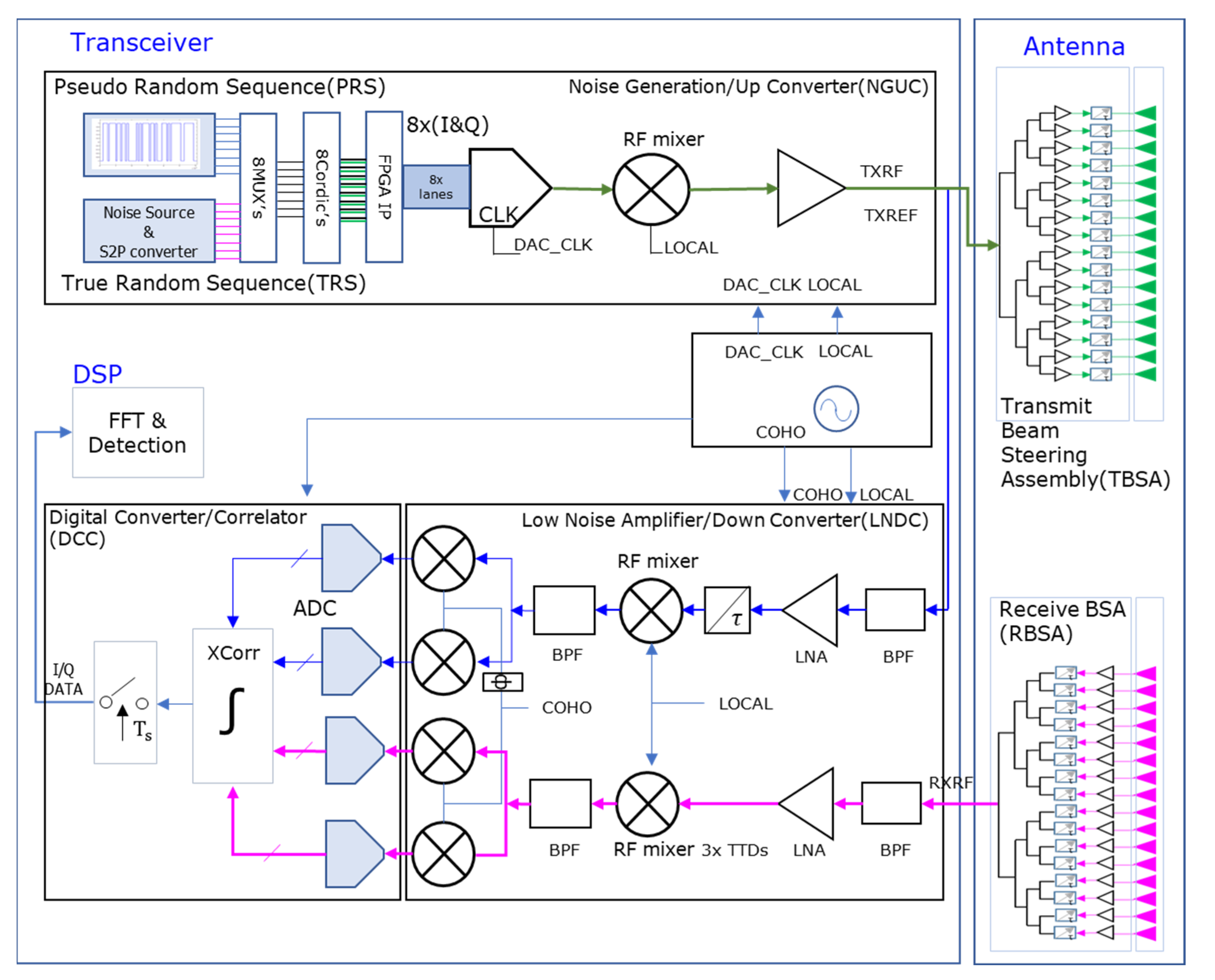
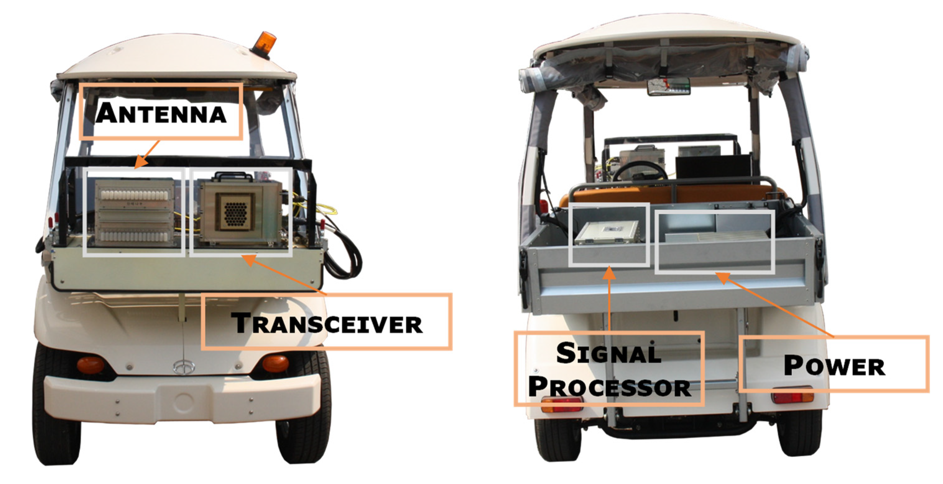
In this study, we developed and tested a wideband noise radar that operates in a ground-moving vehicle. It operates in the X-band, with an instantaneous bandwidth of 1.5 GHz. The antenna is made up of linear arrays. The receiver was built using high-speed digital electronics, including ADCs and FPGAs. This system has a wide bandwidth of up to 15% of the center frequency and a beamformer that uses a true time delay (TTD) to prevent pattern distortion in the array antenna using phase shifters. Furthermore, by employing the time-division method, the FPGA’s computational resources for implementing correlators are reduced to a quarter.

TTD employs the time delay of the actual path difference. Consequently, unlike the phase shifter, it preserves the beam pattern even when the signal has a wide bandwidth [5,6,7,8,9]. However, because the physical size is large, the maximum delay time is bounded, and the implementation of a large number of arrays is limited. Sub-array network structure in parallel with phase shifters was introduced to reduce the number of TTDs [10]. If all array signals are converted to digital data, the analog TTDs are removed, and the same performance can be achieved with digital delays and FIR filters [11,12]. In this case, high-speed ADCs and a large amount of memory are required to convert wideband signals, and filters must be designed for each array and the desired direction. In this study, we used an antenna with 16 arrays, each with TTD.

The following section introduces the structure of the wideband noise radar, beamformer using TTDs, and signal processor. The developed system is described in Section 3. Section 4 presents the experimental results, and finally, Section 5 summarizes the conclusion.

2. Noise Radar Waveform Generation and Signal Processing

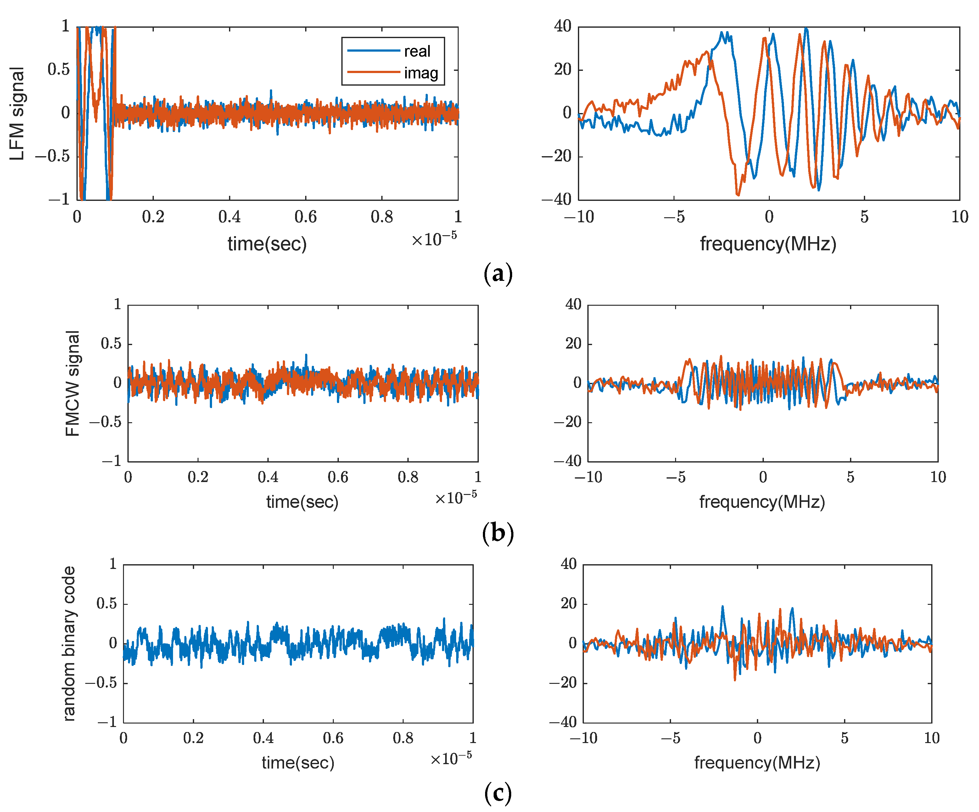
Compared with the pulse doppler radar using linear frequency modulated waveform (LFM), noise radar uses a continuous signal that appears to be random noise. Therefore, the average power can be very low, and the waveform is not deterministic. Figure 1 shows baseband signals: the LFM pulse, the frequency modulated continuous waveform (FMCW), and the random binary code. The time domain signal is shown on the left side, and the frequency domain signal is on the right side. The bandwidth is 10 MHz, and the average signal-to-noise ratio (SNR) is 10 dB for all. The duty cycle of the LFM pulse is 0.1.

The high power of the pulse and the pulse repetition provides characteristics to be easily detected. For the same noise level, the continuous waveforms can have lower power than the pulsed ones, which supports the LPD property. When the noise signal becomes large, this effect becomes significant. Moreover, random codes outperform continuous waveforms because they do not exhibit a deterministic pattern in the time and frequency domains and have no start or finish time.

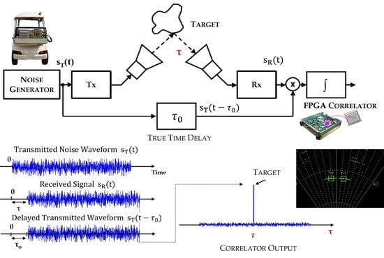
The biggest drawback of random noise radar is the complicated hardware, including the correlators. Figure 2 illustrates a noise radar, which consists of a noise signal generator, transmitter antenna, receiver antenna, and correlators in the receiver. Unlike other radars that use a predetermined waveform, the correlation must be performed with a real-time generated random signal, which requires real-time digital conversion of the transmitted signal. A random noise signal is generated by the thermal noise of an analog circuit, which is the genuine noise source, or by a digital pseudo-random sequence (PRS). The bandwidth in the PRS is defined as the minimum pulse width, and its generation is relatively simple.

2.1. Noise Waveform Generation

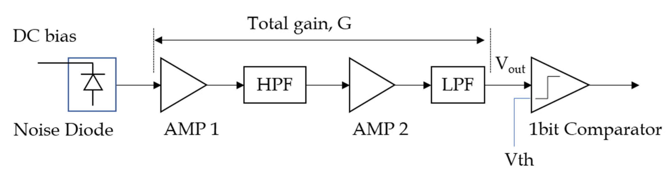
Analog noise generation is implemented by a diode, amplifier, filters, and 1-bit comparator, as shown in Figure 3. A high-pass filter (HPF) and a low-pass filter (LPF) determine the bandwidth. Considering the noise signal near the DC and amplifier gain characteristics, the cutoff frequencies of the HPF and LPF were set to 150 MHz and 1.2 GHz, respectively, to generate a one-sided bandwidth of 750 MHz. A 1-bit high-speed comparator converted the analog noise signal into digital signals. The conversion speed to handle the minimum pulse width is a few Giga samples per second (Gsps).

The gain of the amplifier can be expressed as the following equation.

$$\mathrm{G}=\frac{V_{out}}{\sqrt{{10}^{\left(0.1\times PSD\times BW-30\right)}\times R_{in}}}$$

(1)

where $PSD$ is the power spectral density of the noise diode [dBm/Hz], $BW$ is the bandwidth (Hz), $R_{in}$ is the input resistor, and $V_{out}$ is the root-mean-squared (RMS) value of the output voltage (V).

On the other hand, PRS is generated by FPGA using white Gaussian noise generator (WGNG) IP provided by Xilinx, which combines the Box–Muller algorithm and the central limit theorem to generate white Gaussian noise. The Box–Muller algorithm generates a variable with a normal distribution by transforming two independent random variables with uniform distributions [13].

2.2. Array Antenna and Wideband Beamforming with TTD

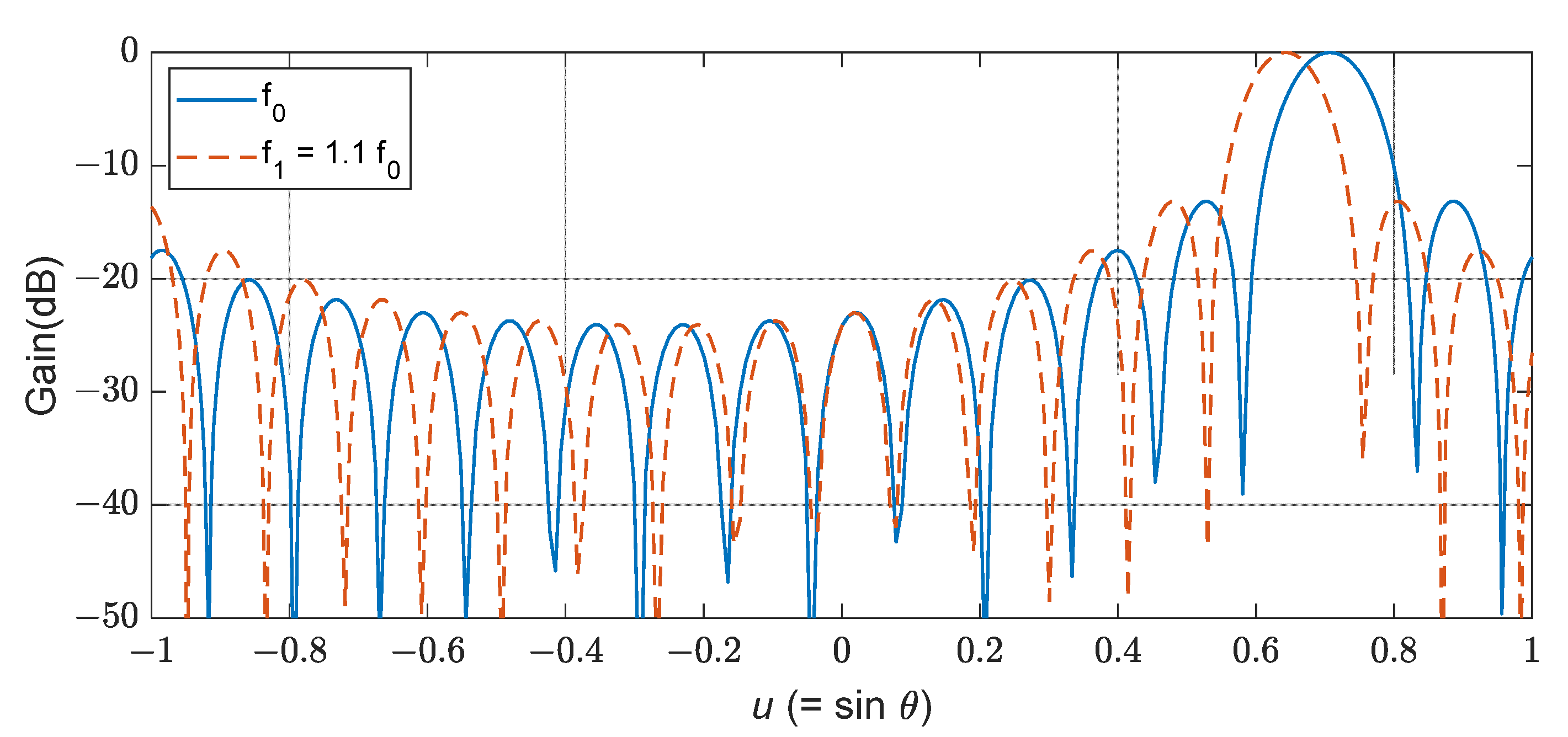
If the instantaneous bandwidth increases, the beamforming by the phase shifters squints the boresight angle, shifts nulls, increases the sidelobe level and widens the beamwidth. Consequently, the angle measurement performance becomes poor [14,15]. Thus, we adopted the true time delay to increase the bandwidth up to 15%.

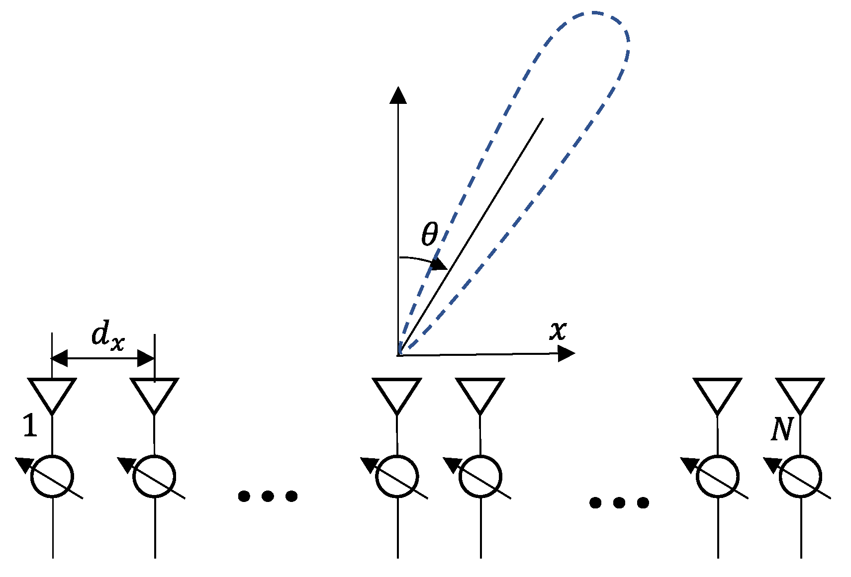
The detailed equations can be found in [10] and are summarized below. Normalized radiation pattern in the far-field with one-dimensional (1D) uniform arrays in Figure 4 is expressed as

$$E\left(\theta \right)=f\left(\theta \right){\displaystyle \sum }_n{a}_n\exp \left[jk\left(n{d}_{x}u\right)\right], k=\frac{2\pi }{\lambda }, u=\sin \theta ,$$

(2)

where $\theta$ is the input direction,$a_n$ is the complex weight of each array element, $d_x$ is the distance between the two arrays, and $f\left(\theta \right)$ is the pattern of each array, assuming that the patterns of all elements are equal. In the case of a single frequency, $a_n$ that maximizes the signal in the ${\theta }_0$ direction can be selected as follows:

$$a_n=\left|a_n\right|\exp \left(-j{k}_{0}n{d}_x{u}_0\right)=\left|a_n\right|\exp \left(-jn{\varphi }_0\right)$$

(3)

$${\varphi }_0=k_0{d}_x{u}_0,\hspace{1em}{u}_0=\sin {\theta }_0$$

(4)

Then, the array pattern is

$$F\left(\theta \right)={\displaystyle \sum }_n\left|a_n\right|\exp \left[jn{d}_x\left(ku-k_0{u}_0\right)\right].$$

(5)

The phase of the complex weight $a_n$ is typically implemented using a phase shifter with a value of $n{\varphi }_0$ for the nth array. This is because $k$ can be assumed to be constant for a single frequency or a narrow bandwidth. However, if the bandwidth increases and this assumption is no longer valid, the implementation by phase shifters results in a squint of the boresight angle, beam broadening, and so on. Figure 5 shows the squinted boresight angle for a 10% shifted frequency.

However, the TTD can maintain the pattern for a wide bandwidth because it employs the time delay of the actual path difference. The pattern is expressed by

$$F\left(\theta \right)={\displaystyle \sum }_n\left|a_n\right|\exp \left[j2\pi nf\left(\frac{d_{x}u}{c}-{\tau }_0\right)\right].$$

(6)

The time delay of two consecutive arrays is ${\tau }_0=d_{x}u/c$, and the maximum delay is $(N-1){\tau }_o$, which increases as the number of arrays increases. $d_x$ is typically chosen to be half of the wavelength. In this study, the radar is designed to operate in the X-band (10 GHz), and $d_x$ is half of the wavelength (0.015 m). To cover the maximum angle of 30° with 16 arrays, the maximum delay is 375 ns $(=d_x\sin {30}^{\mathrm{o}}/c\times 15)$. The TTD component used for beamforming is RMF040160PA from RFCORE, which operates at 4–16 GHz and contains a 6-bit TTD and a 6-bit digital step attenuator. The least significant bit (LSB) has a minimum delay period of 3.125 ps, which corresponds to 3.58° in the X-band. We utilized two in series to cover 30° because the maximum delay time was 197 ps.

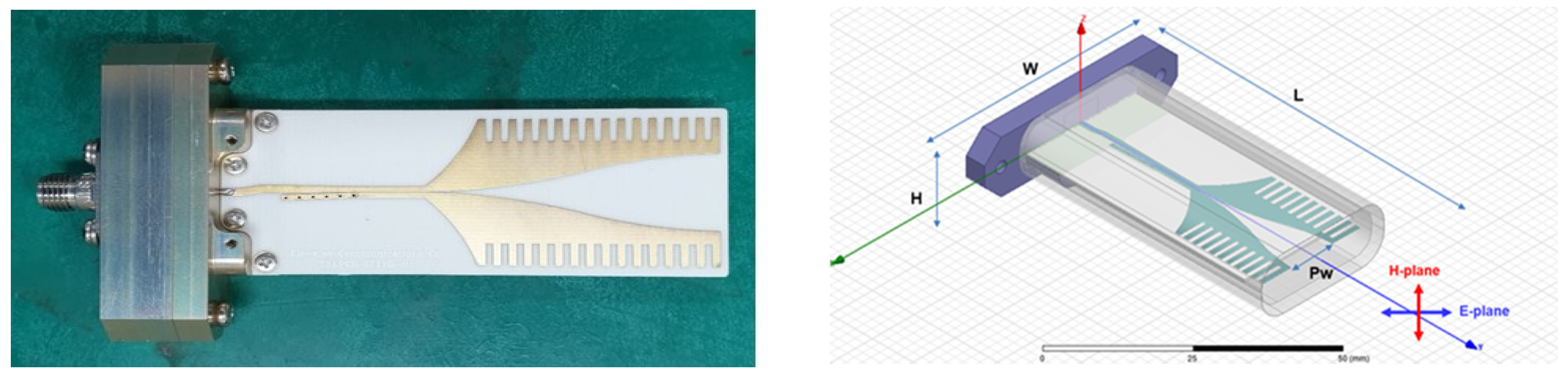
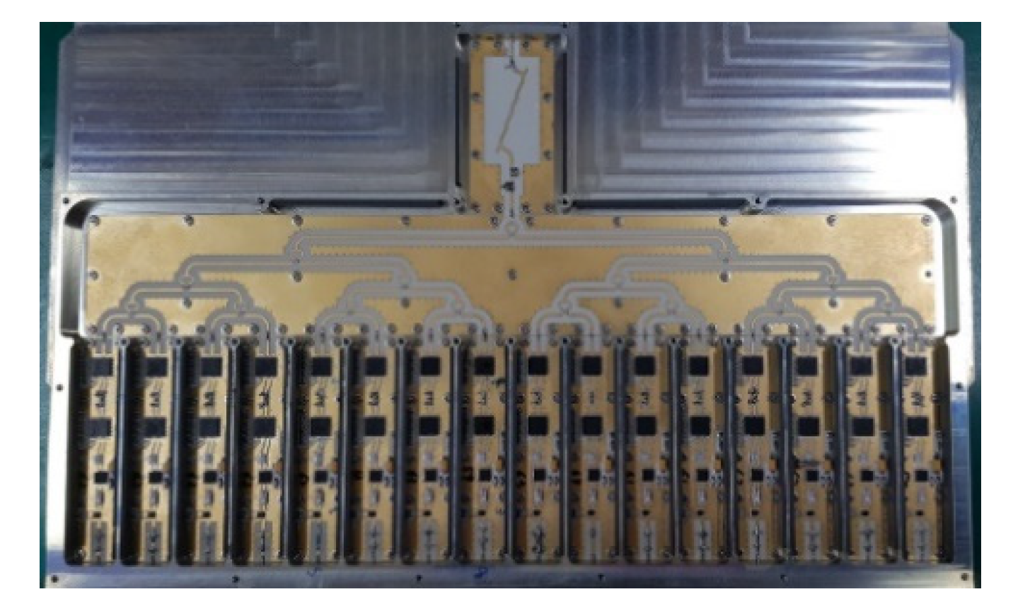
Figure 6 shows a photograph of the fabricated antenna. The substrate of the radiation element was Rogers RO4003C with a dielectric constant of 3.38 and a thickness of 0.5 mm, and the radome was made by Teflon with a dielectric constant of 2.1. The dimensions are 63.6 mm (L) × 46.0 mm (W) × 13.0 mm (H), with a Pw of 10 mm. The measured pattern will be provided in Section 3.

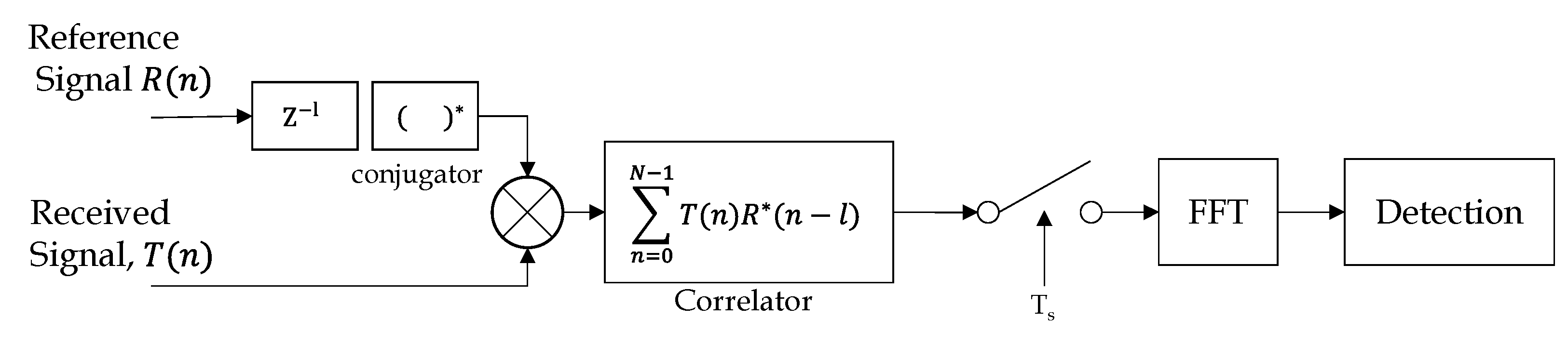
2.3. Digital Correlators and Resource Savings

The input of the correlator is data obtained by digitally converting the transmitted and received signals. The received signal is multiplied by the delayed transmitted signal and accumulated by N pieces of data [4].

$$y\left(l\right)={\displaystyle \sum }_{n=0}^{N-1}T\left(n\right)R^{*}\left(n-l\right) \left(l=1,\dots ,L\right)$$

(7)

where $R\left(n\right)$ is the reference transmitted signal, $T\left(n\right)$ is the received signal, * means the complex conjugate and L is the number of range cells and correlators. The sampling rate of the data, that is, the chip period $T_c$, is 0.666 ns (1.5 GHz), and the correlation time $T_s$ is 117 ms. Because the number of correlated data is 175,670, the gain is considerable such that low-power detection can be implemented. The correlators were developed in parallel using Xilinx’s Vertex 7 Series FPGA, shown in Figure 7. The number of correlators L, which is the primary factor affecting FPGA resources, determines the detection range.

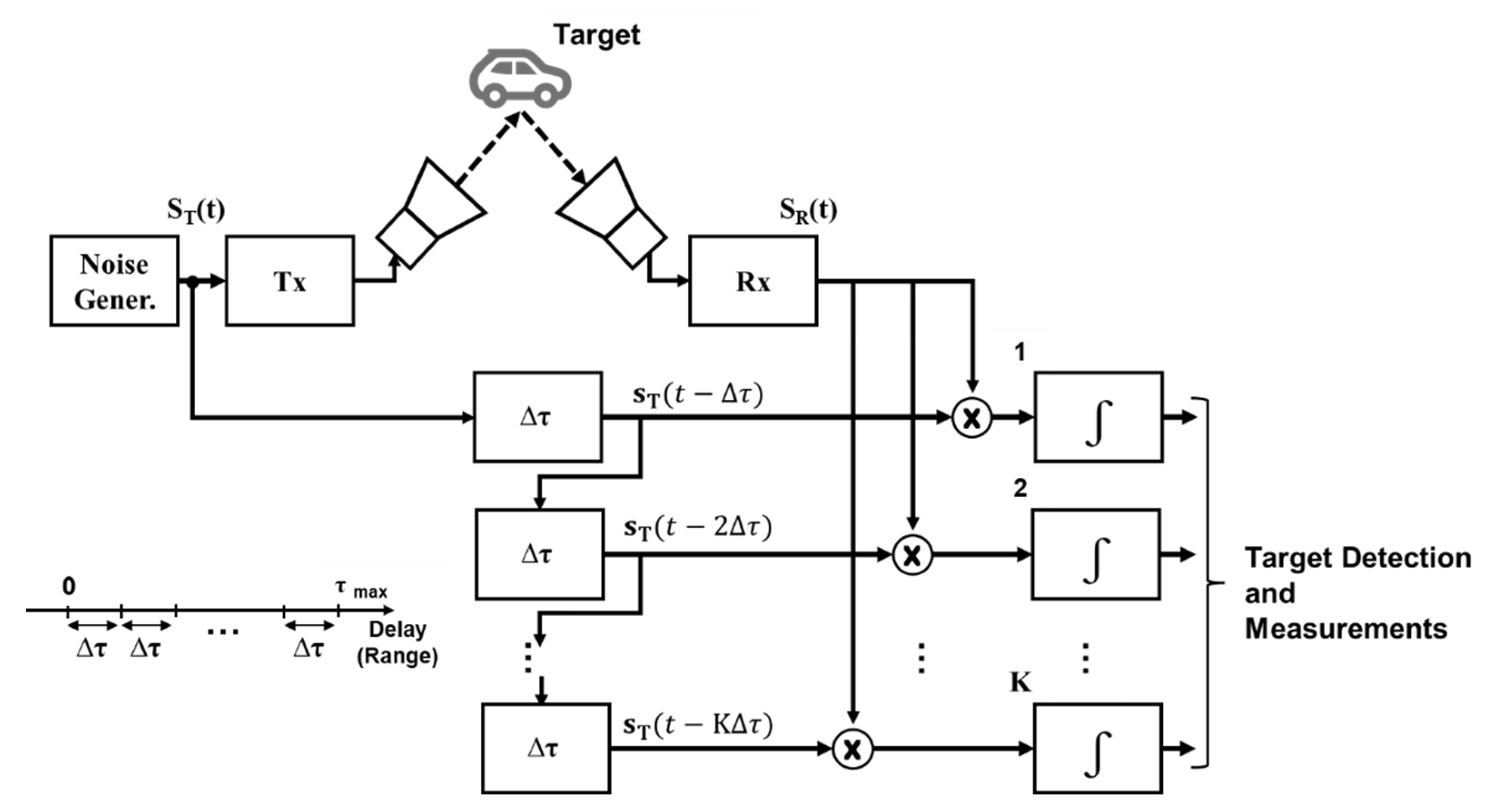
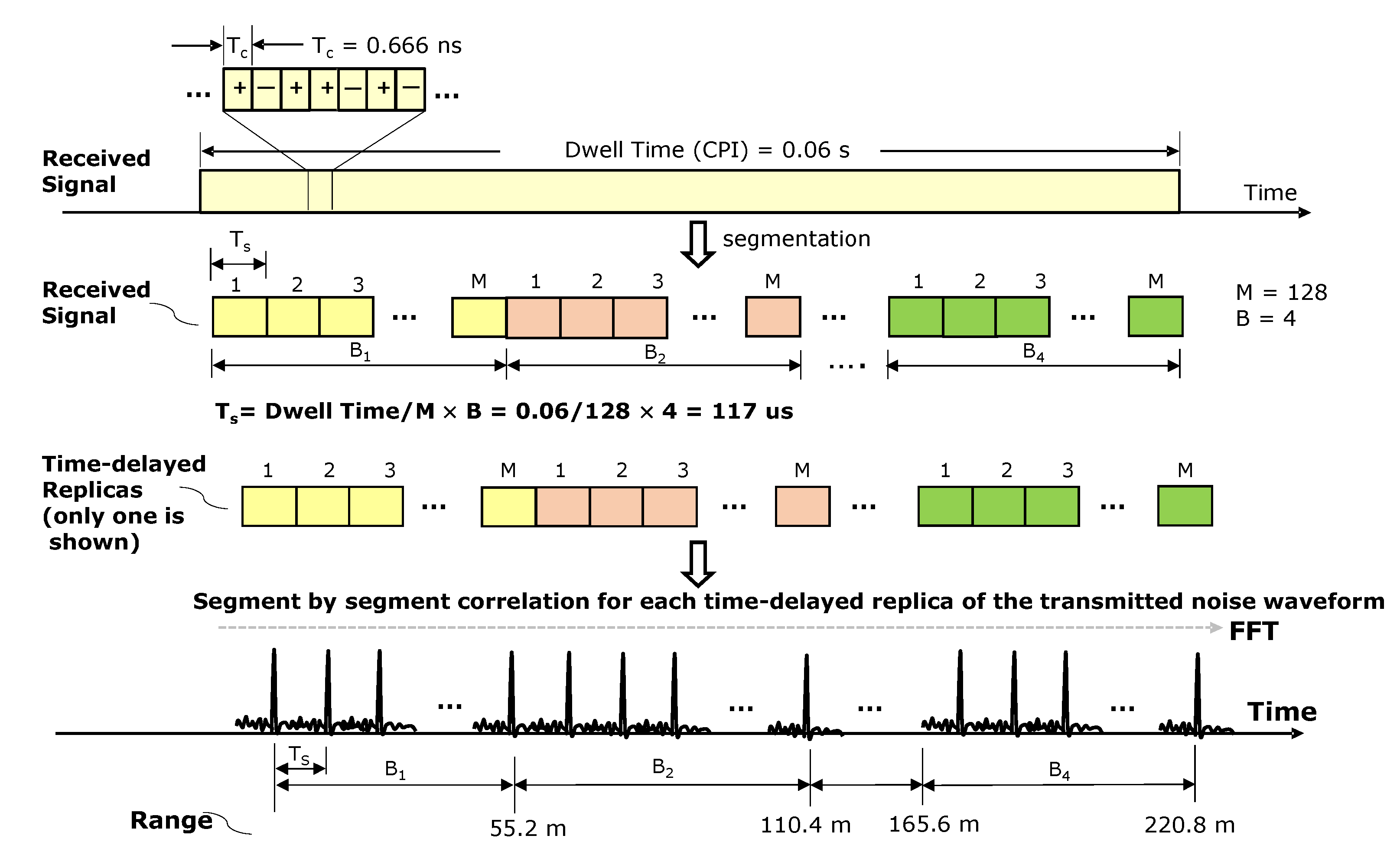
In this study, at least 2200 correlators are required to implement the 220 m range, which necessitates a significant amount of FPGA resources. To reduce these resources, we divided the distance into four ranges and processed them sequentially. That is, the time delays of the correlators are changed periodically over four times, covering a distance of 55.2 m at a time, as shown in Figure 8. With this method, we could reduce the FPGA resources by a quarter. For each quarter distance, the output of the correlator was doppler-processed 128 times in a digital signal processor (DSP). Constant false alarm rate (CFAR) detection was then performed. The whole processing chain is described in Figure 9.

3. System Development

3.1. Specification

Our X-band radar system has an instantaneous bandwidth of 1.5 GHz and an azimuth angle of 60° field of view (FOV). The maximum detection range and velocity are 200 m and 64 m/s, respectively. The specifications of the entire system are listed in

Table 1. System Specification.

Parameter	Value
Frequency	X-band
Instantaneous bandwidth	1.5 GHz
Transmit Power (average)	−14 dBm
Field of View	±30°
Maximum detection Range	220 m
Maximum detection velocity	±64 m/s
Sampling Rate (I/Q sampling)	1.5 Gs/s
Correlation Time	117 μs
Doppler FFT	128
Number of arrays	16

. The system consists of an array antenna unit, RF transceiver unit, and digital signal processing unit composed of FPGAs and a DSP.

3.2. Antenna and Transceiver

Figure 10 shows a photograph of the system. The antenna unit in Figure 11 has a dimension of 300 × 300 × 250 mm (W × D × H) and a weight of 7.24 kg. It includes a transmit/receive array antenna and beamformer with TTD. The transceiver (transmitter/receiver) unit has a dimension of 270 × 310 × 250 mm (W × D × H) and a weight of 17.98 kg. It includes a noise generator, frequency synthesis, downconverter, ADC, and correlator.

Figure 12 shows the antenna patterns of the measurement and simulation results. Measurements were performed using a near-field scanner (NFS) in an anechoic chamber. It was measured for the frequency range 9.25–10.75 GHz, overall steering angle from −30° to 30°. The average side lobe level was measured as 23.3 dB. The figure shows the simulated and measured antenna patterns at the highest (10.25 GHz) and lowest (9.25 GHz) frequencies for steering angles of 0° and 30°. The asymmetry of the measured pattern seems to be caused by the difference in the active components used for beam steering and tapering to lower the side lobe level. When passive components were included, the radiation pattern was very symmetrical. An angle squint did not occur, and the measurement results were comparable with the simulation.

The configurations of the antenna and transceiver units are shown in Figure 13. The antenna unit consists of a transmit beam steering assembly (TBSA) with the TTD, a transmitter array antenna with 16 radiating elements, receive beam steering assembly (RBSA), and a receiver array antenna with 16 elements. The RF signal from the transceiver was amplified and delayed for each channel in the TBSA, consisting of 16 channels. It is then radiated in the desired direction through the transmission array antenna. The signal reflected from the target was received by the receiving array antenna, amplified by the RBSA, and transferred to the transceiver.

A noise generation/up converter (NGUC) generates noise and converts it into an RF band. Figure 14 shows the measured frequency spectrum of the generated and PRS noises. The bandwidth was more than 15%, and the flatness was within 4 dB for both cases.

A low noise amp/down converter (LNDC) consists of receiving and reference channels for correlation processing of noise signals. The receiving channel blocks the transmission leakage power from the transmission antenna. It has a wide dynamic range for simultaneously processing a highly reflective signal from a distance of several meters and a low signal reflected from the maximum detection distance. The reference channel stably amplifies the reference noise signal provided by the NGUC. It prevents the reference signal, which has a relatively high power level, from leaking to the receiving channel.

In the digital converter/correlator (DCC) shown in Figure 15, the amplitude and phase are corrected for each channel data, and the DC offset is removed before the correlation to reduce the false target detections that may occur in the I/Q demodulator. The output of the correlators is transferred to the processing unit of the DSP using sFPDP packets of 2.5 Gbps in the optical lines.

The DSP performs Doppler FFT on the data from the correlators, detects the target, and displays it on the monitor.

4. Experiments

4.1. Experimental Setup

We installed the developed radar system on a small vehicle as shown in Figure 16 and conducted a field test. The test was conducted at the Korea Automobile Testing & Research Institute (KATRI). The site view is shown in Figure 17.

4.2. Results

Experiments were performed using corner reflectors with a radar cross-section (RCS) of 1 m². Figure 18 shows the range-Doppler map when the vehicle approached 20 km/h from 220 m at the antenna direction of 30°. The signals at zero velocity show the clutter.

Figure 19 shows the measured distance and velocity when approaching from 220 m to 40 m at 20 km/h. During the approach, the vehicle’s speed was observed to vary, which seems to include measurement errors and actual vehicle speed changes. We conducted five more experiments on situations of moving away from 20 km/h, moving away/approaching at 40 km/h, and moving away/approaching at 60 km/h, in addition to the case of approaching at 20 km/h.

The true values were unknown because sensors like GPS, which can measure distance and velocity with high accuracy, were not installed. Thus we did a linear regression for the distance and defined a distance error as the deviation of distance from the regression value. The velocity error was defined as the deviation from the mean value. Figure 20 shows the distance and velocity error from six experiments. As it is data from different experiments, even considering the fluctuations in speed, they could show the performance to some extent. The error increases with a distance above 100 m, which is due to the SNR. On the other hand, there is a degradation in accuracy at close range, which appears to be the effect of the clutter signal located near distance.

To test the range resolution, two corner reflectors were set up, as shown in Figure 21. The plan position indication (PPI) in Figure 22 displays the resolved targets 40 cm apart. Although the ideal resolution was 10 cm, the reliable resolution in the experiment was approximately 40 cm. This might be caused by hardware and processing restrictions. Other green lines are the objects on the site.

Next, two corner reflectors were installed in the azimuth direction to test the angular resolution and maximum coverage. The corner reflectors, as illustrated in Figure 23, were placed 8.54 m apart and detected by a radar approaching 35 m away. The beam width of the 16 array antennas was approximately 7°, which is supported by the pattern in Figure 11. In this test, two targets separated by twice the beam width were detected to test the practical resolution. Figure 24 shows the result.

Finally, Figure 25 shows the PPI display for two corner reflectors spaced 30 m apart, indicating the angular coverage.

5. Conclusions

In this study, an X-band noise radar with 15% bandwidth was developed. A TTD was applied to correct the distortion of the beam pattern owing to the wideband, and correlators were implemented by high-speed parallel processing through the FPGA. In addition, by employing the time-division method, the FPGA’s computational resources for implementing correlators were reduced to a fourth.

The angular resolution was rather low compared with the range resolution because the X-band was chosen. In the future, it will be necessary to choose a higher frequency band to increase the angular resolution without expanding the physical size of the radar, which can also increase the range resolution.

We expect that the use of noise radar will increase because of its low detectability and low interference properties, particularly in environments where multiple radars operate in the same band, as well as in military radars.

References

1. Savci, K.; Stove, A.G.; De Palo, F.; Erdogan, A.Y.; Galati, G.; Lukin, K.A.; Wasserzier, C. Noise radar—Overview and recent developments. IEEE Aerosp. Electron. Syst. Mag. 2020, 35, 8–20. [Google Scholar] [CrossRef]
2. Lukin, K.A.; Mogyla, A.A.; Palamarchuk, V.P.; Vyplavin, P.L.; Zemlyaniy, O.V.; Shiyan, Y.A.; Zaets, M. Ka-band bistatic ground-based noise waveform SAR for short-range applications. IET Radar Sonar Navig. 2008, 2, 233–243. [Google Scholar] [CrossRef]
3. Lukin, K.A.; Mogila, A.A.; Vyplavin, P.L.; Palamarchuck, V.P.; Zaets, N.K.; Zemlyany, O.V. Reconfigurable Ground Based Noise-Waveform-SAR for Short Range Applications. In Proceedings of the 7th European Conference on Synthetic Aperture Radar, VDE, Friedrichshafen, Germany, 2–5 June 2008; pp. 1–4. [Google Scholar]
4. PACE; Phillip, E. Detecting and Classifying Low Probability of Intercept Radar; Artech House: Norfolk County, MA, USA, 2009. [Google Scholar]
5. Yan, H.; Boljanovic, V.; Cabric, D. Wideband millimeter-wave beam training with true-time-delay array architecture. In Proceedings of the 53rd Asilomar Conference on Signals, Systems, and Computers, Pacific Grove, CA, USA, 3–6 November 2019; IEEE: Piscataway, NJ, USA, 2019. [Google Scholar]
6. Hashemi, H.; Chu, T.S.; Roderick, J. Integrated true-time-delay-based ultra-wideband array processing. IEEE Commun. Mag. 2008, 46, 162–172. [Google Scholar] [CrossRef]
7. Haupt, R.L. Fitting time delay units in a large wideband corporate fed array. In Proceedings of the 2013 IEEE Radar Conference (RadarCon13), Ottawa, ON, Canada, 29 April–3 May 2013; IEEE: Piscataway, NJ, USA, 2013. [Google Scholar]
8. Iezekiel, S.; Burla, M.; Klamkin, J.; Marpaung, D.; Capmany, J. RF engineering meets optoelectronics: Progress in integrated microwave photonics. IEEE Microw. Mag. 2015, 16, 28–45. [Google Scholar] [CrossRef]
9. Boljanovic, V.; Yan, H.; Lin, C.C.; Mohapatra, S.; Heo, D.; Gupta, S.; Cabric, D. Fast beam training with true-time-delay arrays in wideband millimeter-wave systems. IEEE Trans. Circuits Syst. I Regul. Pap. 2021, 68, 1727–1739. [Google Scholar] [CrossRef]
10. Robert, J. Mailloux. In Phased Array Antenna Handbook, 3rd ed.; Artech House: Norfolk County, MA, USA, 2018. [Google Scholar]
11. Talisa, S.H.; O’Haver, K.W.; Comberiate, T.M.; Sharp, M.D.; Somerlock, O.F. Benefits of digital phased array radars. Proc. IEEE 2016, 104, 530–543. [Google Scholar] [CrossRef]
12. Liu, M.; Zou, L.; Wang, X. Practical beamforming technologies for wideband digital array radar. Prog. Electromagn. Res. Lett. 2019, 86, 145–151. [Google Scholar] [CrossRef] [Green Version]
13. Ghazel, A.; Boutillon, E.; Danger, J.L.; Gulak, G.; Laamari, H. Design and Performance Analysis of a High Speed AWGN Communication Channel Emulator. In Proceedings of the IEEE PACRIM Conference, Victoria, BC, Canada, 21–23 August 2001. [Google Scholar]
14. Rotman, R.; Tur, M. Wideband phased arrays with true time delay beamformers challenges and progress. In Proceedings of the 8th European Conference on Antennas and Propagation (EuCAP 2014), The Hague, The Netherlands, 6–11 April 2014; IEEE: Piscataway, NJ, USA, 2014; pp. 743–744. [Google Scholar]
15. Dyadyuk, V.; Huang, X.; Stokes, L.; Pathikulangara, J. Implementation of wideband digital beam forming in the E-band: Towards a hybrid array. In Proceedings of the 40th European Microwave Conference, Paris, France, 28–30 September 2010; IEEE: Piscataway, NJ, USA, 2010; pp. 914–917. [Google Scholar]
Figure 1. Comparison among three waveforms: LFM pulse, FMCW, and random code. (a) LFM pulse; (b) FMCW signal; (c) Random binary code.
Remotesensing 14 04489 g001
Figure 2. Configuration of the Noise Radar.
Remotesensing 14 04489 g002
Figure 3. Baseband true noise generation block.
Remotesensing 14 04489 g003
Figure 4. 1D array antenna.
Remotesensing 14 04489 g004
Figure 5. Comparison of the beampatterns of two frequencies.
Remotesensing 14 04489 g005
Figure 6. Fabricated Antenna.
Remotesensing 14 04489 g006
Figure 7. FPGA correlators.
Remotesensing 14 04489 g007
Figure 8. Processing sequences reducing FPGA resources.
Remotesensing 14 04489 g008
Figure 9. Signal processing chain.
Remotesensing 14 04489 g009
Figure 10. Antenna and Transceiver.
Remotesensing 14 04489 g010
Figure 11. Antenna Unit.
Remotesensing 14 04489 g011
Figure 12. Beam pattern of antenna at the end frequencies (9.25 and 10.75 GHz) for steering angles of 0° (up) and 30° (down).
Remotesensing 14 04489 g012
Figure 13. Configuration of the antenna and transceiver units.
Remotesensing 14 04489 g013
Figure 14. Noise spectrum: Thermal noise (left) and PRS noise (right).
Remotesensing 14 04489 g014
Figure 15. Digital correlator (left) and DSP signal processing board (right).
Remotesensing 14 04489 g015
Figure 16. Test vehicle (Front and Back view).
Remotesensing 14 04489 g016
Figure 17. Test site view.
Remotesensing 14 04489 g017
Figure 18. Range-Doppler map of a target moving at 20 km/h.
Remotesensing 14 04489 g018
Figure 19. Measured distance and velocity when approaching at 20 km/h.
Remotesensing 14 04489 g019
Figure 20. Distance and velocity errors according to the distance.
Remotesensing 14 04489 g020
Figure 21. Test setup for measuring the range resolution.
Remotesensing 14 04489 g021
Figure 22. PPI display showing the range resolution.
Remotesensing 14 04489 g022
Figure 23. Test setup for measuring the angular resolution.
Remotesensing 14 04489 g023
Figure 24. PPI display showing the angular resolution.
Remotesensing 14 04489 g024
Figure 25. PPI display showing the angular coverage.
Remotesensing 14 04489 g025