SORAG: Synthetic Data Over-Sampling Strategy on Multi-Label Graphs

Abstract

In many real-world networks of interest in the field of remote sensing (e.g., public transport networks), nodes are associated with multiple labels, and node classes are imbalanced; that is, some classes have significantly fewer samples than others. However, the research problem of imbalanced multi-label graph node classification remains unexplored. This non-trivial task challenges the existing graph neural networks (GNNs) because the majority class can dominate the loss functions of GNNs and result in the overfitting of the majority class features and label correlations. On non-graph data, minority over-sampling methods (such as the synthetic minority over-sampling technique and its variants) have been demonstrated to be effective for the imbalanced data classification problem. This study proposes and validates a new hypothesis with unlabeled data over-sampling, which is meaningless for imbalanced non-graph data; however, feature propagation and topological interplay mechanisms between graph nodes can facilitate the representation learning of imbalanced graphs. Furthermore, we determine empirically that ensemble data synthesis through the creation of virtual minority samples in the central region of a minority and generation of virtual unlabeled samples in the boundary region between a minority and majority is the best practice for the imbalanced multi-label graph node classification task. Our proposed novel data over-sampling framework is evaluated using multiple real-world network datasets, and it outperforms diverse, strong benchmark models by a large margin.

1. Introduction

Graphs are becoming ubiquitous across a large spectrum of real-world applications in the form of social networks, citation networks, telecommunication networks, biological networks, etc. [1]. In addition, numerous applications involving multimedia, such as video surveillance, video streaming, healthcare systems, and intelligent indoor security systems depend on using graphs as research objects [2,3,4]. For a considerable number of real-world graph node classification tasks, the training data follow a long-tail distribution, and node classes are imbalanced. In other words, each of a few “majority” classes has a large number of samples, while most classes only contain a handful of instances. Taking the NCI chemical compound graph as an example, only approximately 5% of molecules are labeled as active in the anticancer bioassay test [5]. Graph node classification tasks are often further complicated by the fact that graph nodes can be associated with multiple labels in many real-world network data. Many social media sites, such as BlogCatalog, Flickr, and YouTube, allow users to use a diverse set of labels representing their various interests. A person can join several interest groups on Flickr, such as Landscape and Travel, and different video genres on YouTube, such as Cooking and Wrestling. Furthermore, many networks are characterized by imbalanced label distribution and multi-label nodes at the same time, as shown in Figure 1.

To date, a large body of work has focused on graph representation learning (GRL) with balanced node classes and simplex labels [8,9,10,11,12]. However, these models do not perform well when graphs exhibit the aforementioned characteristics of being imbalanced and multi-label for the following reasons. (1) The problem caused by the imbalanced setting: The imbalanced data make the classifier overfit the majority class, and the features of the minority class cannot be sufficiently learned [13]. Furthermore, the above problem is aggravated by the presence of the topological interplay effect [5] between graph nodes, making the feature propagation dominated by the majority classes. (2) The problem caused by the multi-label setting: Multi-label graph architectures typically encode very complex interactions between nodes with shared labels [5], which is challenging to capture. Therefore, it is essential to develop a specific graph learning method for class imbalanced multi-label graph data. However, research in this direction is still in its infancy. Thus, in this study, we propose imbalanced multi-label GRL to address this challenge while also contributing to graph learning theory.

For imbalanced data, minority over-sampling is an effective measure to improve the classification accuracy [14,15,16]. This strategy has recently been confirmed to be effective for graph data as well [17]. Traditional over-sampling techniques consist of a two-step process: (1) the selection of some minority instances as “seed examples”; (2) the generation of synthetic data with features and labels similar to the seed examples, which are then added to the training data. For example, the most popular over-sampling technique—the synthetic minority over-sampling technique (SMOTE) [14]—addresses the problem of minority generation by performing interpolation between randomly selected minority instances and their nearest neighbors. Cost-sensitive learning is another type of effective approach for alleviating the problem of imbalanced data applied to a classification [16], where the basic assumption is that the cost resulting from different types of misclassification varies significantly (e.g., the cost of treating an intruder as a non-intruder is much greater than treating a non-intruder as an intruder). The principle of applying cost-sensitive learning methods to imbalanced learning problems is to assign a larger penalty cost to misclassified minority class samples [18]. Existing cost-sensitive classification algorithms can generally be grouped into three categories [19]: algorithms that (1) pre-process the training data, (2) post-process the output, and (3) apply direct cost-sensitive learning methods. Data pre-processing aims to make the classification results on the new training set equivalent to cost-sensitive classification decisions on the original training set, typically along the lines of sampling [18] and weighting [16]. Post-processing the output makes the classifier biased toward minority classes by adjusting the classifier decision threshold, as represented by MetaCost [20] and ETA [21]. Direct cost-sensitive learning methods embed the cost information into the objective function of the learning algorithm to obtain the minimal expected cost, such as cost-sensitive decision trees [22] and cost-sensitive SVM [23].

However, mainstream over-sampling techniques have significant shortcomings when applied to graph data, as the selection of seed examples prioritizes global minority nodes while ignoring local minority nodes, and each synthetic instance is always assigned a label based on some specific strategy, which may be incorrect. This is because, in contrast to non-graph data, the relationships between graph nodes are explicitly expressed by the edges connecting them, meaning that the representation learning of a node can be heavily dependent on its neighboring unlabeled nodes through the feature propagation mechanism inherent to graphs.

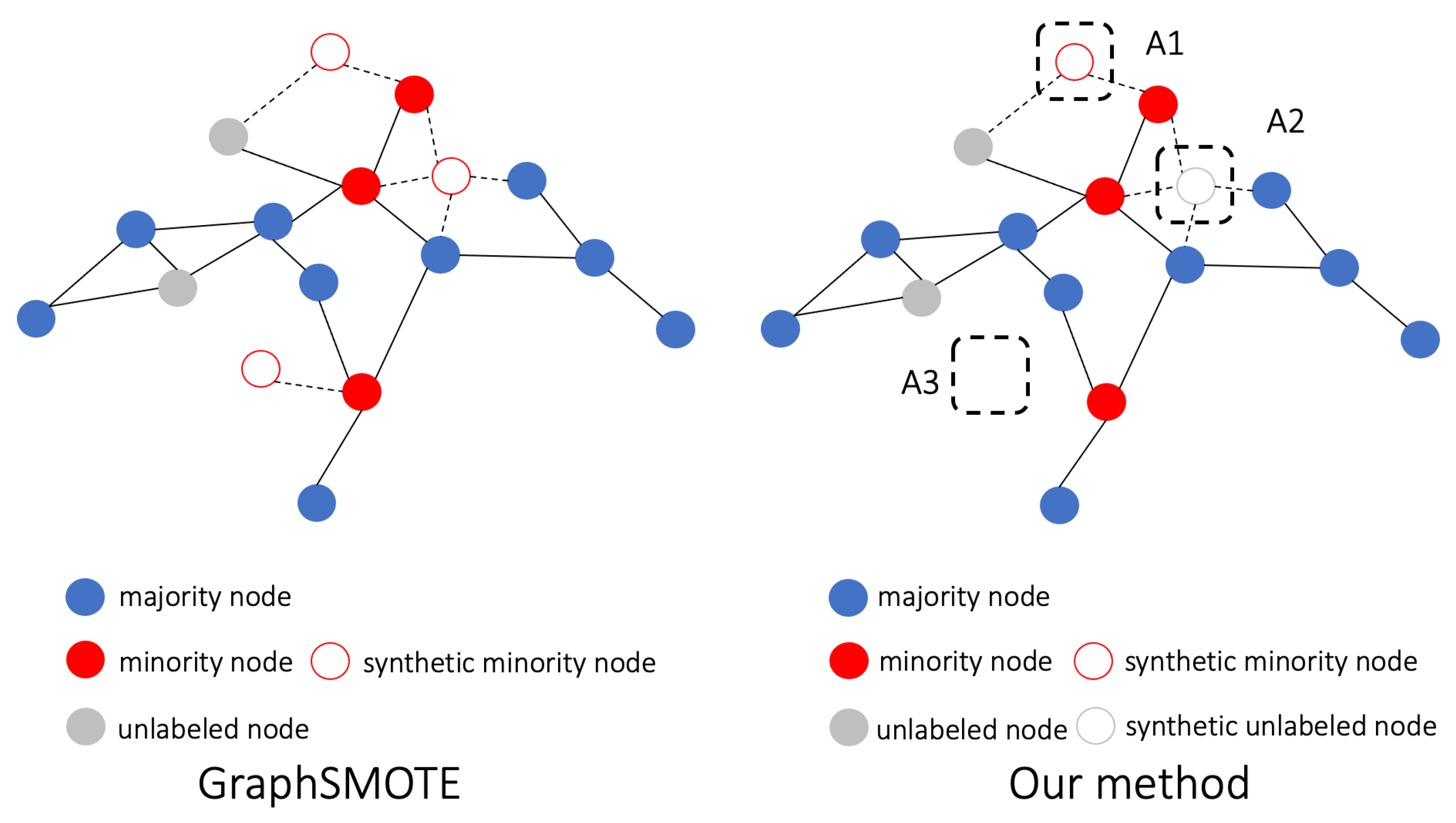
Motivated by the above observations, we propose and test the following hypothesis. In addition to synthetic minority samples, synthetic unlabeled samples can also facilitate the debiasing of graph neural networks (GNNs) on an imbalanced training set. In particular, for nearby global minority samples that are a local majority, we can “safely” produce virtual samples of the same class and add them into the training sets to balance the class distribution. Global minority samples that are also a local minority are more likely to be local outliers, and thus, they are risky for selection as seed examples for further over-sampling. For nearby global minority samples whose neighbors are class-balanced, it is difficult to determine the labels of virtual samples. Thus, the production of unlabeled virtual nodes should be encouraged, which can help minorities by “blocking” the over-aggregation of the majority features delivered through edges. This idea is illustrated in Figure 2. We argue that the key to over-sampling on an imbalanced multi-label graph is to flexibly combine the synthesis of both labeled and unlabeled instances enriched by label correlations.

We extend the existing over-sampling algorithms to a novel framework for the imbalanced multi-label graph node classification task based on the above considerations. We extend the classic global minority-based seed example selection to the local minority perspective (see Section 3.2). Distinct from interpolation, which is commonly used in mainstream over-sampling techniques [24], we use a generative adversarial network (GAN) [25] to generate new instances. As a representative deep generative model, a GAN can capture label correlation information by estimating the probability distribution of seed examples [26]. We propose an ensemble architecture of a GAN and conditional GAN (CGAN) [27] for the flexible generation of both unlabeled and labeled synthetics (see Section 3.3). To make use of the graph topology information, we propose a method to obtain new edges between the generated samples and existing data with an edge predictor (see Section 3.4). The augmented graph is finally sent to a graph convolutional network (GCN) [12] for representation learning, together with the learned label correlations (see Section 3.5). We name our proposed framework SORAG, abbreviated from Synthetic data Oversampling StRAtegy on Graph.

In summary, our contribution is three-fold:

• We study an unexplored and novel research problem. We advance the traditional simplex-label graph learning to an imbalanced multi-label graph learning setting, which has diverse real-world applications (e.g., long-tailed graph node classification, link prediction, community detection, and ranking). To the best of our knowledge, this study is the first to focus on this task.
• We propose a new, general, and efficient GNN that addresses the deficiencies of previous graph over-sampling methods. Our framework flexibly ensembles the synthesis of labeled and unlabeled nodes to support the minority classes and leverage label correlations to generate more natural nodes.
• Extensive experiments on multiple standard real-world datasets demonstrate the high effectiveness of our approach. Compared with the current state-of-the-art model GraphSMOTE [17], our method has an improvement of 1.5% in terms of Micro-F1 and 3.3% in terms of Macro-F1 on average. The experimental results demonstrate the high effectiveness of the proposed approach. Detailed analyses of SORAG under different experimental environments and parameters are also presented.

2. Related Works

2.1. Graph Representation Learning

A growing number of applications use non-Euclidean methods to generate data, which are then represented as graphs with complex relationships and inter-object dependencies. Past feature representation and extraction algorithms face substantial difficulties in handling the complexity of graph data. Over the past decade, many studies on extending traditional feature extraction approaches for graph data have emerged. Among them, GRL has evolved considerably and can be roughly divided into three generations, including traditional graph embedding, modern graph embedding, and deep learning on graphs. The first generation of methods are classic dimension reduction techniques, such as IsoMap [28] and LLE [29]. The second generation of feature extraction methods on graphs are modern graph embedding methods, such as DeepWalk [30] and LINE [31]. GNNs can be broadly regarded as the third (and latest) generation of GRL after the traditional and modern graph embedding, and they are reported to achieve the most promising performance in a wide range of computational tasks on graphs [32].

A growing body of research has shown that GNNs are extremely effective for both traditional GRL tasks (e.g., recommender systems and social network analysis) and new research areas (e.g., healthcare, physics, and combinatorial optimization) [32]. A typical GNN consists of graph filters and/or graph pooling layers. The former take the node features and graph structure as inputs and output new node features. The latter take the graph as an input and output a coarsened graph with a few nodes.GNNs can be broadly classified into spatial and spectral approaches based on their graph filters. The former explicitly leverages the graph structure, for example, spatially close neighbors, whereas the latter analyzes the graph using a graph Fourier transform and an inverse graph Fourier transform [33].

Classical spatial-based GNNs include [9,10,11,34,35,36,37]. Ref. [9] is a very early GNN that uses the local transition function as a graph filter. A GraphSAGE filter [10] uses different aggregators (mean/LSTM/pooling) to aggregate information regarding the one-hop neighbors of the nodes. In addition, a GAT-filter [11] relies on a self-attention mechanism to distinguish the importance of neighboring nodes during the aggregation process. An ECC-filter [34] was also proposed to handle graphs with different types of edges. Similarly, a GGNN-filter [36] was designed for graphs with different types of directed edges. By contrast, a Mo-filter [35] is based on a Gaussian kernel. Finally, an MPNN [37] is a more general framework, with the GraphSAGE-filter and GAT-filter mentioned above being special cases. In general, spatial-based GNNs are more generalized and flexible.

Spectral-based graph filters use the graph spectral theory in the design of the filtering operations within the spectral domain. Early studies [33] dealt with the eigen decomposition of the Laplacian matrix and the matrix multiplication between dense matrices; thus, they are computationally expensive. To overcome this problem, a Poly-filter [38] based on a K-order truncated polynomial was proposed. To solve the problem of a Poly-filter in which the basis of the polynomial is not orthogonal, a Cheby-filter [38] based on the Chebyshev polynomial was introduced. A GCN-filter [12] is a simplified version of a Cheby-filter. The latter involves a K-hop neighborhood of a node during the filtering process, whereas in the former, K = 1. A GCN-filter can also be regarded as a spatial-based filter. Currently, GCNs are among the most widely used types of GNN. In our model, we used a GCN as the key component.

Feature extraction methods such as graph embedding and graph kernel techniques are strongly related to the study on GNNs. Compared to GNNs, the former only focus on representing network nodes as low-dimensional vector representations without targeting subsequent tasks, such as graph node classification and link prediction. Many graph embedding techniques are linear and not in an end-to-end manner, such as random walk [39] and matrix factorization [40]. Graph kernel techniques employ a kernel function to obtain the vector representations of graphs. They are also an important type of approaches to solve the graph classification problem. However, compared to GNNs, they are not learnable and far less efficient.

GNNs are designed for different graph-based tasks, such as node classification, link prediction, graph classification, and community detection. In particular, our task is semi-supervised, which means that we need to learn the representation of all nodes from a few labeled nodes and the remaining unlabeled nodes. GNNs are a rapidly growing field at the present time. For a more comprehensive and detailed introduction to this field, we refer the reader to [32].

2.2. Imbalanced Learning

If the classification classes are not approximately equal, and a few classes contain many more samples than the others, the dataset is called imbalanced. Representative techniques to handle imbalanced datasets include sampling methods, ensemble algorithms, and cost-sensitive approaches.

Re-sampling the original dataset is a strategy for balancing the majority and minority classes at the data level. This type of method constructs a well-balanced training set by over-sampling the minority class or under-sampling the majority class during the pre-processing step. Following that, any learning algorithm might be trained on the new dataset to reduce the system’s bias towards the majority classes. A typical example of sampling models is SMOTE [14]. To shift the learning bias toward the minority class, it generates synthetic samples depending on their nearest neighbors. Numerous extensions using various distance measures or selection criteria of seed samples are proposed based on the regular SMOTE algorithm. Among them, representative methods include the borderline SMOTE [41], the safe-level SMOTE [42], and the density-based SMOTE [43].

The methods of over-sampling and under-sampling are not limited to any modeling algorithm, which could be essentially regarded as data pre-processing processes. Ensemble classifiers and cost-sensitive approaches, which are algorithm-specific, could also be used to address data imbalance concerns as algorithm-level enhancement. The former type of method includes diverse hybrid sampling/boosting algorithms, such as SMOTEBoost [44], random under-sampling boost (RUSB) [45], and the balance cascade approach [46]. Besides the boosting algorithms, other ensemble methods such as balanced random forest [47] can also be applied for imbalanced datasets. Cost-sensitive approaches, which penalize the misclassification of the minority more severely, have also been reported to be effective in addressing the problem of class imbalance. Two popular examples of them are AdaCost [48] and weighted random forest [47].

2.3. Connections to Our Work

The focus of this study is to investigate solutions for semi-supervised GRL and graph node classification on imbalanced multi-label graphs. The most closely related works can be found in the emerging area of imbalanced graph node classification [5,17,49]. Among these works, the dual-regularized graph convolutional network (DR-GCN) [5] model relies on a class-conditioned adversarial training process to facilitate the separation of labeled nodes and the identification of minority class nodes. GraphSMOTE [17] attempts to transfer the classical SMOTE method [14], which deals with imbalanced data, to graph data. In addition, the relaxed GCN network (RECT) [49] has reported the best performance on imbalanced graph node classification tasks, and its core idea is based on the design and optimization of a class-semantic-related objective function. Unlike GraphSMOTE, which is based on labeled minority generation, we present the first graph node over-sampling model that utilizes synthetic unlabeled nodes to inhibit the tendency of GNNs to overfit to majority under the topological effect. The new supervision information resulting from labeled synthetics and the blocking of over-propagated majority features by unlabeled synthetics facilitates balanced learning between different classes, taking advantage of the strong topological interdependence between nodes on a graph. We specify the details of the proposed model in the next section.

3. Methodology

3.1. System Overview

An illustration of the proposed framework SORAG is shown in Figure 3. SORAG is composed of four components: (1) the first part is in charge of determining the global minority degree (GMD) and local minority degree (LMD) of each node and constructing training data (i.e., seed examples) for the virtual node generator; (2) the second part, the node generator, is an ensemble of a GAN [25] network and a CGAN [27] network, where the GAN is responsible for creating unlabeled nodes and the CGAN is used for generating labeled nodes; (3) the third component is an edge generator. Its job is to create virtual edges between the synthetic and real nodes so that the generated nodes can participate in the message passing on the graph more effectively; (4) finally, a GCN-based node classifier is designed for learning the node representations of the augmented graph as well as the inter-label dependencies for multi-label node classification. We elaborate on each component as follows.

3.2. Imbalance Measurement

In multi-label learning, a commonly used measure that evaluates the global imbalance of a particular label is IRLbl. Let $|C_i|$ be the number of instances whose i-th label value is 1; IRLbl is then defined as follows:

$$IRLb{l}_j=\frac{max\left\{|c_1|,|c_2|,\dots ,|c_m|\right\}}{c_i}.$$

(1)

Therefore, the larger the value of IRLbl for a label, the more minority class it is. For a node $v_i$, its GMD is defined as follows:

$$GM{D}_i=\frac{IRLb{l}_j·[B_{ij}=1]}{{\sum }_{j=1}^m[B_{ij}=1]},$$

(2)

where $[B_{ij}=1]$ means $v_i$ has the j-th label, and ${\sum }_{j=1}^m[B_{ij}=1]$ counts the number of labels that $v_i$ has.

The LMD of a node can be measured by the proportion of opposite class values in its local neighborhood. For $v_i$, let $N_i^k$ denote its k-hop neighbor nodes. Then, for label $c_j$, the proportion of neighbors having an opposite class to the class of $v_i$ is computed as

$$S_{ij}=\frac{{\sum }_{v_m\in N_i^k}[B_{ij}\ne B_{mj}]}{|N_i^k|},$$

(3)

where $S\in {\mathbb{R}}^{n\times m}$ is a matrix defined to store the local imbalance of all nodes for each label. Given S, a straightforward way to compute the LMD for $v_i$ is to average its $S_{ij}$ for all labels as follows:

$$LM{D}_i=\frac{{\sum }_{j=1}^m{S}_{ij}[B_{ij}=g_j]}{m},$$

(4)

where $g_j\in \{0,1\}$ denotes the minority class of the j-th label. Namely, if $|c_j|\ge 0.5·n$, $g_j=1$; otherwise, $g_j=0$. Here, n is the total number of vertices. Further, we group the global minority nodes into different types based on the LMD, and each type is identified correctly by the classifier with different difficulties. Following [50,51], we discretize the range [0, 1] of $LM{D}_i$ to define four types of nodes, namely safe (SF), borderline (BD), rare (RR), and outlier (OT), according to their local imbalance:

• SF: $0\le LM{D}_i<0.3$. Safe nodes are basically surrounded by nodes containing similar labels.
• BD: $0.3\le LM{D}_i<0.7$. Borderline nodes are located in the decision boundary between different classes.
• RR: $0.7\le LM{D}_i<1.0$. Rare nodes are located in a region overwhelmed by different nodes and are distant from the decision boundary.
• OT: $LM{D}_i=1.0$. Outliers are totally connected to different nodes.

Based on the above categories, we are confident about generating new virtual samples for the global minority samples belonging to SF by imitating their features and labels to balance the distorted class distribution. The global minority samples belonging to BD are located in the decision boundary; hence, it is challenging to determine the label for virtual samples similar to them. Therefore, we keep the new samples unlabeled and use them to weaken the over-propagation of majority class features by taking advantage of the feature smoothing mechanism on the graph. The global minority samples belonging to RR/OT are more likely to be outliers and should not be selected as seeds to generate new samples.

Furthermore, for $v_i$, we define two metrics: labeled seed probability (LSP) and unlabeled seed probability (USP) to describe the probability of being selected as a seed example to generate labeled synthetic nodes and unlabeled synthetic nodes, respectively. The seed probabilities (LSP/USP) are calculated as follows:

$$S{P}_i=GM{D}_i·LM{D}_i=\left\{\begin{array}{c}LS{P}_i,\mathrm{if}{v}_i\in \mathrm{SF}\hfill \\ US{P}_i,\mathrm{if}{v}_i\in \mathrm{BD}\hfill \end{array}\right.$$

(5)

We compute the LSP and USP scores for all nodes and sort them in descending order. The top-ranked nodes (controlled by the hyper-parameter seed example rate $\rho$) will be selected as seed examples. A min-max normalization processes all the GMD and LMD scores to improve the computation stability.

3.3. Node Generator

We denote the joint distribution of node feature x and label y in the SF region as $P_{SF}(x,y)$, the marginal distribution of y as $P_{SF}\left(y\right)$, and the marginal distribution of x in the BD region as $P_{BD}\left(x\right)$. Generator $G_l$ is expected to generate labeled instances in the SF region, while generator $G_u$ should output unlabeled synthetics in the BD region. Let the data distribution produced by $G_l$ and $G_u$ be denoted as $P_l(x,y)$ and $P_u\left(x\right)$, respectively; then, we expect $P_{BD}\left(x\right)\approx P_u\left(x\right)$ and $P_{SF}(x,y)\approx P_l(x,y)$. Furthermore, a more flexible goal is to have $P_{BD}\left(x\right)\approx \alpha ·P_u\left(x\right)+(1-\alpha )·P_l\left(x\right)$, $P_{SF}(x,y)\approx \beta ·P_l(x,y)+(1-\beta )·P_u(x,y)$, $\alpha \approx 1,\beta \approx 1$. $\alpha$ and $\beta$ are parameters used to control $G_l$ and $G_u$ to produce various data distributions to fit the original data. Here, $P_u(x,y)$ is the joint distribution of $P_u\left(x\right)$ and $P_{SF}\left(y\right)$, and $P_l\left(x\right)$ is the marginal distribution of $P_l(x,y)$.

To achieve the above goal, we propose a node generator, which is essentially an ensemble of a GAN [25] and a CGAN [27]. The GAN is responsible for generating unlabeled synthetic nodes, whose generator and discriminator are, respectively, denoted as $G_u$ and $D_u$. The CGAN is used for generating labeled synthetic instances, where its generator and discriminator are denoted as $G_l$ and $D_l$, respectively. Our loss function for training the GAN is

$$\underset{G_u}{\min }\underset{D_u}{\max }{\mathcal{L}}_{GAN}={\mathbb{E}}_{x\sim P_{BD}\left(x\right)}log{D}_u\left(x\right)+\alpha ·{\mathbb{E}}_{x\sim P_u\left(x\right)}log(1-D_u\left(x\right))$$

(6)

For the CGAN, our objective is given as

$$\underset{G_l}{\min }\underset{D_l}{\max }{\mathcal{L}}_{cGAN}={\mathbb{E}}_{(x,y)\sim P_{SF}(x,y)}log{D}_l(x,y)+\beta ·{\mathbb{E}}_{(x,y)\sim P_l(x,y)}log(1-D_l(x,y))$$

(7)

To achieve flexible control over $G_l$ and $G_u$, we design the following loss function based on the interaction between the GAN and CGAN:

$$\begin{array}{cc}\hfill \underset{G_u,G_l}{\min }\underset{D_u,D_l}{\max }{\mathcal{L}}_{GAN-cGAN}& =(1-\alpha )·{\mathbb{E}}_{x\sim P_l\left(x\right)}log(1-D_u\left(x\right))\hfill \\ & +(1-\beta )·{\mathbb{E}}_{(x,y)\sim P_u(x,y)}log(1-D_l(x,y))\hfill \end{array}$$

(8)

Combining these equations, our final loss for node generation ${\mathcal{L}}_{node}$ is

$${\mathcal{L}}_{node}=\underset{G_u,G_l}{\min }\underset{D_u,D_l}{\max }{\mathcal{L}}_{GAN}+{\mathcal{L}}_{cGAN}+{\mathcal{L}}_{GAN-cGAN}$$

(9)

For our proposed generator, the following theoretical analysis is performed.

Proposition 1.

For any fixed $G_u$ and $G_l$, the optimal discriminator $D_u$ and $D_l$ of the game defined by ${\mathcal{L}}_{node}$ is

$$D_u^{\ast }\left(x\right)=\frac{P_{BD}\left(x\right)}{P_{BD}\left(x\right)+P_{\alpha }\left(x\right)},D_l^{\ast }(x,y)=\frac{P_{SF}(x,y)}{P_{SF}(x,y)+P_{\beta }(x,y)}$$

(10)

where $P_{\alpha }\left(x\right)=\alpha ·P_u\left(x\right)+(1-\alpha )·P_l\left(x\right)$, and $P_{\beta }(x,y)=\beta ·P_l(x,y)+(1-\beta )·P_u(x,y)$.

Proof. 

We have

$$\begin{array}{cc}\hfill {\mathcal{L}}_{node}& ={\int }_x{P}_{BD}\left(x\right)log{D}_u\left(x\right)dx+{\int }_{x,y}{P}_{SF}(x,y)log{D}_l(x,y)dxdy\hfill \\ & +\alpha ·{\int }_x{P}_u\left(x\right)log(1-D_u\left(x\right))dx+\beta ·{\int }_{x,y}{P}_l(x,y)log(1-D_l(x,y))dxdy\hfill \\ & +(1-\alpha )·{\int }_x{P}_l\left(x\right)log(1-D_u\left(x\right))dx+(1-\beta )·{\int }_{x,y}{P}_u(x,y)log(1-D_l(x,y))dxdy\hfill \\ & ={\int }_x{P}_{BD}\left(x\right)log{D}_u\left(x\right)+P_{\alpha }\left(x\right)·log(1-D_u\left(x\right))dx\hfill \\ & +{\int }_{x,y}{P}_{SF}(x,y)log{D}_l(x,y)+P_{\beta }(x,y)·log(1-D_l(x,y))dxdy\hfill \end{array}$$

(11)

For any $(a,b)\in {\mathbb{R}}^2\backslash \{0,0\}$, the function $f\left(y\right)=alogy+blog(1-y)$ achieves its maximum in $[0,1]$ at $\frac{a}{a+b}$. This concludes the proof.    □

Proposition 2.

The equilibrium of ${\mathcal{L}}_{node}$ is achieved if and only if $P_{BD}\left(x\right)=P_{\alpha }\left(x\right)$ and $P_{SF}(x,y)=P_{\beta }(x,y)$ with $D_u^{\ast }\left(x\right)=D_l^{\ast }(x,y)=\frac{1}{2}$, and the optimal value of ${\mathcal{L}}_{node}$ is −4log2.

Proof. 

When $D_u\left(x\right)=D_u^{\ast }\left(x\right),D_l(x,y)=D_l^{\ast }(x,y)$, we have

$$\begin{array}{cc}\hfill {\mathcal{L}}_{node}& ={\int }_x{P}_{BD}\left(x\right)log\frac{P_{BD}\left(x\right)}{P_{BD}\left(x\right)+P_{\alpha }\left(x\right)}dx+{\int }_{x,y}{P}_{SF}(x,y)log\frac{P_{SF}(x,y)}{P_{SF}(x,y)+P_{\beta }(x,y)}dxdy\hfill \\ & +{\int }_x{P}_{\alpha }\left(x\right)log\frac{P_{\alpha }\left(x\right)}{P_{BD}\left(x\right)+P_{\alpha }\left(x\right)}dx+{\int }_{x,y}{P}_{\beta }(x,y)log\frac{P_{\beta }(x,y)}{P_{SF}(x,y)+P_{\beta }(x,y)}dxdy\hfill \\ & =-4log2+2·JSD(P_{BD}\left(x\right)\left|\right|P_{\alpha }\left(x\right))+2·JSD(P_{SF}(x,y)\left|\right|P_{\beta }(x,y))\hfill \\ & \ge -4log2\hfill \end{array}$$

(12)

where the optimal value is achieved when the two Jensen–Shannon divergences are equal to 0, namely, $P_{BD}\left(x\right)=P_{\alpha }\left(x\right)$, and $P_{SF}(x,y)=P_{\beta }(x,y)$. When $\alpha =\beta =1$, we have $P_{BD}\left(x\right)=P_u\left(x\right),P_{SF}(x,y)=P_l(x,y)$.    □

In the implementation, both $G_u$ and $G_l$ are designed as a three-layer feed-forward neural network. In contrast, $D_u$ and $D_l$ are designed with a relatively weaker structure: a one-layer feed-forward neural network for facilitating the training.

3.4. Edge Generator

The edge generator described in this section is responsible for estimating the relation between virtual nodes and real nodes, which facilitates feature propagation, feature extraction, and node classification. Such edge generators will be trained on real nodes and existing edges. Following a previous work [17], the inter-node relation is embodied in the weighted inner product of node features. Specifically, for two nodes $v_i$ and $v_j$, let $E_{ij}$ denote the probability of the existence of an edge between them, which is computed as

$$E_{ij}=\sigma (x_i·W^{edge}·x_j^T)$$

(13)

where $x_i$ and $x_j$ are the feature vectors of $v_i$ and $v_j$, respectively. $W^{edge}\in {\mathbb{R}}^{k\times k}$ is the weight parameter matrix to be learned, and $\sigma =Sigmoid\left(\right)$. Then, the extended adjacency matrix $A^{\prime }$ is defined as follows:

$$A_{ij}^{\prime }=\left\{\begin{array}{c}{A}_{ij},\mathrm{if}{v}_i\mathrm{and}{v}_j\mathrm{are}\mathrm{real}\mathrm{nodes}\hfill \\ E_{ij},\mathrm{if}{v}_i\mathrm{or}{v}_j\mathrm{is}\mathrm{synthetic}\mathrm{node}\hfill \end{array}\right.$$

(14)

Compared to A, $A^{\prime }$ contains new information about virtual nodes and edges, which will be sent to the node classifier in Section 3.5. As the edge generator is expected to be partially trained based on the final node classifier (see Section 3.6), the predicted edges should be set as continuous so that the gradient can be calculated and propagated from the node classifier. Thus, $E_{ij}$ is not discretized to some value in {0,1}. The edge generator should be capable of accurately predicting real edges to generate realistic virtual nodes. Then, the pre-trained loss function for training the edge generator is

$${\mathcal{L}}_{edge}={∥E-A∥}^2$$

(15)

where E refers to predicted edges between real nodes.

3.5. Node Classifier

We now obtain an augmented balanced graph $G^{\prime }=\{V^{\prime },A^{\prime },X^{\prime },B^{\prime }\}$, where $V^{\prime }$ consists of both real nodes and synthetic labeled and unlabeled nodes; further, $A^{\prime }$, $X^{\prime }$, and $B^{\prime }$ denote the edge, feature, and label information of the enlarged vertex set, respectively. A classic two-layer GCN structure [12] is adopted for node classification, given its high accuracy and efficiency. Its first and second layers are denoted as $L^1$ and $L^2$, respectively, and their corresponding outputs {$O^1$, $O^2$} are

$$O^1=ReLU({\tilde{D}}^{-\frac{1}{2}}\widetilde{A^{\prime }}{\tilde{D}}^{-\frac{1}{2}}{X}^{\prime }{W}^1)$$

(16)

$$O^2=\sigma (F{\tilde{D}}^{-\frac{1}{2}}\widetilde{A^{\prime }}{\tilde{D}}^{-\frac{1}{2}}{O}^1{W}^2)$$

(17)

where $\widetilde{A^{\prime }}=A^{\prime }+I$, I is an identity matrix of the same size as $A^{\prime }$. $\tilde{D}$ is a diagonal matrix, and ${\tilde{D}}_{ii}={\sum }_j{\widetilde{A^{\prime }}}_{ij}$. ${\tilde{D}}^{-\frac{1}{2}}\widetilde{A^{\prime }}{\tilde{D}}^{-\frac{1}{2}}$ is the normalized adjacency matrix. Further, $W^1$ and $W^2$ are the learnable parameters in the first and second layers, respectively. $ReLU$ and $\sigma$ are the respective activation functions of the first and the second layer, where $ReLU{\left(Z\right)}_i=max(0,Z_i)$, $\sigma {\left(Z\right)}_i=Sigmoid{\left(Z\right)}_i=\frac{1}{1+exp(-Z_i)}$. $O^2$ is the posterior probability of the class to which the node belongs. F is the label correlation matrix that is computed in the same way as in [5], which provides helpful label correlation and interaction information.

In Equations (16) and (17), the role of ${\tilde{D}}^{-\frac{1}{2}}\widetilde{A^{\prime }}{\tilde{D}}^{-\frac{1}{2}}$, or the normalized adjacency matrix, is to enrich the feature vector of a node by linearly adding all feature vectors of its neighbors. This is because the basic assumption of a GCN is that neighboring nodes (and thus those having similar neighbors) are more likely to belong to the same class. The role of $W^1$, $W^2$ is to transform the feature dimension of the nodes, making sparse high-dimensional node features dense at low dimensions. In addition, Equations (16) and (17) can also be equivalently described as the process by which the input signal (i.e., node feature $X^{\prime }$) is filtered through a graph Fourier transform in the graph spectral domain [32]; however, in this study, we consider the spatial domain.

Eventually, given the training labels $B^{train}$, we minimize the following cross-entropy error to learn the classifier, where p is the number of training samples, m is the size of the label set, and $nc$ stands for node classifier. By minimizing ${\mathcal{L}}_{nc}$, we can learn the parameters of the GCN such that it predicts the posterior probability of the class to which the unlabeled node belongs.

$${\mathcal{L}}_{nc}=-\sum _{i=1}^p\sum _{j=1}^m{B}_{ij}^{train}ln{O}_{ij}^2$$

(18)

3.6. Optimization Objective

Based on the above content, the final objective function of our framework is given as

$$\underset{\Theta ,\Phi ,\Psi }{min}{\mathcal{L}}_{nc}+\lambda ·{\mathcal{L}}_{node}+\mu ·{\mathcal{L}}_{edge}$$

(19)

where $\Theta$, $\Phi$, and $\Psi$ are the sets of parameters for the synthetic node generator (Section 3.3), edge generator (Section 3.4), and node classifier (Section 3.5), respectively. $\lambda$ and $\mu$ in Equation (19) are weight parameters. The best training strategy in our experiments is to first pre-train the node generator and the edge generator and then minimize Equation (19) to train the node classifier and fine-tune the node generator and edge generator at the same time. Our entire framework is easy to implement, general, and flexible. Different structural choices can be adopted for each component, and different regularization terms can be enforced to provide prior knowledge.

3.7. Training Algorithm

Algorithm 1 illustrates the proposed framework. SORAG is trained through the following components: (1) the selection of seed examples based on node LSP and USP scores; (2) the pre-training of the node generator (i.e., the ensemble of GAN and CGAN) for synthetic data generation; (3) the pre-training of the edge generator to produce new relation information; and finally, (4) the training of the node classifier on top of the over-sampled graph and the fine-tuning of the node generator and edge generator. The computational complexity of our model is approximately the sum of the computational complexity of the contained GAN, CGAN, and GCN.

Algorithm 1 Full Training Algorithm

Inputs:  Graph data: $G=\{V,A,X,L,B\}$ Outputs:  Network parameters, node representations, and predicted node class   1: Initialize the node generator, edge generator, and node classifier   2: Compute the node LSP and USP scores based on Equation (5)   3: Select the fraction of nodes with the highest LSP and USP scores as seed examples for $D_l$ and $D_u$, respectively   4: while Not Converged do                                                                                            ▹ Pre-train the node generator   5:     Update $D_l$ by ascending along its gradient based on ${\mathcal{L}}_{node}$ (Equation (9))   6:     Update $G_l$ by descending along its gradient based on ${\mathcal{L}}_{node}$   7:     Update $D_u$ by ascending along its gradient based on ${\mathcal{L}}_{node}$   8:     Update $G_u$ by descending along its gradient based on ${\mathcal{L}}_{node}$   9: end while 10: while Not Converged do                                                                                            ▹ Pre-train the edge generator 11:     Update the edge generator by descending along its gradient based on ${\mathcal{L}}_{edge}$ (Equation (15)) 12: end while 13: Construct the label–occurrence network and extract label correlations [5] 14: while Not Converged do▹ Train the node classifier and pre-train the other components 15:     Generate new unlabeled nodes using $G_u$ 16:     Generate new labeled nodes using $G_l$ 17:     Generate the new adjacency matrix $A^{\prime }$ using the edge generator 18:     Update the full model based on ${\mathcal{L}}_{nc}+\lambda ·{\mathcal{L}}_{node}+\mu ·{\mathcal{L}}_{edge}$ (Equation (19)) 19: end while 20: Predict the test set labels with the trained model

4. Experimental Settings

4.1. Datasets

We use three popular multi-label networks: BlogCatalog3, Flickr, and YouTube as benchmark datasets. In

Table 1. Dataset statistics.

Dataset	BlogCatalog3	Flickr	YouTube
# Nodes	10,312	333,983	39
# Edges	80,513	5,899,882	195
# Classes	1,138,499	2,990,443	47
learning rate	0.05	0.01	0.1
weight decay	$5\times {10}^{-4}$	${10}^{-4}$	${10}^{-3}$
dropout rate	0.5	0.5	0.9
k	2	2	2
$\rho$	0.5	0.5	0.5
$\alpha$	0.9	0.5	0.8
$\beta$	0.8	0.9	0.8
$\lambda$	0.1	1	1
$\mu$	1	1	1

, we list the statistical information of all datasets used, including the number of nodes, number of edges, number of node classes, and the tuned optimal value of key parameters of SORAG${}_F$: {learning rate, weight decay, dropout rate, k (Section 3.2), $\rho$ (Section 3.2), $\alpha$ (Section 3.3), $\beta$ (Section 3.3), $\lambda$ (Section 3.6), $\mu$ (Section 3.6)} (see the detailed parameter tuning discussion in Section 5.5). For each dataset, we assume that a majority class is one with more samples than the average class size, while a minority class is one with less samples. Below is a brief description of each dataset used.

• BlogCatalog3 [6] is the dataset crawled in July 2009 from BlogCatalog, which is a social blog directory website. This contains the friendship network crawled. The labels represent the topic categories provided by the authors, such as Education, Food, and Health. This network contains 10,312 nodes, 333,983 edges, and 39 labels. The edge type is undirected.
• Flickr [6] is a crawl of the Flickr photo-sharing social network. Nodes are users, and edges represent that a user added another user to their list of contacts. The labels represent the interest groups of the users, such as black and white photos. This network contains 80,513 nodes, 5,899,882 edges, and 195 labels. The edge type is undirected.
• YouTube [7] is a video-sharing website that includes a social network. The dataset contains a list of all the user-to-user links. The labels represent groups of viewers that enjoy common video genres such as anime and wrestling. This network contains 1,138,499 nodes, 2,990,443 edges, and 47 labels. The edge type is undirected.

For all datasets, we attribute each node with a 64-dim embedding vector obtained by performing dimensionality reduction on the adjacency matrix using PCA [52], similar to [5,17]. All of the above datasets are available at http://zhang18f.myweb.cs.uwindsor.ca/datasets/ (accessed on 25 June 2022).

4.2. Analyzed Methods

To validate the performance of our approach, we compared it with several state-of-the-art and representative methods for multilabel graph learning and imbalanced graph learning, including GCN [12], ML-GCN [5], SMOTE [14], GraphSMOTE [17], and RECT [49]. The analyzed baseline methods are briefly introduced as follows:

• GCN [12] is a representative GNN structure that can naturally learn node representations from node features and network structures, where each node forms its representation by adopting a spectral-based convolutional filter to aggregate features recursively from all its neighborhood nodes.
• GCN + under-sampling [15]. For the GCN, we tested its combination with one conventional imbalanced learning technique: under-sampling, which reduces the degree of imbalance in the training set by under-sampling the majority class samples. This method is denoted as GCN${}_{US}$.
• GCN + threshold-moving [15]. We also tested the combination of GCN with another imbalanced learning technique: threshold-moving, which moves the classification decision boundary to increase the classifier’s preference for the minority class. This method is denoted as GCN${}_{TM}$.
• ML-GCN [5] is a state-of-the-art multi-label graph learning approach. It considers a two-layer graph structure that allows the preservation of label correlations and enables the label-correlation enhanced node representation learning.
• SMOTE [14] is the most representative over-sampling technique, which generates synthetic minority samples by interpolating a minority sample and its nearest neighbors of the same class. Synthetic nodes are set to have the same edges as their seed node when applying it on the graph. Node representations are then learned by GCN [12].
• GraphSMOTE [17] is the state-of-the-art approach for the imbalanced node classification task, which is an adaption of SMOTE on graph data.
• RECT [49] is also an imbalanced graph learning method. It merges a GNN and proximity-based embeddings for the imbalanced setting and utilizes imbalanced labels by deducing the class-semantic descriptions for minority classes.

In addition, three variants of the proposed method were implemented:

• SORAG${}_F$: The full model. The synthetic nodes include both unlabeled and labeled types;
• SORAG${}_L$: Only labeled nodes are generated;
• SORAG${}_U$: Only unlabeled nodes are generated.

It is necessary to mention that all the baselines above, except ML-GCN (which is intrinsically designed as a multi-label classifier), are manually set to conduct multi-label node classification by modifying the last layer of their network structure. The implementation of the baseline approach relies on publicly released code from relevant sources (SMOTE: https://github.com/analyticalmindsltd/smote_variants (accessed on 25 June 2022), GraphSmote: https://github.com/TianxiangZhao/GraphSmote (accessed on 25 June 2022), RECT: https://github.com/zhengwang100/RECT (accessed on 25 June 2022), GCN: https://github.com/tkipf/pygcn) (accessed on 25 June 2022).

4.3. Evaluation Metrics

Following many previous studies in the field of multi-label GRL [5,30,31], we adopt Micro-F1 and Macro-F1 to evaluate the node classification performance, which are defined as follows:

$$Micro-F1=\frac{{\sum }_{i=1}^{m}2·T{P}^i}{{\sum }_{i=1}^m(2·T{P}^i+F{P}^i+F{N}^i)}$$

(20)

$$Macro-F1=\frac{1}{m}\sum _{i=1}^m\frac{2·T{P}^i}{2·T{P}^i+F{P}^i+F{N}^i}$$

(21)

where $T{P}^i$, $F{P}^i$, and $F{N}^i$ represent the number of true positives, false positives, and false negatives for the i-th label, respectively. m denotes the total number of labels. Micro-F1 measures the F1-score of the aggregated contributions of all the classes. Macro-F1 was defined as the arithmetic mean of the label-wise F1-scores. Compared to Micro-F1, Macro-F1 does not consider the class size. Micro-F1 and Macro-F1 combine the precision and recall of the model, the range of which is [0, 1]. The larger the value, the stronger is the model performance.

4.4. Training Configurations

Following the semi-supervised learning setting, we randomly sampled a portion of the labeled nodes (i.e., sampling ratio) of each dataset and used them for evaluation. Then, we randomly split the sampled nodes into 60%/20%/20% for training, validation, and testing. As in [30], the sampling ratios for the BlogCatalog3, Flickr, and YouTube networks were set to 10%, 1%, and 1%, respectively. To balance the class size, we experimented with different amounts of synthetic unlabeled nodes and synthetic labeled nodes (i.e., different oversampling rates); finally, they were set as those in Section 5.3. All the analyzed models were trained using the Adam optimizer [53] in PyTorch (2020.2.1, community edition) [54]. Each result is presented as the mean of ten replicated experiments. All models were trained until they converged with a typical number of training epochs of 200.

5. Experimental Results

5.1. Imbalanced Multi-Label Classification Performance

Table 2. Imbalanced multi-label classification comparison in terms of Micro-F1. The first and second best results are boldfaced and underscored, respectively.

Metrics	Micro-F1 (%)
Methods\Datasets	BlogCatalog3	Flickr	YouTube
GCN	37.36	34.03	36.19
GCN${}_{US}$	39.42	36.53	37.85
GCN${}_{TM}$	38.50	34.13	38.25
ML-GCN	37.51	38.91	37.64
SMOTE	40.24	39.30	39.01
GraphSMOTE	42.82	40.01	43.70
RECT	41.72	41.23	42.66
SORAG${}_L$	44.58	41.61	41.98
SORAG${}_U$	43.21	37.92	40.83
SORAG${}_F$	44.89	43.13	42.86

and

Table 3. Imbalanced multi-label classification comparison in terms of Macro-F1. The first and second best results are boldfaced and underscored, respectively.

Metrics	Macro-F1 (%)
Methods\Datasets	BlogCatalog3	Flickr	YouTube
GCN	30.27	21.17	26.53
GCN${}_{US}$	30.28	23.05	27.69
GCN${}_{TM}$	30.32	21.72	26.59
ML-GCN	30.39	21.56	27.52
SMOTE	30.65	23.08	28.53
GraphSMOTE	35.58	24.25	33.81
RECT	38.66	24.47	33.94
SORAG${}_L$	38.45	26.48	35.01
SORAG${}_U$	37.28	26.15	32.53
SORAG${}_F$	40.01	26.85	36.57

show the performance of all the methods in terms of Micro-F1 and Macro-F1. The results are presented as the mean of ten repeated experiments. Based on these results, we reached the following conclusions:

• When compared with the GCN and ML-GCN methods, which do not consider class distribution, the three variants of SORAG show significant improvements. For example, compared with ML-GCN, the improvement brought by SORAG${}_F$ is 7.4%, 4.2%, and 5.2% in terms of Micro-F1 and 9.6%, 5.3%, and 9.1% in terms of Macro-F1, respectively. This demonstrates that our proposed data over-sampling strategy effectively enhances the classification performance of GNNs on imbalanced multi-label graph data.
• SORAG provides many more benefits than when applying the previous imbalanced graph node classifier (SMOTE, GraphSMOTE, RECT). On average, it outperforms earlier methods by 3.3%, 3.0%, and 1.1% in terms of Micro-F1 and 2.5%, 2.9%, and 4.5% in terms of Macro-F1, respectively. This result validates the advantage of SORAG over previous over-sampling techniques in combining the generation of minority and unlabeled samples.
• Both minority over-sampling and unlabeled data over-sampling can improve the classification performance. In particular, the former is more effective. A combination of the two strategies works the best. As supporting evidence, SORAG${}_F$ is the best performer in 5/6 tasks and the second-best performer in the remaining task.

5.2. Influence of Training Data

Similar to [30], we increased the sampling ratio of the BlogCatalog3 network from 10% to 90% to observe the performance of SORAG on larger training sets. Because the Flickr and YouTube networks are considerably larger, we varied the sampling ratio from 1% to 10%, which is also consistent with [30]. We also tested the performance of the state-of-the-art method, GraphSMOTE, for comparison.

Figure 4 shows the Micro-F1 and Macro-F1 of each analyzed model with respect to the sampling ratio on each dataset. It can be observed that with an increase in the training data, SORAG${}_F$ exhibits the most stable and promising performance, whereas the performances of SORAG${}_L$ and SORAG${}_U$ fluctuate considerably under different test conditions. This finding supports our argument that the most effective oversampling strategy for multi-label graphs is to conjoin the generation of both unlabeled data and labeled data flexibly. It is also worth mentioning that GraphSMOTE shows competitive performance, especially on the YouTube dataset. On average, compared with GraphSMOTE, the improvements brought by SORAG${}_F$ are 3.9% (BlogCatalog3), 6.4% (Flickr), and 0.4% (YouTube) in terms of Micro-F1 and 6.2% (BlogCatalog3), −0.1% (Flickr), and 1.4% (YouTube) in terms of Macro-F1, respectively.

5.3. Influence of Over-Sampling Rate

In this section, we explore how the performance of SORAG varies with the oversampling rate. We varied the number of synthetic unlabeled nodes and the number of synthetic labeled nodes in [10%, 20%, …, 90%, 100%] of the size of the training set on each dataset and recorded the performance change in SORAG as follows (see Figure 5). The sampling ratios for the BlogCatalog3, Flickr, and YouTube networks were set to 10%, 1%, and 1%, respectively, and all the parameters were the same as those in Section 5.2.

One clear observation is that the performance of SORAG fluctuates wildly with changes in the oversampling rate on all datasets. Unlike non-graph data, SORAG generates new edges for new samples during which more random noise is introduced. Therefore, as the over-sampling rate varies, the features of the virtual nodes affect the formation of the virtual edges. As a result, there is substantial variation in the feature propagation process on the new graph, which highly influences the classification results. This may explain the high sensitivity of SORAG to the oversampling rate. Below, in

Table 4. Optimal over-sampling rates for the synthetic unlabeled nodes (denoted as Rate${}_U$) and synthetic labeled nodes (denoted as Rate${}_L$) on each dataset. N/A abbreviates for “not applicable”.

	BlogCatalog3		Flickr		YouTube
	Rate${}_{\mathit{U}}$	Rate${}_{\mathit{L}}$	Rate${}_{\mathit{U}}$	Rate${}_{\mathit{L}}$	Rate${}_{\mathit{U}}$	Rate${}_{\mathit{L}}$
SORAG${}_U$	0.9	N/A	0.6	N/A	0.7	N/A
SORAG${}_L$	N/A	0.1	N/A	0.3	N/A	0.6
SORAG${}_F$	0.1	0.9	0.2	0.9	0.2	0.4

, we show the selected optimal over-sampling rates for all datasets.

5.4. Influence of Imbalance Ratio

This section discusses how the performance of the analyzed models varies as the imbalance of the training set changes. Similar to [5,17,49], we varied the percentage of global minority samples removed in [10%, 20, …, 80%, 90%] on each dataset, according to the GMD ranking (see Section 3.2). The more samples were removed, the more imbalanced the training set became. The sampling ratios for the BlogCatalog3, Flickr, and YouTube networks were set to 10%, 1%, and 1%, respectively. The oversampling rates were set as presented in Table 4. All the parameters were the same as those in Section 5.2. The performance variation of each method is as follows (Figure 6). For comparison, we also report the performance of the state-of-the-art approach GraphSMOTE.

Figure 6 demonstrates the strong robustness of SORAG in a variety of scenarios. As the imbalance ratio increases, the performance of SORAG is maintained at a high level. It can be observed that SORAG outperformed GraphSMOTE in nearly all comparisons. In particular, SORAG${}_F$ was the best method. It achieved the best performance in 15 out of 30 test scenarios in terms of Micro-F1 and in 17 out of 30 test scenarios in terms of Macro-F1. In contrast, GraphSMOTE performed best only on the YouTube network.

5.5. Parameter Tuning

For the validation set for each dataset, we used a grid search to tune the parameters in the following order: learning rate (range of {0.001, 0.005, 0.01, 0.05, 0.1}) → weight decay (range of {${10}^{-5},5\times {10}^{-5},{10}^{-4},5\times {10}^{-4},{10}^{-3}$ }) → dropout rate (range of {0.1–0.9}, step size 0.1) → k (range of {1, 2, 3}) →$\rho$ (range of {0.1–0.9}, step size 0.1) →$\alpha$ (range of {0.1–0.9}, step size 0.1) →$\beta$ (range of {0.1–0.9}, step size 0.1) →$\lambda$ (range of {0.1, 0.5, 1, 5, 10}) →$\mu$ (range of {0.1, 0.5, 1, 5, 10}). Among these, the last six parameters are specific to the SORAG family. When tuning the parameters, the sampling ratios for the BlogCatalog3, Flickr, and YouTube networks were set to 10%, 1%, and 1%, respectively.

Figure 7 shows the variation in the performance of SORAG${}_F$ on the validation set of each dataset as the values of key parameters change. We first note that for the three generic parameters—learning rate, weight decay, and dropout rate—their values have a significant effect on classification performance and thus should be determined carefully. For k, $\rho$, and $\mu$, we observed that their optimal values were consistent for all three datasets. The experimental results suggest that the best local minority of the nodes should be computed based on their two-hop neighbors (i.e., k = 2). We assume that this is because the one-hop information will lead to the omission of valid neighbors, while the three-hop information will introduce the noise of irrelevant nodes. Moreover, for the objective function, ${\mathcal{L}}_{edge}$ has the same weight as ${\mathcal{L}}_{nc}$, which indicates that the generation of virtual edges is of considerable importance. On the two larger datasets (Flickr and YouTube), the synthesis of virtual nodes and virtual edges are demonstrated to have equal weights, whereas the construction of virtual nodes has a smaller weight on the BlogCatalog3 network.

By contrast, the optimal values of $\alpha$ and $\beta$ are close to 1 under almost all conditions (the only exception is that $\alpha$ = 0.5 for Flickr). This observation verifies our expectation that $P_{BD}\left(x\right)\approx P_u\left(x\right)$ and $P_{SF}(x,y)\approx P_l(x,y)$. By introducing these two parameters, we can regulate the distribution of the synthetic nodes in a more flexible manner.

5.6. Validation of Key Procedures in Training SORAG

In this section, we answer the following research question: Do pre-training and fine-tuning the network components (i.e., two node generators and one edge generator) improve the model performance (see Algorithm 1)? For all datasets, we tested the following variants: {A, only pre-training the unlabeled node generator without fine-tuning; B, only pre-training the labeled node generator without fine-tuning; C, only pre-training the edge generator without fine-tuning; D, training the unlabeled node generator jointly with other components without pre-training; E, only training the labeled node generator jointly with other components without pre-training; F, only training the edge generator jointly with other components without pre-training; and G, the full model}. Naturally, {G-A, G-B, G-C} describe the effects of fine-tuning each focused component on performance, whereas {G-D, G-E, G-F} describe the performance difference between pre-training each component and non-pre-training. The results are presented in

Table 5. Performance comparisons of SORAG${}_F$ with different training procedures.

	BlogCatalog3		Flickr		YouTube
	Micro-F1	Macro-F1	Micro-F1	Macro-F1	Micro-F1	Macro-F1
G-A	11.8%	3.8%	3.7%	0.4%	4.3%	2.1%
G-B	3.5%	−1.8%	10.4%	1.5%	1.2%	6.4%
G-C	1.4%	0.0%	11.6%	1.5%	5.5%	4.3%
G-D	2.3%	2.9%	11.5%	0.2%	6.1%	4.3%
G-E	0.0%	0.0%	8.2%	0.2%	4.6%	4.3%
G-F	2.3%	2.9%	9.3%	1.0%	2.4%	2.1%

. The test method used was SORAG${}_F$, and all the experimental settings and parameters were the same as those in Section 5.2.

As presented in Table 5, we found that for all datasets, pre-training SORAG${}_F$ improved Micro-F1. Macro-F1 was also improved in most cases, with the exception of pre-training the labeled generator on the BlogCatalog3 dataset, which slightly reduced Macro-F1. The average Micro-F1 and Macro-F1 improvements were 5.9.

Therefore, we concluded that training strategy G, which combined pre-training and fine-tuning of key components, was the best practice.

5.7. Case Study: Performance of SORAG on a Geographic Knowledge Graph

In this section, we exhibit the performance of SORAG on a standard geographic knowledge graph named US-Airport as an example of the application of our approach in the field of remote sensing, as geographic knowledge graphs are reported to play an increasing role in the computation, analysis, and visualization of large-scale remote sensing data [55]. US-Airport is the dataset used in struc2vec [8] (https://pytorch-geometric.readthedocs.io/en/latest/modules/datasets.html (accessed on 25 June 2022)), where nodes denote airports and labels correspond to activity levels. One-hot encodings were used as features. We randomly selected 20% of all nodes as the test set and 80% as the training set. Additionally, the average results from 10 separate experiments were used.

Table 6. Comparison in terms of Micro-F1 and Macro-F1 on US-Airport. The best results are boldfaced.

	GCN	SMOTE	GraphSMOTE	SORAG${}_{\mathit{L}}$	SORAG${}_{\mathit{U}}$	SORAG${}_{\mathit{F}}$
Micro-F1 (%)	22.69	56.44	59.46	60.57	60.21	62.63
Macro-F1 (%)	9.25	52.60	56.41	59.52	58.83	60.10

shows the performance of the analyzed methods in terms of Micro-F1 and Macro-F1. As shown, the performance gain from the state-of-the-art method GraphSMOTE towards SORAG${}_F$ is considerable, which demonstrates our data over-sampling strategy is able to weaken the drawbacks of the imbalanced node distribution.

5.8. Synthetic Node Visualization

To analyze the synthetic nodes generated by SORAG${}_F$ and how they differ from the real nodes more intuitively, we projected the feature vectors of both the real and virtual nodes generated by SORAG${}_F$ for all datasets into two dimensions, as illustrated in Figure 8, Figure 9 and Figure 10. For the dimensional-reduction method, we used t-SNE [56].

6. Conclusions

This study investigates a new research problem: imbalanced multilabel graph node classification. In contrast to existing over-sampling algorithms, which generate only new minority instances to balance the class distribution, we propose a novel data generation strategy called SORAG, which conjoins the synthesis of labeled instances in minority class centers and unlabeled instances in minority class borders. The new supervision information brought about by the labeled synthetics and the blocking of overpropagated majority features by the unlabeled synthetics facilitates balanced learning between different classes, taking advantage of the strong topological interdependence between nodes on a graph.

We conducted extensive comparative studies to evaluate the proposed framework on diverse, naturally imbalanced multilabel networks. The experimental results demonstrated the high effectiveness and robustness of SORAG in handling imbalanced data. In the future, we will develop GNN models that are more adapted to the nature of real-world networks (e.g., scale-free and small-world features).

References

1. Zhang, D.; Yin, J.; Zhu, X.; Zhang, C. Network representation learning: A survey. IEEE Trans. Big Data 2018, 6, 3–28. [Google Scholar]
2. Jalal, A.; Kamal, S.; Kim, D. A depth video sensor-based life-logging human activity recognition system for elderly care in smart indoor environments. Sensors 2014, 14, 11735–11759. [Google Scholar] [PubMed]
3. Ren, H.; Xu, G. Human action recognition in smart classroom. In Proceedings of the Fifth IEEE International Conference on Automatic Face Gesture Recognition, Washinton, DC, USA, 21 May 2002; pp. 417–422. [Google Scholar]
4. Puwein, J.; Ballan, L.; Ziegler, R.; Pollefeys, M. Joint camera pose estimation and 3d human pose estimation in a multi-camera setup. In Proceedings of the Asian Conference on Computer Vision, Singapore, 1–5 November 2014; pp. 473–487. [Google Scholar]
5. Shi, M.; Tang, Y.; Zhu, X.; Liu, J. Multi-label graph convolutional network representation learning. IEEE Trans. Big Data 2020, 1169–1181. [Google Scholar] [CrossRef]
6. Tang, L.; Liu, H. Relational learning via latent social dimensions. In Proceedings of the 15th ACM SIGKDD International Conference on Knowledge Discovery and Data Mining, Paris, France, 28 June–1 July 2009; pp. 817–826. [Google Scholar]
7. Tang, L.; Liu, H. Scalable learning of collective behavior based on sparse social dimensions. In Proceedings of the 18th ACM Conference on Information and Knowledge Management, Hong Kong, China, 2–6 November 2009; pp. 1107–1116. [Google Scholar]
8. Ribeiro, L.F.; Saverese, P.H.; Figueiredo, D.R. struc2vec: Learning node representations from structural identity. In Proceedings of the 23rd ACM SIGKDD International Conference on Knowledge Discovery and Data Mining, Halifax, NS, Canada, 13–17 August 2017; pp. 385–394. [Google Scholar]
9. Scarselli, F.; Gori, M.; Tsoi, A.C.; Hagenbuchner, M.; Monfardini, G. The graph neural network model. IEEE Trans. Neural Netw. 2008, 20, 61–80. [Google Scholar]
10. Hamilton, W.L.; Ying, R.; Leskovec, J. Inductive representation learning on large graphs. In Proceedings of the 31st International Conference on Neural Information Processing Systems, Long Beach, CA, USA, 4–9 December 2017; pp. 1025–1035. [Google Scholar]
11. Veličković, P.; Cucurull, G.; Casanova, A.; Romero, A.; Lio, P.; Bengio, Y. Graph attention networks. arXiv 2017, arXiv:1710.10903. [Google Scholar]
12. Kipf, T.N.; Welling, M. Semi-supervised classification with graph convolutional networks. arXiv 2016, arXiv:1609.02907. [Google Scholar]
13. He, H.; Garcia, E.A. Learning from imbalanced data. IEEE Trans. Knowl. Data Eng. 2009, 21, 1263–1284. [Google Scholar]
14. Chawla, N.V.; Bowyer, K.W.; Hall, L.O.; Kegelmeyer, W.P. SMOTE: Synthetic minority over-sampling technique. J. Artif. Intell. Res. 2002, 16, 321–357. [Google Scholar]
15. Zhou, Z.H.; Liu, X.Y. Training cost-sensitive neural networks with methods addressing the class imbalance problem. IEEE Trans. Knowl. Data Eng. 2005, 18, 63–77. [Google Scholar]
16. Zhou, Z.H.; Liu, X.Y. On multi-class cost-sensitive learning. Comput. Intell. 2010, 26, 232–257. [Google Scholar]
17. Zhao, T.; Zhang, X.; Wang, S. Graphsmote: Imbalanced node classification on graphs with graph neural networks. In Proceedings of the 14th ACM International Conference on Web Search and Data Mining, Virtual, 8–12 March 2021; pp. 833–841. [Google Scholar]
18. Elkan, C. The foundations of cost-sensitive learning. In International Joint Conference on Artificial Intelligence; Lawrence Erlbaum Associates Ltd.: Seattle, WA, USA, 2001; Volume 17, pp. 973–978. [Google Scholar]
19. Fernández, A.; García, S.; Galar, M.; Prati, R.C.; Krawczyk, B.; Herrera, F. Cost-sensitive learning. In Learning from Imbalanced Data Sets; Springer: Berlin/Heidelberg, Germany, 2018; pp. 63–78. [Google Scholar]
20. Domingos, P. Metacost: A general method for making classifiers cost-sensitive. In Proceedings of the Fifth ACM SIGKDD International Conference on Knowledge Discovery and Data Mining, San Diego, CA, USA, 15–18 August 1999; pp. 155–164. [Google Scholar]
21. Sheng, V.S.; Ling, C.X. Thresholding for making classifiers cost-sensitive. In AAAI; AAAI Press: Boston, MA, USA, 2006; Volume 6, pp. 476–481. [Google Scholar]
22. Lomax, S.; Vadera, S. A survey of cost-sensitive decision tree induction algorithms. ACM Comput. Surv. CSUR 2013, 45, 1–35. [Google Scholar] [CrossRef]
23. Morik, K.; Brockhausen, P.; Joachims, T. Combining Statistical Learning with a Knowledge-Based Approach: A Case Study in Intensive Care Monitoring. In ICML; ACM Press: Bled, Slovenia, 1999; pp. 268–277. [Google Scholar] [CrossRef]
24. More, A. Survey of resampling techniques for improving classification performance in unbalanced datasets. arXiv 2016, arXiv:1608.06048. [Google Scholar]
25. Goodfellow, I.; Pouget-Abadie, J.; Mirza, M.; Xu, B.; Warde-Farley, D.; Ozair, S.; Courville, A.; Bengio, Y. Generative adversarial nets. Adv. Neural Inf. Process. Syst. 2014, 27, 2672–2680. [Google Scholar] [CrossRef]
26. Xu, L.; Skoularidou, M.; Cuesta-Infante, A.; Veeramachaneni, K. Modeling Tabular data using Conditional GAN. Adv. NIPS 2019, 659, 7335–7345. [Google Scholar]
27. Mirza, M.; Osindero, S. Conditional generative adversarial nets. arXiv 2014, arXiv:1411.1784. [Google Scholar]
28. Balasubramanian, M.; Schwartz, E.L. The isomap algorithm and topological stability. Science 2002, 295, 7. [Google Scholar] [CrossRef]
29. Roweis, S.T.; Saul, L.K. Nonlinear dimensionality reduction by locally linear embedding. Science 2000, 290, 2323–2326. [Google Scholar] [CrossRef]
30. Perozzi, B.; Al-Rfou, R.; Skiena, S. Deepwalk: Online learning of social representations. In Proceedings of the 20th ACM SIGKDD International Conference on Knowledge Discovery and Data Mining, New York, NY, USA, 24–27 August 2014; pp. 701–710. [Google Scholar]
31. Tang, J.; Qu, M.; Wang, M.; Zhang, M.; Yan, J.; Mei, Q. Line: Large-scale information network embedding. In Proceedings of the 24th International Conference on World Wide Web, Florence, Italy, 18–22 May 2015; pp. 1067–1077. [Google Scholar]
32. Ma, Y.T. Deep Learning on Graphs; Cambridge University Press: Cambridge, UK, 2021. [Google Scholar]
33. Bruna, J.; Zaremba, W.; Szlam, A.; LeCun, Y. Spectral networks and locally connected networks on graphs. arXiv 2013, arXiv:1312.6203. [Google Scholar]
34. Simonovsky, M.; Komodakis, N. Dynamic edge-conditioned filters in convolutional neural networks on graphs. In Proceedings of the IEEE Conference on Computer Vision and Pattern Recognition, Honolulu, HI, USA, 21–26 July 2017; pp. 3693–3702. [Google Scholar]
35. Monti, F.; Bronstein, M.M.; Bresson, X. Geometric matrix completion with recurrent multi-graph neural networks. arXiv 2017, arXiv:1704.06803. [Google Scholar]
36. Li, Y.; Tarlow, D.; Brockschmidt, M.; Zemel, R. Gated graph sequence neural networks. arXiv 2015, arXiv:1511.05493. [Google Scholar]
37. Gilmer, J.; Schoenholz, S.S.; Riley, P.F.; Vinyals, O.; Dahl, G.E. Neural message passing for quantum chemistry. In Proceedings of the International Conference on Machine Learning, PMLR, Sydney, Australia, 6–11 August 2017; pp. 1263–1272. [Google Scholar]
38. Defferrard, M.; Bresson, X.; Vandergheynst, P. Convolutional neural networks on graphs with fast localized spectral filtering. Adv. Neural Inf. Process. Syst. 2016, 29, 3844–3852. [Google Scholar]
39. Spitzer, F. Principles of Random Walk; Springer Science & Business Media: New York, NY, USA, 2013; Volume 34. [Google Scholar]
40. Shen, X.; Pan, S.; Liu, W.; Ong, Y.S.; Sun, Q.S. Discrete network embedding. In Proceedings of the 27th International Joint Conference on Artificial Intelligence, Stockholm, Sweden, 13–19 July 2018; pp. 3549–3555. [Google Scholar]
41. Han, H.; Wang, W.Y.; Mao, B.H. Borderline-SMOTE: A new over-sampling method in imbalanced data sets learning. In Proceedings of the International Conference on Intelligent Computing, Hefei, China, 23–26 August 2005; pp. 878–887. [Google Scholar]
42. Bunkhumpornpat, C.; Sinapiromsaran, K.; Lursinsap, C. Safe-level-smote: Safe-level-synthetic minority over-sampling technique for handling the class imbalanced problem. In Proceedings of the Pacific-Asia Conference on Knowledge Discovery and Data Mining, Bangkok, Thailand, 27–30 April 2009; pp. 475–482. [Google Scholar]
43. Bunkhumpornpat, C.; Sinapiromsaran, K.; Lursinsap, C. DBSMOTE: Density-based synthetic minority over-sampling technique. Appl. Intell. 2012, 36, 664–684. [Google Scholar] [CrossRef]
44. Chawla, N.V.; Lazarevic, A.; Hall, L.O.; Bowyer, K.W. SMOTEBoost: Improving prediction of the minority class in boosting. In Proceedings of the European Conference on Principles of Data Mining and Knowledge Discovery, Cavtat-Dubrovnik, Croatia, 22–26 September 2003; pp. 107–119. [Google Scholar]
45. Seiffert, C.; Khoshgoftaar, T.M.; Van Hulse, J.; Napolitano, A. RUSBoost: A hybrid approach to alleviating class imbalance. IEEE Trans. Syst. Man Cybern. Part A Syst. Hum. 2009, 40, 185–197. [Google Scholar] [CrossRef]
46. Liu, X.Y.; Wu, J.; Zhou, Z.H. Exploratory undersampling for class-imbalance learning. IEEE Trans. Syst. Man Cybern. Part B Cybern. 2008, 39, 539–550. [Google Scholar]
47. Chen, C.; Liaw, A.; Breiman, L. Using Random Forest to Learn Imbalanced Data; University of California: Berkeley, CA, USA, 2004; Volume 110, p. 24. [Google Scholar]
48. Fan, W.; Stolfo, S.J.; Zhang, J.; Chan, P.K. AdaCost: Misclassification cost-sensitive boosting. In ICML; Citeseer: Bled, Slovenia, 1999; Volume 99, pp. 97–105. [Google Scholar]
49. Wang, Z.; Ye, X.; Wang, C.; Cui, J.; Yu, P. Network embedding with completely-imbalanced labels. IEEE Trans. Knowl. Data Eng. 2020, 33, 3634–3647. [Google Scholar] [CrossRef]
50. Napierala, K.; Stefanowski, J. Types of minority class examples and their influence on learning classifiers from imbalanced data. J. Intell. Inf. Syst. 2016, 46, 563–597. [Google Scholar] [CrossRef]
51. Liu, B.; Blekas, K.; Tsoumakas, G. Multi-label sampling based on local label imbalance. Pattern Recognit. 2022, 122, 108294. [Google Scholar] [CrossRef]
52. Pearson, K. LIII. On lines and planes of closest fit to systems of points in space. Lond. Edinb. Dublin Philos. Mag. J. Sci. 1901, 2, 559–572. [Google Scholar] [CrossRef]
53. Kingma, D.P.; Ba, J. Adam: A method for stochastic optimization. arXiv 2014, arXiv:1412.6980. [Google Scholar]
54. Paszke, A.; Gross, S.; Massa, F.; Lerer, A.; Bradbury, J.; Chanan, G.; Killeen, T.; Lin, Z.; Gimelshein, N.; Antiga, L.; et al. Pytorch: An imperative style, high-performance deep learning library. Adv. Neural Inf. Process. Syst. 2019, 32, 8026–8037. [Google Scholar]
55. Wang, Z.; Yang, X.; Zhou, C. Geographic knowledge graph for remote sensing big data. J. Geo-Inf. Sci. 2021, 23, 13. [Google Scholar] [CrossRef]
56. Van der Maaten, L.; Hinton, G. Visualizing data using t-SNE. J. Mach. Learn. Res. 2008, 9, 2579–2605. [Google Scholar]
Figure 1. Label distribution of three real-world multi-label network datasets: (a) BlogCatalog3 [6], (b) Flickr [6], and (c) YouTube [7]. The horizontal axis represents the label id, and the vertical axis represents the number of nodes containing each label. It can be clearly observed that these label distributions are all highly imbalanced, where a few classes contain many more nodes than the rest of the classes.
Remotesensing 14 04479 g001
Figure 2. A comparison between our method and the current state-of-the-art graph over-sampling method GraphSMOTE [17]. In the current method, the idea is to generate new minority instances near randomly selected minority nodes and create virtual edges (dotted lines in the figure) between those synthetic nodes and real nodes. Instead, we synthesize minority instances in safe areas (i.e., A1), generate unlabeled instances in locally balanced areas (i.e., A2), and do not conduct data over-sampling near minority nodes that are outliers (i.e., A3). For the simplicity of illustration, only a single-label scenario is shown.
Remotesensing 14 04479 g002
Figure 3. Overview of the SORAG framework. First, based on the feature matrix and the adjacency matrix of the input graph, we calculate the local minority degree (LMD) value of each node in the training set and classify it into one of the four types: safe (SF), borderline (BD), rare (RR), and outlier (OT). After that, we calculate the seed probability (SP) values of nodes in the SF and BD classes and select the seed nodes based on such values (see Section 3.2). Then, we use the seed nodes to train the node generator (i.e., the ensemble of GAN and CGAN) to generate high-quality unlabeled synthetic nodes and labeled synthetic nodes. Notice that by adjusting the objective function, we can flexibly manipulate the data distribution simulated by the node generator (see Section 3.3). With virtual nodes, an edge generator, which is essentially a feed-forward neural network, is used to generate virtual edges connecting the virtual nodes and the real nodes. The role of the generated edges is to facilitate feature propagation between two types of nodes (see Section 3.4). Finally, the new graph containing virtual nodes and virtual edges is fed into a GCN that learns the discriminative graph embeddings and performs effective node classification. During this process, the label correlation matrix provides helpful label correlation and interaction information (see Section 3.5).
Remotesensing 14 04479 g003
Figure 4. Performance of selected methods with reference to sampling ratio: (a) BlogCatalog3, Micro-F1; (b) BlogCatalog3, Macro-F1; (c) Flickr, Micro-F1; (d) Flickr, Macro-F1; (e) YouTube, Micro-F1; (f) YouTube, Macro-F1.
Remotesensing 14 04479 g004
Figure 5. Influence of over-sampling rate on the model performance for each dataset: (a) BlogCatalog3, unlabeled node generation; (b) BlogCatalog3, labeled node generation; (c) Flickr, unlabeled node generation; (d) Flickr, labeled node generation; (e) YouTube, unlabeled node generation; (f) YouTube, labeled node generation.
Remotesensing 14 04479 g005
Figure 6. Influence of imbalance ratio: (a) BlogCatalog3, Micro-F1; (b) BlogCatalog3, Macro-F1; (c) Flickr, Micro-F1; (d) Flickr, Macro-F1; (e) YouTube, Micro-F1; (f) YouTube, Macro-F1.
Remotesensing 14 04479 g006aRemotesensing 14 04479 g006b
Figure 7. The effect of key parameters on the performance of SORAG F for each dataset: (a) learning rate; (b) weight decay; (c) dropout rate; (d) k; (e) ρ ; (f) α ; (g) β ; (h) λ ; (i) μ .
Remotesensing 14 04479 g007
Figure 8. A t-SNE visualization of synthetic and real node features of the BlogCatalog3 dataset obtained from SORAG F . The node colors denote the labels.
Remotesensing 14 04479 g008
Figure 9. A t-SNE visualization of synthetic and real node features of the Flickr dataset obtained from SORAG F . The node colors denote the labels.
Remotesensing 14 04479 g009
Figure 10. A t-SNE visualization of synthetic and real node features of the YouTube dataset obtained from SORAG F . The node colors denote the labels.
Remotesensing 14 04479 g010