Article

Interannual and Decadal Variability of Sea Surface Temperature and Sea Ice Concentration in the Barents Sea

1
Department of Arctic Geophysics, The University Centre in Svalbard, 9171 Longyearbyen, Norway
2
Department of Oceanography, Faculty of Science, Alexandria University, Alexandria 21500, Egypt
*
Author to whom correspondence should be addressed.
Remote Sens. 2022, 14(17), 4413; https://doi.org/10.3390/rs14174413
Submission received: 9 August 2022 / Revised: 31 August 2022 / Accepted: 1 September 2022 / Published: 5 September 2022
(This article belongs to the Special Issue Remote Sensing of the Polar Oceans)

Abstract

:
Sea ice loss and accelerated warming in the Barents Sea have recently been one of the main concerns of climate research. In this study, we investigated the trends and possible relationships between sea surface temperature (SST), sea ice concentration (SIC), and local and large-scale atmospheric parameters over the last 39 years (1982 to 2020). We examined the interannual and long-term spatiotemporal variability of SST and SIC by performing an empirical orthogonal function (EOF) analysis. The SST warming rate from 1982 through 2020 was 0.35 ± 0.04 °C/decade and 0.40 ± 0.04 °C/decade in the ice-covered and ice-free regions, respectively. This climate warming had a significant impact on sea-ice conditions in the Barents Sea, such as a strong decline in the SIC (−6.52 ± 0.78%/decade) and a shortening of the sea-ice season by about −26.1 ± 7.5 days/decade, resulting in a 3.4-month longer summer ice-free period over the last 39 years. On the interannual and longer-term scales, the Barents Sea has shown strong coherent spatiotemporal variability in both SST and SIC. The temporal evolution of SST and SIC are strongly correlated, whereas the Atlantic Multidecadal Oscillation (AMO) influences the spatiotemporal variability of SST and SIC. The highest spatial variability (i.e., the center of action of the first EOF mode) of SST was observed over the region bounded by the northern and southern polar fronts, which are influenced by both warm Atlantic and cold Arctic waters. The largest SIC variability was found over the northeastern Barents Sea and over the Storbanken and Olga Basin. The second EOF mode revealed a dipole structure with out-of-phase variability between the ice-covered and ice-free regions for the SST and between the Svalbard and Novaya Zemlya regions for SIC. In order to investigate the processes that generate these patterns, a correlation analysis was applied to a set of oceanic (SST) and atmospheric parameters (air temperature, zonal, and meridional wind components) and climate indices. This analysis showed that SST and SIC are highly correlated with air temperature and meridional winds and with two climate indices (AMO and East Atlantic Pattern (EAP)) on an interannual time scale. The North Atlantic Oscillation (NAO) only correlated with the second EOF mode of SST on a decadal time scale.

1. Introduction

Sea-ice and sea surface temperature (SST) are two of the most important indicators of climate variability and change in the Arctic regions. Both have been identified as Essential Climate Variables (ECVs), as they play a crucial role in controlling the Earth’s climate system in the Arctic and on a global scale [1,2]. Quantifying SST and SIC variability and trends, as well as assessing their main forcing mechanisms in the Arctic region, have recently been at the forefront of climate research challenges. In recent decades, dramatic changes have been observed in all components of the Arctic climate system, including the polar atmosphere [3,4], the cryosphere [5,6], and the interior of the Arctic Ocean [7]. The decrease in sea ice combined with positive feedback between ice and atmosphere leading to a warming of the Arctic is called “Arctic Amplification” [5,8]. Atmospheric warming in the Arctic has been at least twice as fast as the global average in recent decades [1,9]. The duration of the sea-ice season over the entire Arctic decreased by about −5 days/decade from 1997 to 2013 [10], which was consistent with [11] for the same period and with [12] for the period from 1980 to 2015.
The Barents Sea is one of the most rapidly changing areas in the Arctic. This is evident by the faster SST warming than in any other region of the Arctic [7,13] and the large reduction of the sea-ice cover [14,15]. The area of sea-ice in the Barents Sea has decreased by more than half in the last 30 years [16], whereas the region occupied by warm and saline Atlantic Water (AW) has nearly doubled [17]. During the period 2005–2012, the sea-ice extent in the Barents Sea significantly decreased, reaching a minimum value of 0.4 million km2 compared to 0.67 million km2 over the period 1979–2004 [18]. After 2004, a significant climate shift was observed throughout the Barents Sea [7,13,19,20], with an accelerated SST warming trend from 2004 to 2020 for the northern and southern Barents Seas of 0.25 ± 0.18 °C/decade and 0.58 ± 0.21 °C/decade, respectively [19]. One of the most striking consequences of this anthropogenic climate shift is the sharp reduction of the sea-ice cover area [13] and the increase in extreme water events, such as marine heatwaves, which are becoming more frequent and severe [19], leading to lower productivity, stressed ecosystems, and an adverse impact on fisheries [21]. Especially during the most extreme event observed in the summer of 2016 [22].
Over the last decades, numerous efforts have been devoted to studying and comprehending the variability and trend of SST and SIC in the Barents Sea, as well as their relationship with oceanic and atmospheric processes from seasonal-to-decadal time scales [13,19,20,23,24,25,26,27,28,29]. The recent decline and variability of the sea ice in the Barents Sea have been attributed to a combination of factors, including increased advection of warm AW into the Barents Sea through the Barents Sea Opening (BSO, see Figure 1) [16,18,23], changes in atmospheric circulations [18,26,30], variations in sea-ice transport from the Arctic Ocean [7,24,25], and changes in the number of cyclones in the region [26,31,32]. The variability of sea ice in the Barents Sea is largely driven by the increased inflow of warm AW [16]. However, this inflow of warm AW cannot alone explain the decrease in sea ice due to the stratified water column [27] since the AW is not directly in contact with the sea surface (sea ice) [7]. Increased heat inflow from AW inhibits sea-ice growth, increases the AW domain, and reduces winter sea-ice cover in the Barents Sea [16,23,28]. The enhanced heat loss from the sea surface to the colder atmosphere via the larger open water region during the sea-ice freezing season, a phenomenon known as the “Barents Sea cooling machine” [20], leads to tropospheric warming [33]. This warming may be further enhanced by positive feedback between sea-ice retreat, induced anomalous atmospheric circulation, and resulting changes in ocean heat transport by wind-driven currents [13,29]. Recently, Skagseth et al. (2020) [20] documented reduced efficiency of this cooling machine (i.e., oceanic heat loss over the southern Barents Sea was lower during the 2004–2018 warm period than during the 1985–1999 cold period) due to anomalous southerly winds associated with warmer and moister air masses [34].
Air-ice-ocean interactions in the seas of the European sectors of the Arctic, including the Barents Sea, are thought to be sensitive to large-scale climate variability and North Atlantic teleconnections patterns [35,36,37], such as the Atlantic Multidecadal Oscillation (AMO), the North Atlantic Oscillation (NAO), and the East Atlantic Pattern (EAP). The AMO index is a mode of long-term natural SST variability in the North Atlantic defined by detrended SST (i.e., the effects of anthropogenic influence on temperature have been removed) [38]. Consequently, correlations with the AMO index could obscure the effects of global warming. Previous studies in the Barents Sea [39] have shown a relationship between multidecadal variability in the temperature of the 100–150 m layer of the Barents Sea and the AMO, which is an indicator of the AW temperature and consequently the AW inflow into the Barents Sea [40]. Skagseth et al. (2020) [37] found a strong relationship between the time series of the mean temperature of the Kola section (see Figure 1 for location) and the AMO index [37]. The NAO is the dominant mode of atmospheric variability in the North Atlantic [41] and describes a north–south oscillation of atmospheric mass between the Arctic and subtropical Atlantic. It is measured by the normalized mean sea level pressure (MSLP) difference between the Azores high and Iceland low [41]. The strong positive phase of the NAO has been associated with anomalously strong westerly winds [42] and a stronger AW inflow into the Barents Sea [29,43]. However, it was noted in [29] that the AW inflow also depends strongly on the local wind patterns. The EAP [44] is structurally similar to the NAO, with a north–south dipole MSLP anomaly center crossing the North Atlantic from east to west. On an annual scale, the EAP was correlated with the extreme warm water events in the Barents Sea [19].
Local surface air temperature (SAT) and wind also play a recognizable role in determining sea-ice conditions in the Barents Sea [25,45,46,47,48,49]. In particular, the local meridional winds can redistribute the sea-ice, alter its concentrations, and influence the sea-ice import from adjacent regions of the Arctic Basin through the straits between Svalbard and Franz Josef Land (FJL, see Figure 1) in the north and between FJL and Novaya Zemlya in the northeast, leading to significant changes in the sea-ice condition in the Barents Sea [23,25].
Here, we used daily high-resolution (0.05° × 0.05°) satellite remote sensing SST/SIC data from the Operational SST and Sea Ice Analyses (OSTIA) and atmospheric parameters (air temperature, zonal, and meridional wind components) from the ERA5 dataset over the Barents Sea for the period (1982–2020) to investigate: (1) the linear trends of oceanic (SST and SIC) and atmospheric parameters; (2) the interannual and decadal spatiotemporal variability of SST and SIC using empirical orthogonal function (EOF) analysis; (3) the influences and feedbacks between the observed trends and variability of SST and SIC with the above local atmospheric parameters and large-scale teleconnection patterns (AMO, NAO, and EAP); and (4) for the first time to our knowledge, the annual duration and trend of the sea-ice season in the Barents Sea.

2. Materials and Methods
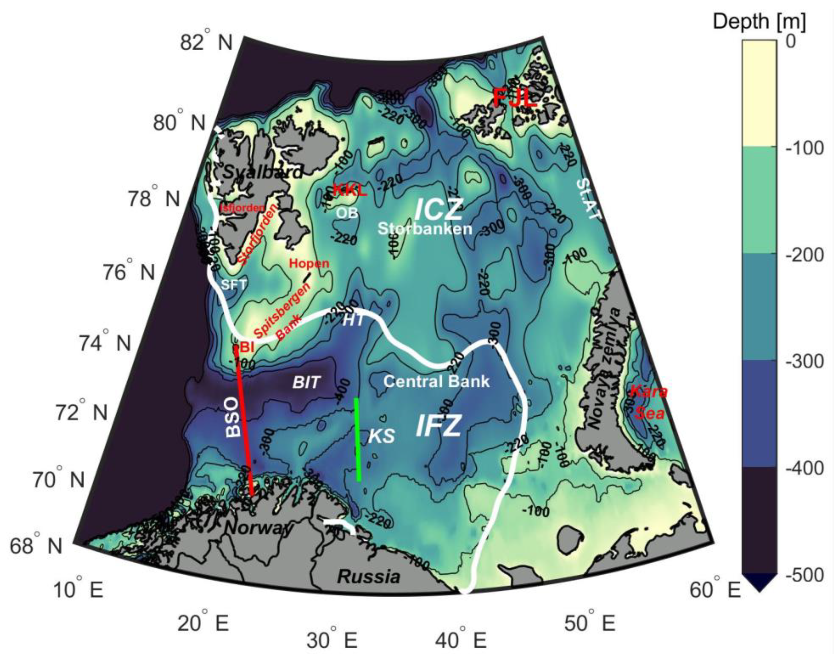
2.1. Study Area

The Barents Sea (BS) is a marginal sea of the Arctic Ocean, located between the northern coasts of Norway and Russia and three archipelagoes: Svalbard, Franz Josef Land, and Novaya Zemlya (Figure 1), and ranging over latitudes from 68 to 82°N. The mean depth of the Barents Sea is about 230 m, with a maximum depth of about 500 m (in the western part of the Bear Island Trough), while the shallowest (depth < 100 m) part is the Spitsbergen Bank (between Bear Island in the southwest and Hopen in the northeast) [50]. The Barents Sea is divided into two sub-regions in our analysis: the ice-free zone (IFZ) in the western and southern Barents Sea and the ice-covered zone (ICZ) in the eastern and northern Barents Sea. This division is based on the climatological mean of the April sea-ice edge (SIC of 15%, white line in Figure 1). In the region where the SIC is less than the 15%, the April climatological mean was masked and ignored for further temporal SIC analyses.

2.2. Datasets

Daily high-resolution (0.05° × 0.05°) optimum interpolation SST and SIC data for the Barents Sea were derived from the Operational SST and Sea Ice Analyses (OSTIA) dataset [51]. This product was created by combining data from in situ and multiple satellite sensors [Advanced Very High-Resolution Radiometer (AVHRR), Advanced Microwave Scanning Radiometer (AMSR), Tropical Rainfall Measuring Mission Microwave Imager (TMI), Advanced Along Track Scanning Radiometer (AATSR), and geostationary Spinning Enhanced Visible and Infrared Imager (SEVIRI)]. The data were obtained from the Copernicus Marine Environment Monitoring Service (CMEMS (https://resources.marine.copernicus.eu/product-detail/SST_GLO_SST_L4_REP_OBSERVATIONS_010_011/INFORMATION, last accessed: 15 February 2022)). For more details about description and data processing, see the Product User Manual and Quality Information Document that are available in the CMEMS online catalog. OSTIA data for the Barents Sea were extracted from the global data, providing a 240,033-point regularly gridded dataset spanning 14,245 days from January 1982 to December 2020.
Monthly gridded (0.25° × 0.25°) atmospheric parameters from the ERA5 dataset [52] were used to investigate the relationship between the obtained SST, SIC variability, and the local air-sea interaction. The surface air temperature at two meters altitude (SAT hereafter) and the zonal and meridional 10-m wind components (u10 and v10 hereafter) were used. The fifth generation of the European Centre for Medium-Range Weather Forecasts (ECMWF) atmospheric reanalysis data is now hosted by the Copernicus Climate Change Service Climate Data Store (https://cds.climate.copernicus.eu, last accessed: 15 February 2022). Finally, the normalized monthly mean time series of NAO and EAP climate mode indices were obtained from the NOAA Climate Prediction Centre website (https://www.cpc.ncep.noaa.gov/data/teledoc/telecontents.shtml (accessed on 30 May 2022)) in addition to the AMO index (https://psl.noaa.gov/data/timeseries/AMO/ (accessed on 30 May 2022)).

2.3. Statistical Analyses

So as to quantify the spatiotemporal variability of SST and SIC at interannual and decadal time scales over the Barents Sea (10°E–60°E, 68°N–82°N), Empirical Orthogonal Functions (EOFs) are constructed using the Singular Value Decomposition (SVD) approach [53,54]. The EOF analysis is used to extract the main modes of variability, which are composed of a spatial pattern (the so-called EOF) and a time-varying index known as the Principal Component (PC). Before performing EOF decomposition, the local mean and seasonal cycle were removed from the monthly mean time series at each grid point to obtain de-seasoned monthly anomalies of SST and SIC, which were normalized by dividing each point time series by its standard deviation to avoid points with high variability, and then the normalized anomalies were weighted by the square root of the cosine of their latitude at each grid point to account for decreasing grid sizes toward the pole [13]. Furthermore, the time series anomalies at each grid point are smoothened with a 13-month running mean filter to remove the remaining intra-seasonal variability [55]. The first and last six months of data in each time series were omitted to eliminate the edge effects of filtering. The trend is not removed before EOF analysis because the trend in the Barents Sea is related to multidecadal variability [56].
We separated the dataset into three equal periods, P1 (1982–1994), P2 (1995–2007), and P3 (2008–2020), to emphasize the sub-regional decadal variability of SST and SIC by comparing seasonal cycles, climatological mean, and cumulative trends for each period. The cumulative trend is the rate of change of SST (°C/year) or SIC (%/year) multiplied by the number of time steps for each era (13 years). The conventional least-squares approach was used to estimate the linear trends [57,58]. In order to evaluate the statistical significance of these trends at the 95% confidence interval [59], the original two-tailed Modified Mann–Kendall (MMK) test [60,61] was utilized. The MATLAB Climate Data Toolbox (M_CDT) [62] was used to compute seasonal cycles and linear trends, as well as to apply the MMK test and perform the EOF analysis.
The seasonal and monthly trends of SST and SIC were further examined to assess the intra-annual consistency of the trends throughout the year. In accordance with the general behavior of the freezing and melting cycles of sea ice in the Arctic Ocean [63], we distinguish the seasons as follows: Winter (January to March), Spring (April to June), Summer (July to September), and Autumn (October to December). The SST phenology (i.e., seasonal timing) metrics were used to assess seasonal cycle changes [64], and summer transition and duration metrics were derived from daily SST data for each year, based on the first day and the number of consecutive days that exceeded the climatological summer mean (3.6 °C), respectively. The duration of the warm summer is defined as the length of the within-year period with SSTs greater than the threshold of 3.6 °C. The duration of the sea ice season was estimated according to [10,65,66]. The average duration of the sea-ice season is calculated by counting the number of days when SIC is at least 30% for each grid point for each year and then taking the spatial average of the number of ice-covered days for the Barents Sea.
In addition, a correlation analysis was performed to quantify the role of atmospheric parameters and large-scale climate indices on the observed variability of SST and SIC. We examined the relationships between the SST and SIC and the atmospheric parameters (SAT, zonal, and meridional wind components) in the Barents Sea throughout the study period. Furthermore, the co-variability of the three selected major North Atlantic teleconnection patterns (AMO, NAO, and EAP) with the derived principal components (PCs) of the SST and SIC variations and their original time series were investigated. The statistical significance of the correlation coefficient (R) is determined using the standard two-tailed Student t-test at a 95% confidence level [67].

3. Results and Discussion

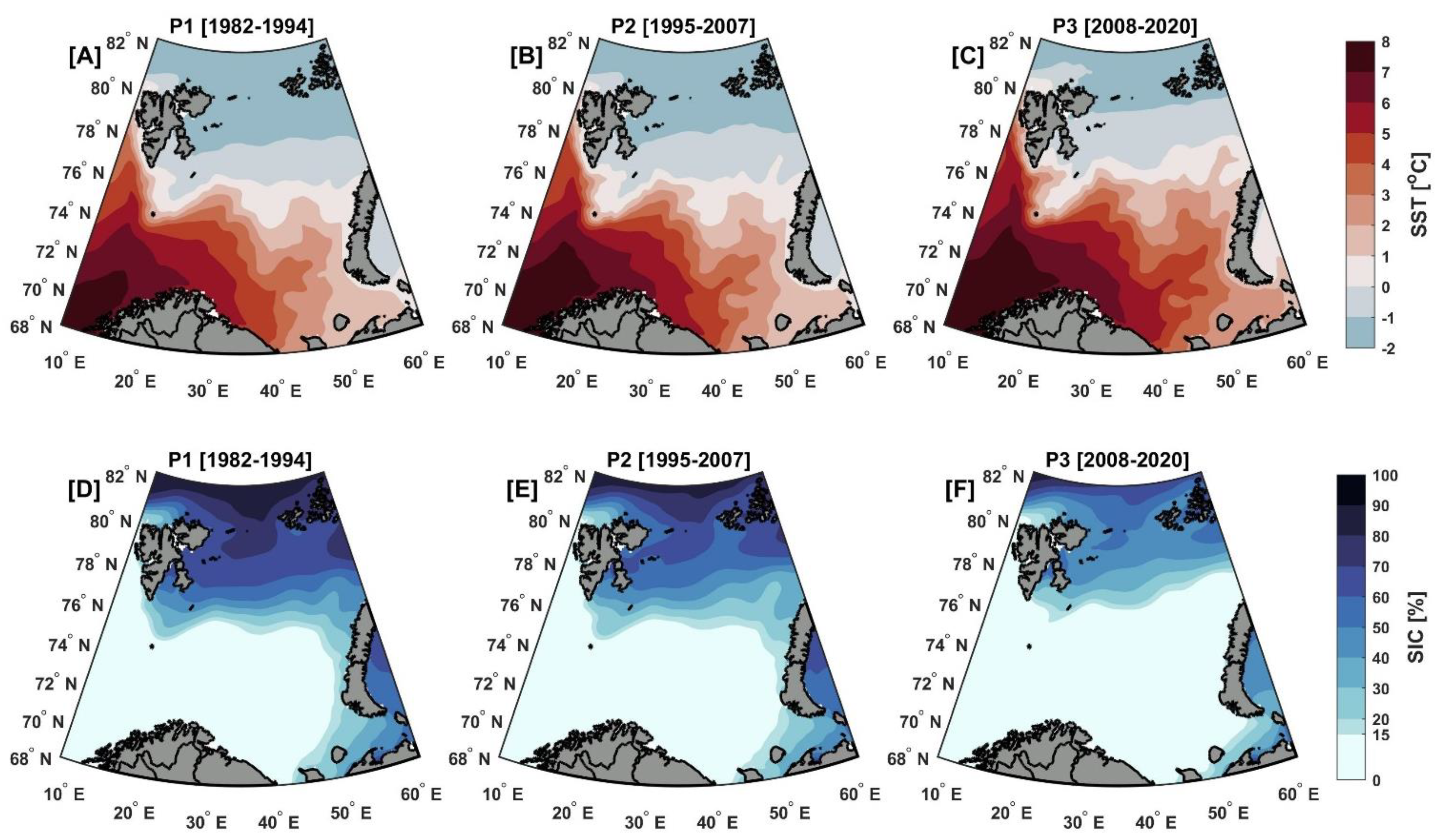
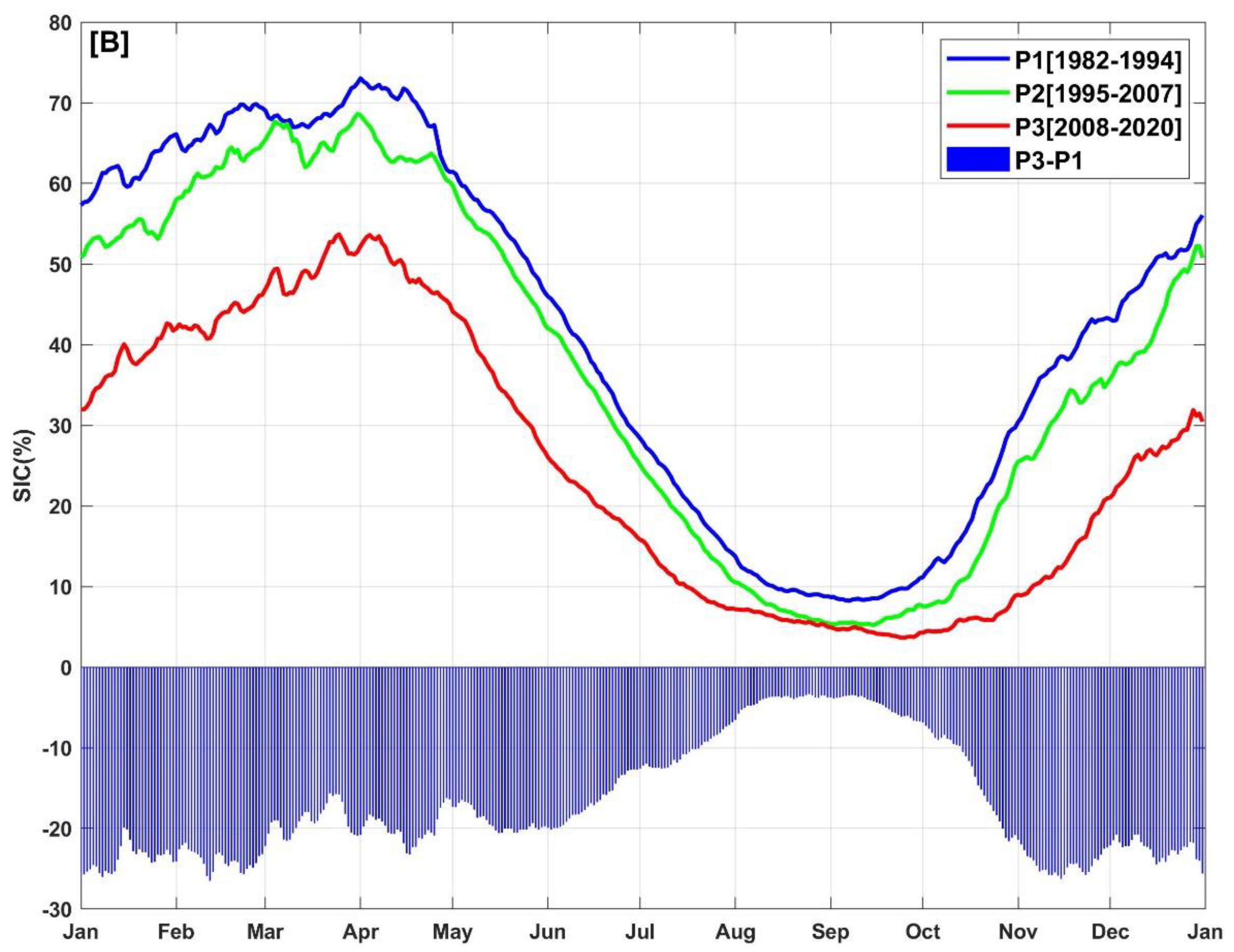
3.1. Climatology and Seasonal Cycles of SST and SIC

The temporal and spatial variability of SST and SIC in the Barents Sea was investigated using nearly four decades of satellite-derived high-resolution OSTIA data from January 1982 to December 2020. The sub-regional variability from seasonal to decadal temporal scales was analyzed by comparing the climatological mean, seasonal cycles, and cumulative trends throughout three time periods: P1 (1982–1994), P2 (1995–2007), and P3 (2008–2020). The annual SST climatology shows a general increase in SST toward the northern and eastern Barents Sea over the last period compared to the first period (Figure 2A–C), as a result of increased inflow of warm Atlantic water via the Barents Sea opening [68,69], and changes in the heat exchange between the sea and atmosphere [20], leading to sea-ice loss. In addition, anomalous southerly winds bringing warm air masses over the Barents Sea have decreased the heat loss from the ocean to the atmosphere in recent decades [20]. The average SST across the whole Barents Sea was about 1.4, 1.6, and 2.3 °C for the periods P1, P2, and P3, respectively, indicating that the regional SST climatology for the last period was higher than the first period by about 0.9 °C. As a result of these increases in SST, the open water zone (where the SIC < 15%) has typically increased toward the northern and eastern regions of the Barents Sea in comparison to the first period (Figure 2D–F). The average sea-ice area was about 0.91, 0.86, and 0.62 million km2 for the periods P1, P2, and P3, representing 48%, 45%, and 33% of the total area (1.90 million km2), respectively, indicating that the average sea-ice area has decreased by 15% between the first and last periods. The climatological annual, winter, and summer averages for SST and SIC over the entire study period are shown in Figure S1A–F. These figures show that, in summer, the Barents Sea is almost ice-free (i.e., SIC < 15), and AW covers a large part of the Barents Sea, while in winter, the cold Arctic water occupies a large part of the northern Barents Sea and the Kara Sea, with SIC exceeding 80% (Figure S1B,E).
Figure 3 depicts the daily climatological mean of SST and SIC and their seasonal cycles calculated for the periods P1, P2, and P3, as well as the daily SST/SIC increases/decreases between the last and first periods (P3-P1) in absolute values. In general, the daily seasonal cycle analysis revealed that the highest SST value was in August and the lowest in March/April, while the SIC reaches its maximum values in March/April and minimum in August/September. These findings are consistent with previous studies [70,71]. The amplitude of the daily mean SST seasonal variability over the three periods was found to be about 5 °C. The SST seasonal cycle confirms the recent warm transition in the Barents Sea, as the SST gradually increases from P1 to P3. In the first period, P1, the 3.6 °C average was only surpassed in the summer months (July, August, and September), whereas in the last period, P3, this occurred in four months (July, August, September, and October), with monthly temperatures close to 7 °C reported in August 2013 and 2016. According to these findings, the warm season began earlier, was more intense, and lasted longer, with average SST increases of up to 1 °C through October and November between P1 and P3 (Figure 3A, red bars). The lowest SST increase (~0.55 °C) between the two periods was found in March and April. The greatest decrease/difference of sea ice between the two periods occurred during the winter rather than the summer, which was consistent with the findings of [70], with an average daily SIC decrease of −22% from November through April and of −11% from May through October over P3 compared to P1 (Figure 3B, blue bars). This indicates that the value of sea ice loss during winter is double that of the summer. The mean annual SST and SIC difference between P3 and P1 are 0.83 °C and −17%, respectively.

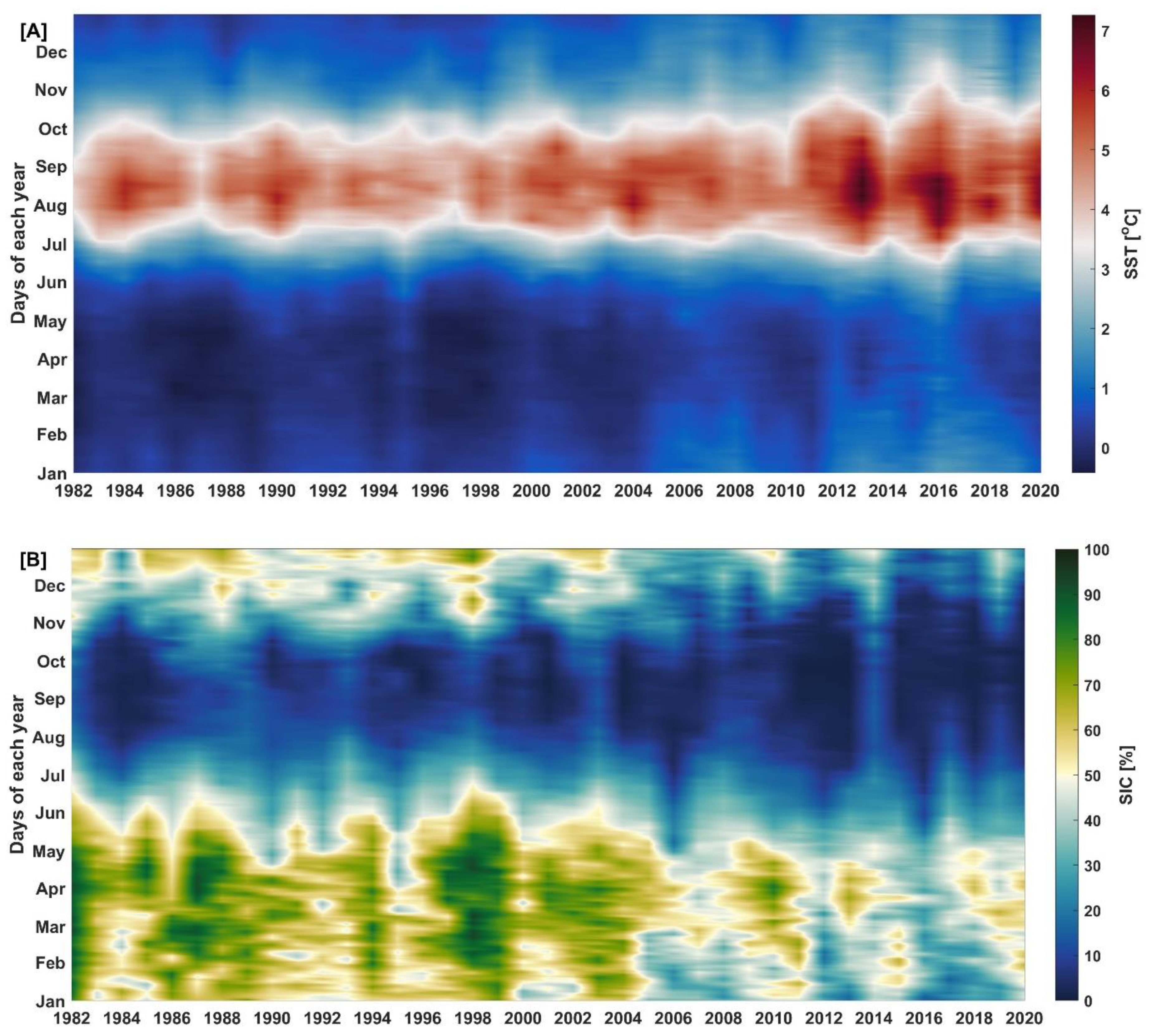
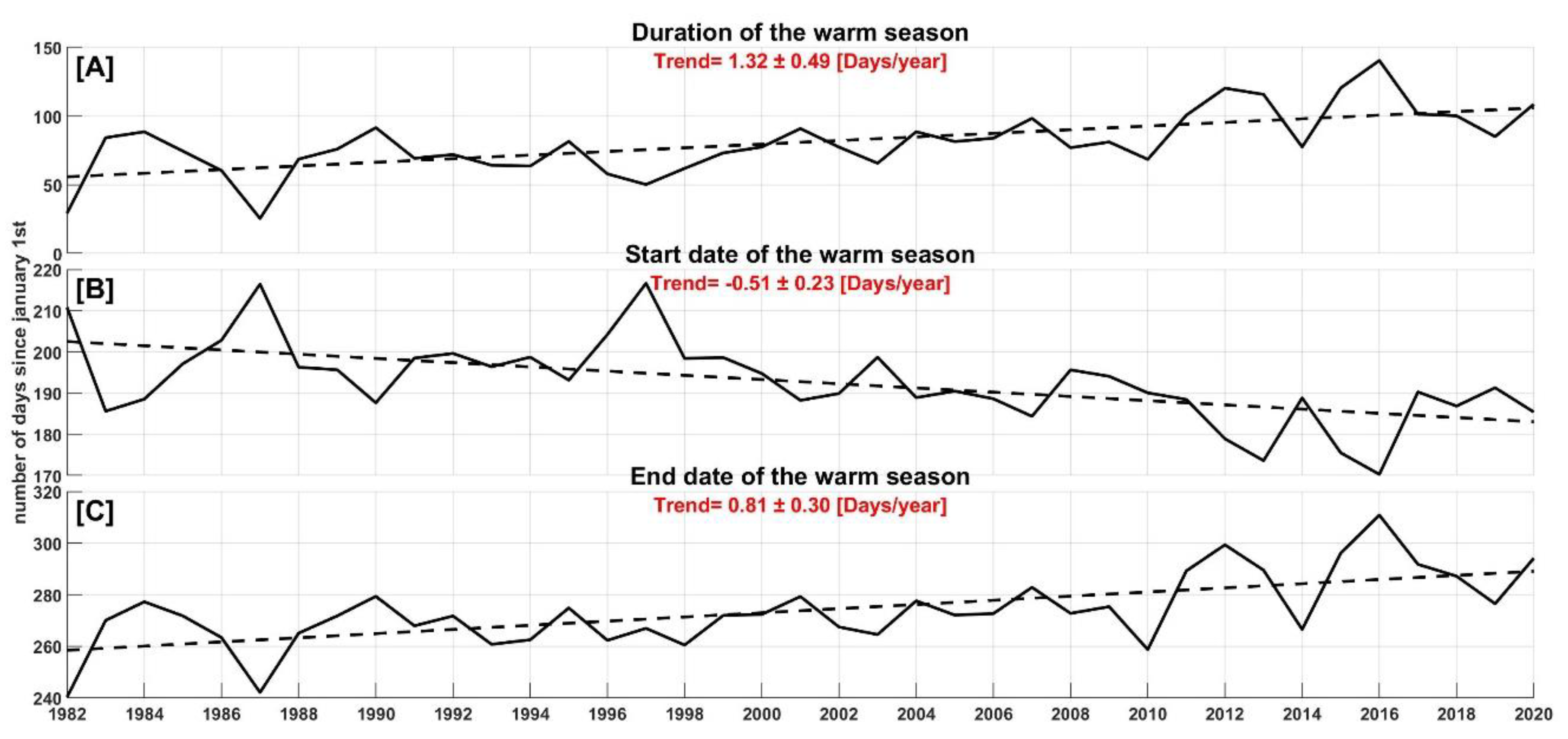
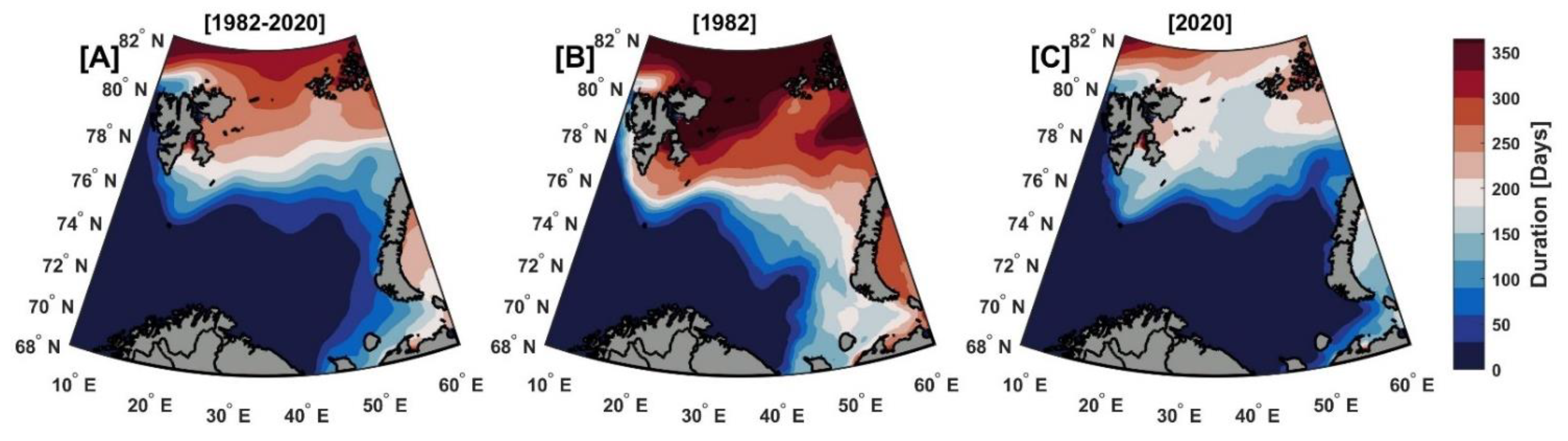
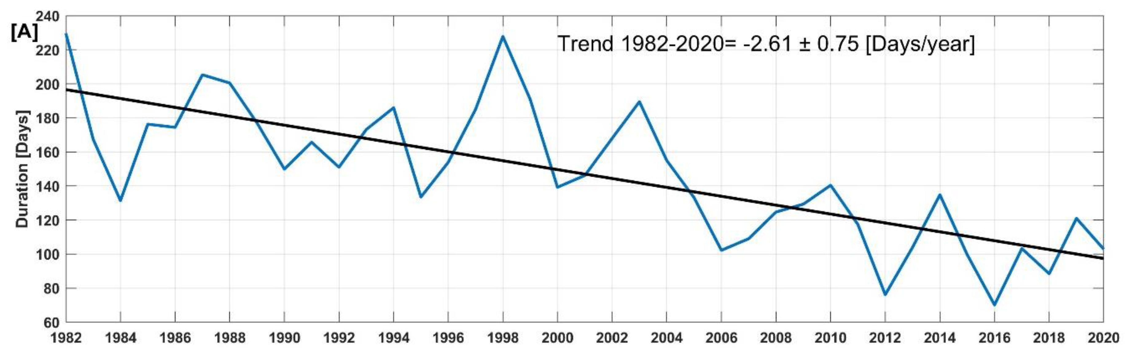
3.2. Phenology of SST and Sea-Ice Cover Duration

The global means of the SST and SIC time series have been built by averaging daily data from all grid points inside the Barents Sea throughout the analyzed period from 1982 through 2020 and plotted using a Hovmöller diagram (daily vs. annual) as seen in Figure 4. The overall SST increase was dominated by significant increases during the warm seasons (Figure 4A), which resulted in sea-ice thinning and large areas becoming ice-free during the summer melt season (Figure 4B). The rise in SST during warm seasons also causes phenology shifts in the seasonal cycle (Figure 5). Summer transition and duration metrics revealed significant trends toward earlier summer onsets (−0.51 ± 0.23 days/year), and later summer ends (+0.81 ± 0.30 days/year) resulting in an extended duration of 51.48 ± 18.62 warm summer days (+1.32 ± 0.49 days/year) over the entire 39-year period (1982–2020).
Analysis of average annual sea-ice duration has revealed patterns of change and trends in sea-ice season duration from 1982 through 2020 (Figure 6 and Figure 7). The average duration of the sea-ice season during the P1, P2, and P3 periods was 175, 156, and 108 days, respectively. Over the entire study period (1982–2020), the Barents Sea was covered with sea ice for 147 days per year (~5 months per year). The most severe and longest winters during the study period occurred in 1982 and 1998, resulting in ice formation over most of the Barents Sea, with sea-ice season durations of about 230 days and 228 days, respectively (i.e., >7.6 months). The lowest ice duration (<70 days) was observed in 2016 (Figure 7A), the warmest year of the entire study period (see Figure 8D,E). In general, the average annual duration of the sea-ice season in the Barents Sea decreases southward (Figure 6A), and there is a marked difference in the sea-ice conditions between the beginning (1982) and the end (2020) of the study period, including a reduction in permanent ice cover zone (duration > 360 days) in the northern Barents Sea and a shift of large areas in the southern Barents Sea from ice-cover zone to ice-free zone (Figure 6A–C).
The duration of the sea-ice season decreases at a rate of −2.61 ± 0.75 days/year (Figure 7A), resulting in a 3.4-month shorter/longer sea-ice/sea-ice-free season duration over the last 39 years. This rate is very high compared to the rate observed by [10,12] over the entire Arctic region during the period (1979–2013) and (1980–2015), respectively. They found that the rate of the sea-ice season duration was about −0.5 days/year and −0.98 days/year, respectively. A statistically significant (p < 0.05) negative trend in the duration of sea-ice season was observed over the entire Barents Sea from 1982 through 2020 (Figure 7B). This implies that the sea-ice seasons in the Barents Sea are becoming shorter, and we can expect that a continued warming climate will lead to a further lengthening of the ice-free season. The most negative trends in sea-ice season duration (reaching −6 days/year) are observed in the northeastern Barents Sea (mainly between FJL and Novaya Zemlya; Figure 7B). The trend pattern in sea-ice season duration (Figure 7B) is similar to the trend of SIC (Figure 8D), suggesting that SIC is lower on average when sea-ice duration is shorter and vice versa when it is higher SIC.

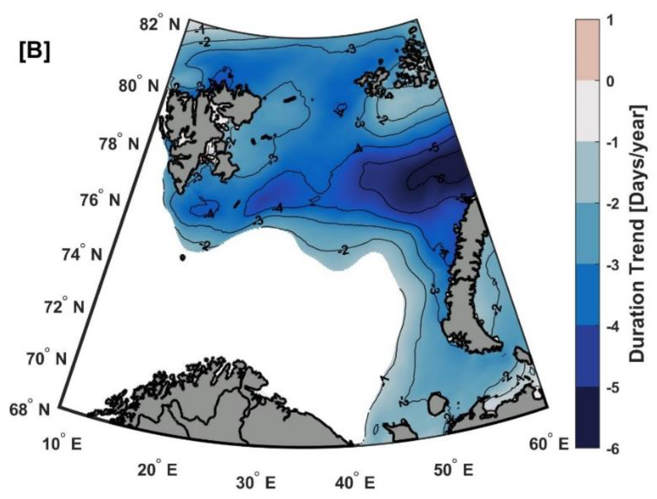
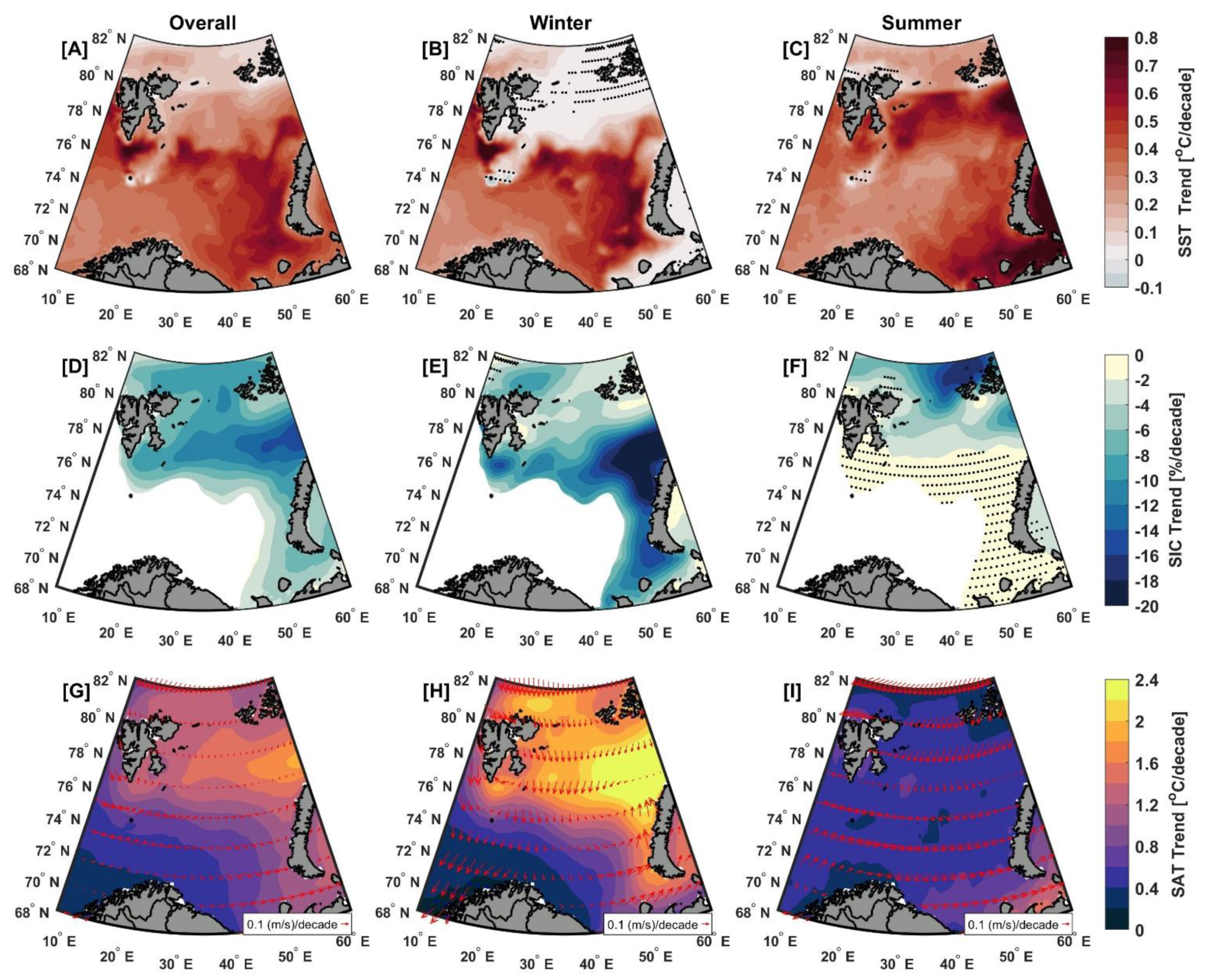
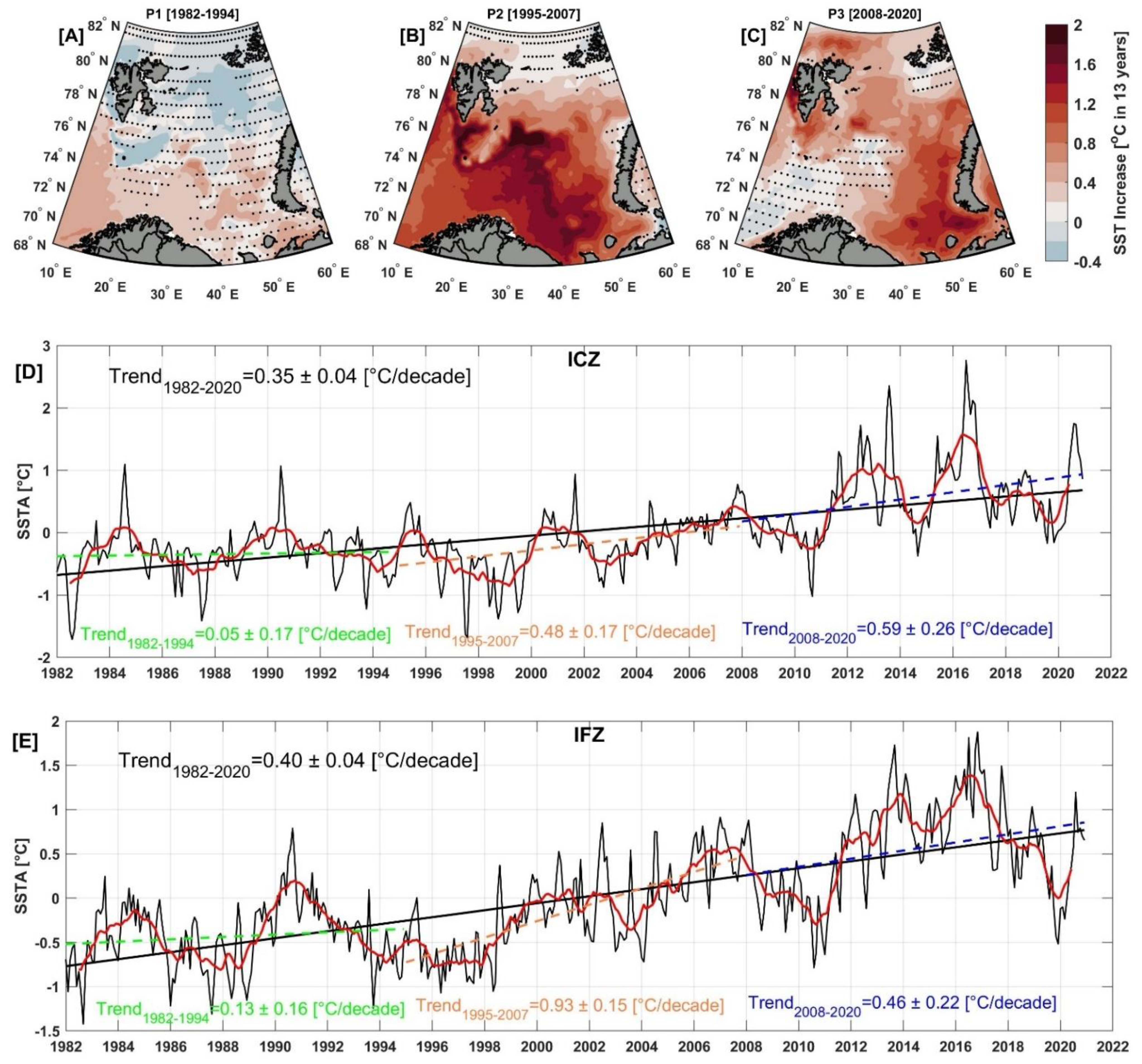
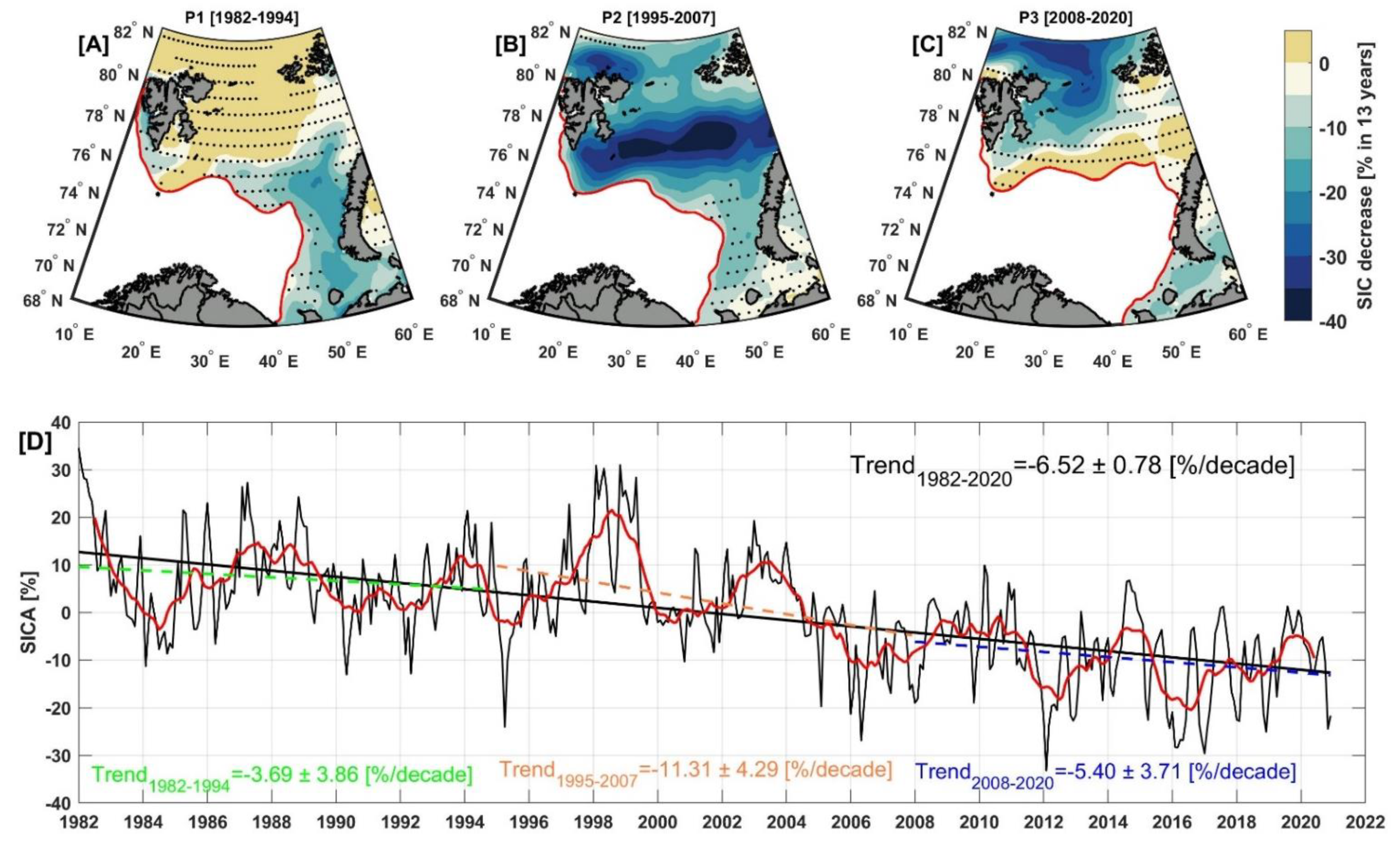
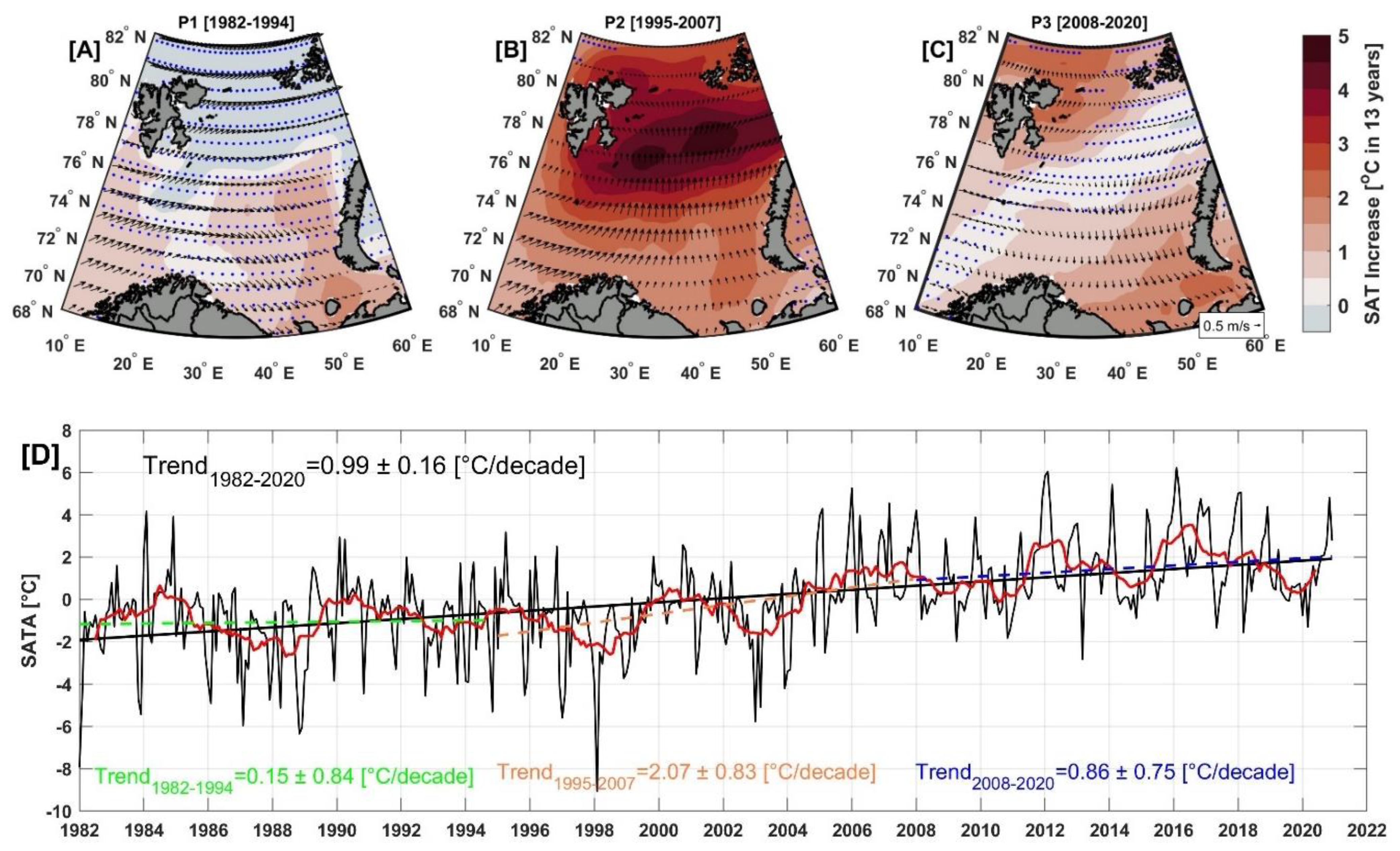
3.3. Spatio-Temporal Trends in Ocean and Atmosphere Warming and SIC Reduction

The spatial and temporal trend patterns of de-seasonal SST, SIC, and SAT in the Barents Sea from 1982 to 2020 are shown in Figure 8A,D,G, Figure 9D,E, Figure 10D and Figure 11D, respectively, along with the cumulative spatial trends for each period P1, P2, and P3. According to the MMK test [60], the spatial distribution of these trend patterns is statistically significant for both oceanic and atmospheric warming and sea-ice retreat throughout the Barents Sea (Figure 8A,D,G). The overall regionally averaged warming trend of SST was about 0.35 ± 0.04 and 0.40 ± 0.04 °C/decade over the ice-covered and ice-free zones (Figure 9D,E), respectively. This SST warming rate was associated with a SIC decrease of −6.52 ± 0.78%/decade (Figure 10D) and atmospheric warming of about 0.99 ± 0.16 °C/decade over the entire Barents Sea (Figure 11D). The decline of SIC is consistent with [63], which found that the rate of decline of SIC was about −5.4%/decade during 1979–2016. The highest SST anomaly value was recorded over the entire Barents Sea (i.e., over both ICZ and IFZ) in the summers of 2013 and 2016 (Figure 9D,E), while the lowest value was reported over the entire Barents Sea in the winter of 1982 (Figure 9D,E). The maximum SIC values were observed in 1982 and 1998 (Figure 10D). The 13-month running mean of SST anomaly values (red lines in Figure 9D,E) further indicate the interannual/decadal SST variation from 1982 through 2020. The Barents Sea SST varied weakly from 1982 to 1998, followed by strong variations from 1998 to 2011 and then an even stronger oscillation from 2011 through 2020.
Moreover, seasonal and monthly trend analyses of SST and SIC were carried out to examine the consistency of intra-annual trends over the entire period (Figure 8 and Figure S2). The spatial average of the SST trend in summer was significantly higher (0.38 ± 0.11 °C/decade) than the SST trend in winter (0.25 ± 0.05 °C/decade). SST warming trends in summer were not only higher but also showed different spatial patterns (Figure 8C) than in winter (Figure 8B), suggesting that the Barents Sea exhibits considerable time-dependent spatial variability. The highest SST trend was observed in summer over most of the Barents Sea, including the northern and central parts (Figure 8C), while in winter, it was only observed in the southern part (mainly below the April ice edge), as this region was dominated by increasingly warmer Atlantic water for most of the year. Monthly and seasonal changes in the SIC followed the fluctuations of warm Atlantic waters [15,50]. Significant spatial variability in SIC trend patterns is found between winter and summer (Figure 8E,F). A strong negative SIC trend was observed in winter (−8.15 ± 2.40%/decade) and less in summer (−4.00 ± 1.96%/decade). During winter, the strongest negative trend in sea ice was observed in the northern and western regions of the Novaya Zemlya (Figure 8E), in conjunction with southerly wind patterns along the Novaya Zemlya (red arrows in Figure 8H), which enhanced surface currents and AW heat flux to the north and amplified atmospheric warming north of the Novaya Zemlya (yellow shaded region in Figure 8H). During summer, the lowest SIC was observed in the northeastern part of the Barents Sea (Figure 8F), reflecting warmer Atlantic waters that moved farther north (Figure 8C). Northerly wind patterns (red arrows in Figure 8I) also contributed to lower surface air temperature (shading in Figure 8I), greater heat loss and increased sea-ice transport from the Arctic Ocean into the Barents Sea [46]. Monthly trend analysis (Figure S2) indicates that the lowest SST warming rate is found from February through May, with values below the annually averaged trend (0.33 ± 0.08 °C/decade). The largest warming rate appears from July through November (Figure S2A). The sea-ice loss occurs in all months, with the highest negative trends in November–February, and the smallest declines in August and September. The rate of ice reduction is almost constant from March through June (Figure S2B), with values very close to the annually averaged trend (−6.52 ± 1.89%/decade). From this analysis, it is evident that ice loss is greater in winter than in summer.
The warming and ice-reduction trends are not consistent in space and time throughout different historical periods (Figure 9 and Figure 10). For the cold P1 period (1982–1994), both SST and SIC showed non-statistically significant (p > 0.05) trends at spatial (Figure 9A and Figure 10A) and temporal (Figure 9D,E and Figure 10D) scales. During the P2 period (1995–2007), the Barents Sea warmed dramatically and transitioned to a warmer state (Figure 9B), with a sharp decrease in the SIC trend (Figure 10B), due to the increased inflow of warmer Atlantic water that spread further east- and poleward during this period [68]. The average SST warming trend was about 0.48 ± 0.17 and 0.93 ± 0.15 °C/decade over the ice-covered and ice-free zones, respectively (Figure 9D,E). The SST trend shows a high spatial variability over the Barents Sea. The strongest SST warming trends occurred in the open water region (i.e., IFZ), with a total increase of SST reaching 2 °C over this 13-year period (Figure 9B) in southern Svalbard (Storfjorden Trough), the Hopen Trough, and the Central Bank (see locations in Figure 1). These results are consistent with the results of Asbjørnsen et al. (2020) [68], who found that the largest SST warming trends occurred south of the winter ice edge, with increased ocean heat advection and reduced surface heat loss acting as the main drivers. The spatial average of the sea-ice decline was exceptionally high (−11.31 ± 4.29%/decade) during P2 (Figure 10D), reflecting the accelerated SST warming trend during this period (Figure 9E). The most negative and significant cumulative SIC trend (up to −40%) was observed in the central Barents Sea between Novaya Zemlya, Svalbard, and Franz Josef Land (Figure 10B). A sharp decline in SIC was also found north and northeast of Svalbard (Figure 10B), owing to the existence of a sensible heat polynya (i.e., an area of open water surrounded by ice) in this region known as Whalers Bay [72]. A quasi-steady re-opening and eastward progression of this sensible heat polynya were observed in this area as a result of the intrusion of the warm Atlantic Water (AW) carried by the West Spitsbergen Current [13] from the Nordic Seas [73,74].
Over the P3 period (2008–2020), the ice-free zone was characterized by a much lower SST trend (0.40 ± 0.04 °C/decade) compared to the P2 period trend (0.93 ± 0.15 °C/decade) (Figure 9E). The high SST trends during P3 shifted east- and northward (Figure 9C), resulting in an average warming rate of about 0.59 ± 0.26 °C/decade over the ice-covered zone (Figure 9D). The highest SST trend was observed over the eastern part of the Barents Sea, with a cumulative trend exceeding 1.2 °C in the southeastern Barents Sea. The northern Barents Sea showed relatively small trends during P3 but still significant (p < 0.05) over most of the region. A non-significant warming trend was observed only in the southwestern Barents Sea and south of Franz Josef Land during P3. The high SST trends in the eastern Barents Sea are caused by a rise in Atlantic Water temperatures in the Kola Section [56]. The spatial average of sea-ice reduction during P3 was about −5.40 ± 3.71%/decade. The sensible heat polynya was primarily located in the north and northeast of Svalbard during P2 (1995–2007) but extended further east to 50°E during P3 (2008–2020). As a result, the largest negative cumulative trend of sea ice (up to −35%) was observed in the north region (between Svalbard and FJL) during P3 (Figure 10C). A non-significant increase in the SIC trend is observed over the central and northeastern Barents Sea in association with a northeasterly wind trend between FJL and Novaya Zemlya (Figure 11C). This suggests that more sea ice is flowing into the northeastern Barents Sea between FJL and Novaya Zemlya during this period [25].
Figure 11A–C shows the cumulative spatial trends of the surface air temperatures and wind vector anomalies for each period P1, P2, and P3. The spatial pattern and significance of atmospheric warming during the various subperiods are consistent with that of SIC (Figure 10A–C). For the cold P1 period (1982–1994), air temperature showed non-statistically significant (p > 0.05) trends at spatial (Figure 11A) and temporal (Figure 11D) scales, except in the southeastern part of the Barents Sea, which was associated with the northwesterly wind trend. During the P2 period (1995–2007), amplified significant atmospheric warming was observed over the entire Barents Sea, with a spatially average SAT trend of about 2.07 ± 0.83 °C/decade (Figure 11D). The highest cumulative SAT trend during this period was observed in the central Barents Sea between Novaya Zemlya, Svalbard, and Franz Josef Land (i.e., the same region that has the lowest SIC trend), with an overall increase of SAT of up to 5 °C during this 13-year period (Figure 11B). This atmospheric warming was accompanied by a southwesterly wind trend in the southwestern region and a southerly wind trend over most of the Barents Sea (arrows in Figure 11B). The southwesterly wind at the BSO induces Ekman transport and enhances the inflow of warm AW into the Barents Sea [75], and in addition, the southerly wind over most of the region enhances the advection of warm air masses from the south into the northern Barents Sea [20], resulting in a sharp decrease in SIC during this period (Figure 10B). During the P3 period (2008–2020), atmospheric warming was about 0.86 ± 0.85 °C/decade (Figure 11D), which is lower than the warming observed during the P2 period. The highest significant SAT trends are observed in the north and east of Svalbard and in the southeastern region of the Barents Sea (Figure 11C), while non-significant trends (p > 0.05) are observed in the central and southwestern regions (i.e., the Barents Sea opening). During this period, a divergence pattern of the wind vector trends is observed, with a south wind trend in the north and east of Svalbard and a northwest wind trend in the southeast region of the Barents Sea (black arrows in Figure 11C). The suppressing of the southwesterly wind trend at the Barents Sea opening could be an indicator of a reduced inflow of warm AW into the Barents Sea and an increase in the outflow of fresh and cold water from the Barents Sea. In general, these results suggest that in addition to the role of warm AW inflow into the Barents Sea, which has been well documented in several previous studies [16,20,25,75], atmospheric forcing most likely plays an important role in the reduction of SIC in the Barents Sea. Especially during the warm P2 period. The sea-ice condition in the Barents Sea is mainly determined by atmospheric circulation, either directly (i.e., meridional north–south winds redistributing sea ice and bringing warm air masses over the Barents Sea) or indirectly (i.e., increase/decrease of inflow of AW into the Barents Sea). In the following section, we will discuss in more detail the correlation between SST/SIC and atmospheric parameters.

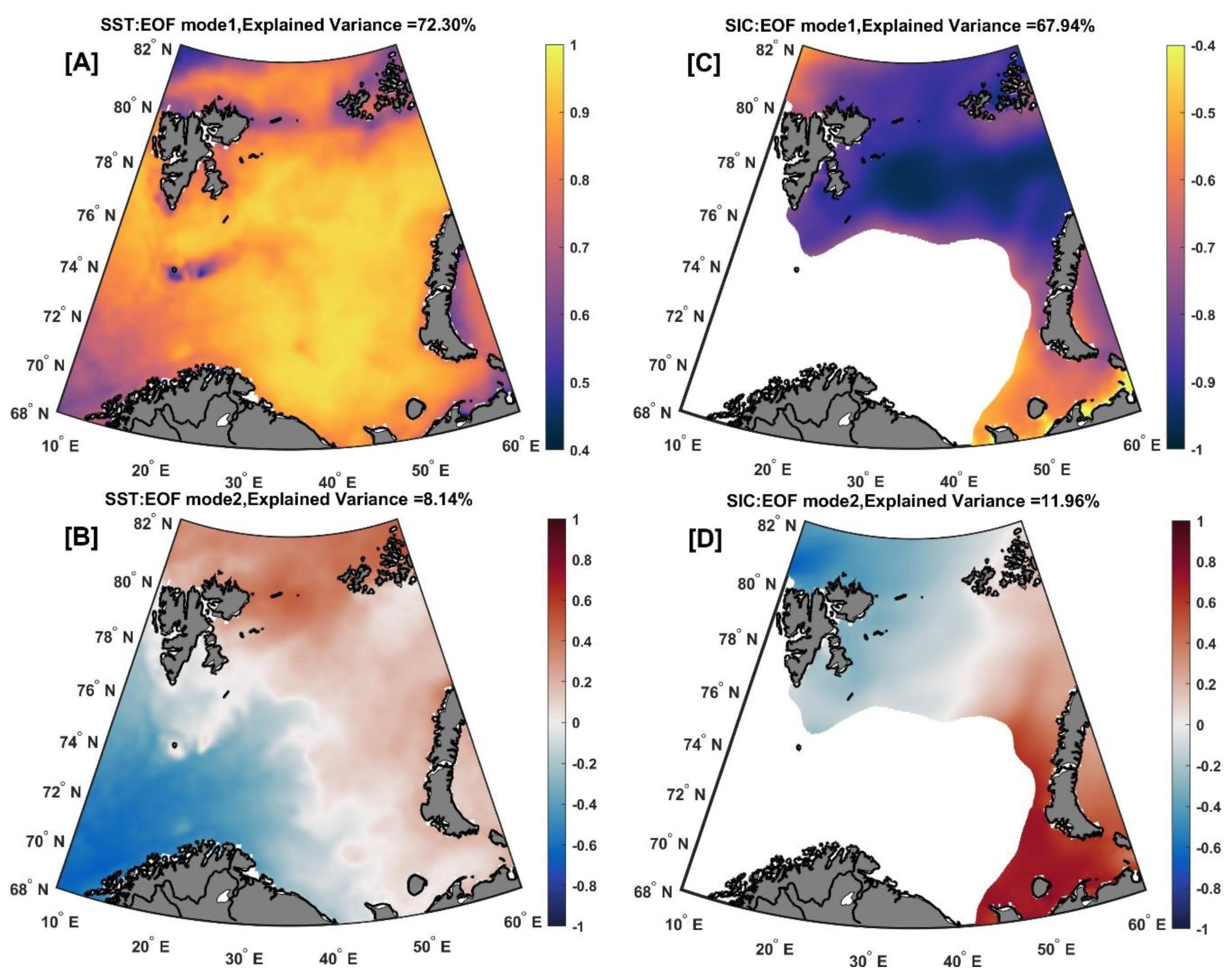
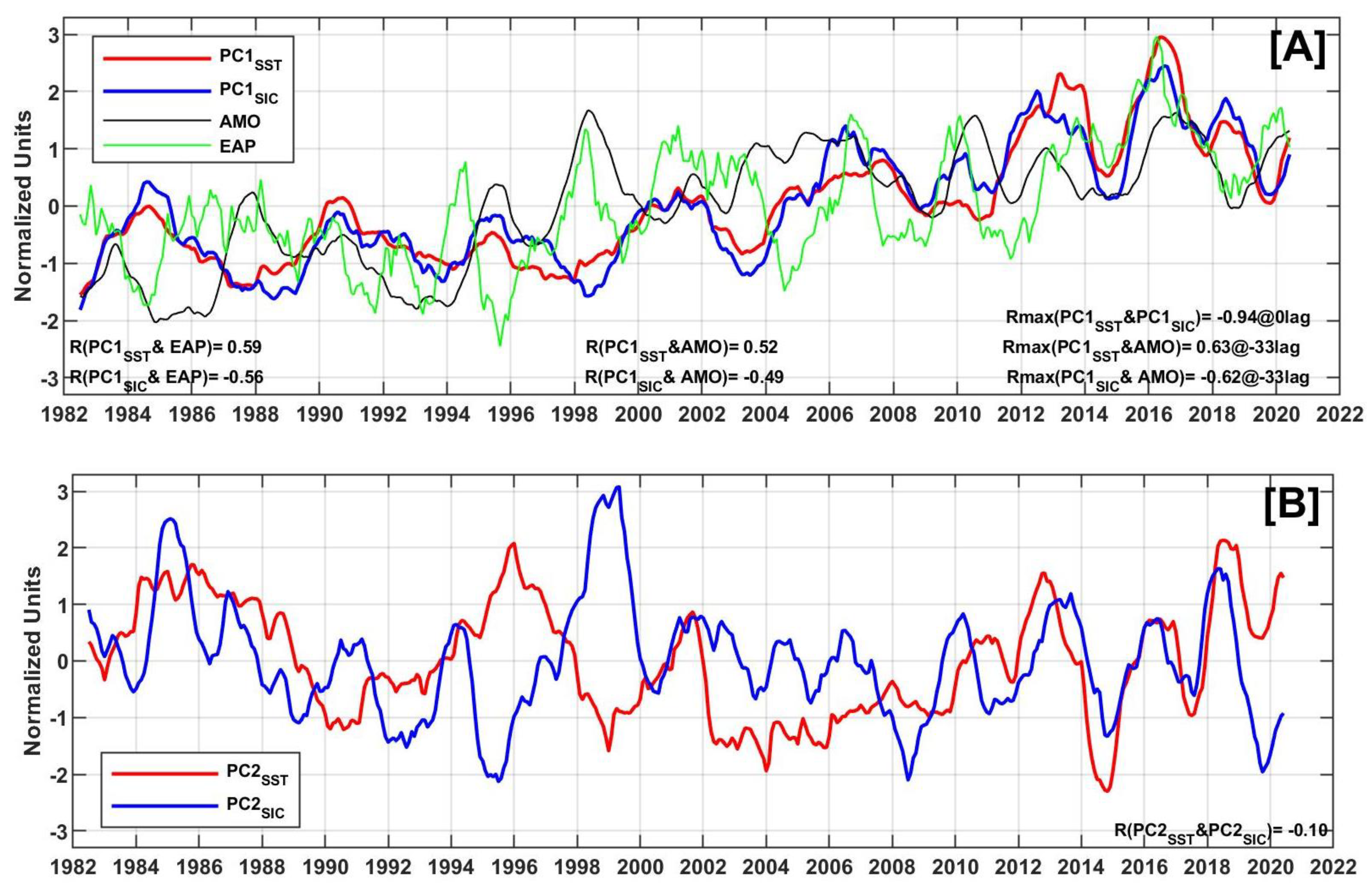
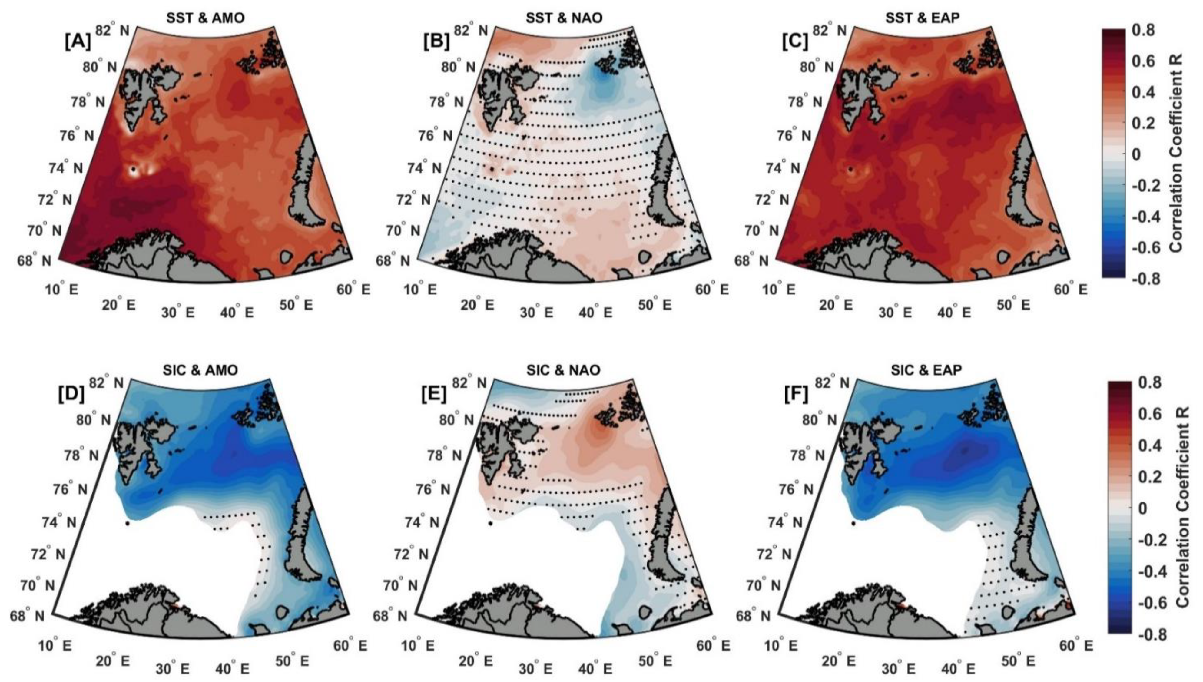
3.4. Interannual Variability of SST and SIC and Their Relation to Large-Scale Teleconnection Patterns

The authors calculated the percentage of variance represented by the stationary seasonal cycle and the de-seasoned signal to quantify the interannual variability of SST and SIC, as described in [76,77]. This is achieved by calculating the spatially average of temporal variances at each grid point for both original (observed) data sets representing the total variability (seasonal and non-seasonal signal) and residual data sets simply representing the de-seasoned and de-trended signal. We found that the interannual SST variability accounts for 6.5% of the total SST variability in the Barents Sea as a spatial mean, ranging from 2.5% (in the southwestern region) to 30% (in the northwestern region of the study area), and higher interannual SST variability was also found over the polar front region (see Figure S3A). The corresponding average interannual variability of SIC accounts for 13% of the total variability of SIC and ranges from 0 (south of FJL and over the Kara Sea) to 35% (over the sea-ice edge region) (see Figure S3B). In general, the higher interannual variability of SST and SIC is associated with the position of the polar front and follows the propagation/influence area of AW. The lower interannual variability over most of the Barents Sea suggests that SST and SIC exhibit very high seasonal variability.
The spatially coherent interannual variability of SST and SIC are evaluated by using EOFs. The first two EOF modes account for 80% and 79% of the total non-seasonal variance in SST and SIC, respectively. Here, we only discuss the first two EOF modes because the third mode explains less than 5% of the variance in both SST and SIC. The SST EOF1 mode accounts for 72% of the total non-seasonal variance and captures interannual and decadal SST variability. The spatial distribution pattern of this mode displays a positive anomaly across the whole Barents Sea (Figure 12A), indicating that the entire basin is oscillating in-phase around the steady-state mean. In-phase heating or cooling implies a decrease or increase in the concentration of sea ice throughout the Barents Sea. The highest SST variability was observed over the shallow bank area between Hopen and Bear Island (Spitsbergen Banken, see Figure 1) and over the central and southeastern Barents Sea (mainly in the region between the northern and southern Polar Front, as defined by Oziel et al., (2016) [40] in their Figure 5), which is affected by both warm Atlantic Water from the south and cold Arctic Water from the north. The lowest SST variability was found in the southwestern, northwestern, and northeastern Barents Sea. This low variability in the de-seasoned time series is due to the southwest region being affected only by warm Atlantic Water, whereas the northwest and northeast regions are affected mainly by cold Arctic Water. The spatial distribution pattern of the SST EOF2 mode (Figure 12B), which explains about 8% of the total de-seasoned variance, exhibits a dipole (out-of-phase) oscillation, with opposite variations between the ice-covered zone (ICZ) and the ice-free zone (IFZ) (i.e., positive anomalies over the ICZ and negative anomalies over the IFZ). The maximum variability was found in the northeastern Barents Sea, while the opposite maximum variability was found in the southwestern Barents Sea.
The spatial pattern of the SIC EOF1 mode explains about 68% of the total variance in the de-seasoned interannual SIC and shows a negative anomaly over the whole Barents Sea (Figure 12C), indicating an in-phase decrease in SIC over the entire Barents Sea between 1982 and 2020. The most negative variability (center of the action) was found over Storbanken and Olga Basin (see Figure 1 for location) and in the northeastern Barents Sea. The SIC EOF2 mode (explains about 12%) shows a dipolar structure, with negative sea ice anomaly around and east of Svalbard and positive anomaly around Novaya Zemlya and south and east of Frans Josef Land (Figure 12D). The magnitude of SIC anomalies associated with this mode is generally less than that of SIC EOF1, except in the south of the Novaya Zemlya region, which is largely influenced by the AW inflow. This dipolar structure of the SIC EOF2 is consistent with [25].
The corresponding temporal coefficients PC1SST and PC1SIC of the first EOF mode (Figure 13A) show a general increase/decrease in SST/SIC (note that for SIC, the upward trend of PC1SIC corresponds to the decrease of sea ice (negative SIC anomalies), as we draw the inverted SIC PCs for better visualization). This mode captures the interannual and decadal variability of SST and SIC, with a pronounced alternation of positive and negative peaks on an interannual time scale with a period of 5–6 years. The highest peaks (warm periods, low SIC) were observed in 1984, 1990, 2006, 2012/2013, and 2016. The most prominent and isolated peaks found in PC1SST were associated with the occurrences of the Barents Sea marine heatwaves [19]. The signatures of the most intense marine heatwaves that occurred in 2013 and 2016 [19] were clearly visible in the Barents Sea ICZ and IFZ (Figure 9D,E). The highest peak was observed in 2016, the warmest year on record, which coincided with the strongest positive phase of EAP [19]. The lowest peaks (cold periods, high SIC) were recorded in 1982, 1987/1988, 1997/1998, 2003, 2011, 2014, and 2019. The strong significant correlation coefficient (R = −0.85) between PC1SST and PC1SIC indicates that both the SST and SIC exhibit strong coherent co-variability on the interannual time scale (Figure 13A). The temporal coefficients of the second EOF modes PC2SST and PC2SIC show considerable variability on both the high-frequency and interannual/decadal scales (Figure 13B). During the last period, P3 (2008–2020), PC2SST and PC2 SIC coincide on the interannual scale, while during the first two periods, they fluctuate in opposite directions on the multiyear scale. However, there is no significant relationship between them over the whole study period (R = −0.1, see Figure 13B). The highest peak of PC2SIC in 1998/1999 coincides with a strong positive phase of both AMO and EAP, while the lowest peak in 1995 is associated with the strongest negative phase of EAP.
We examine the frequency distribution of SST and SIC variability in the Barents Sea based on the power spectral density of the filtered (13-month running mean) and detrended time series of the SST and SIC using the Welch method [78]. Spectra are plotted on a logarithmic scale to highlight a wider range of variability (Figure S6). After removing the seasonal variability by the running mean, the variability can be divided into three frequency ranges consisting of the interannual, the decadal, and the multidecadal cycle. Both SST and SIC show a strong peak on the interannual time scale between 5–6 years, centered at about 5.4 years (Figure S6A,B). This result is consistent with [43], who found the same peak in the simulated AW temperature at the BSO. The second peak is found with a periodicity of 10.7 years for both SST and SIC but is less pronounced for SIC. The same results are obtained for the first principal component of SST and SIC, indicating that the first EOF mode is a combination of interannual and decadal variability. These density spectra are in good agreement with the SSTA and SICA observations in Figure 9 and Figure 10. Therefore, we used the 6-year running mean to remove interannual variability and then examined the relationship between SST, SIC, and their principal components with different climate modes at the decadal scale.
The large-scale variability of atmospheric circulation can be characterized by teleconnection patterns, where circulation anomalies are interconnected over large distances. Regional climate patterns cannot be understood without considering the effects of large-scale atmospheric circulation variability [79]. In order to investigate the effects of different teleconnection patterns on the SST and SIC in the Barents Sea, the normalized time series of the AMO, NAO, and EAP were used for correlation analyses with the spatially averaged SST and SIC time series and their EOF principal components. On the interannual time scale (i.e., 13-month running mean), the AMO index showed significant correlations with the PC1SST (R = 0.52) and PC1SIC (R = −0.49) (Figure 13A). Further analysis of the lead-lag correlation revealed a lag of 30–37 months (~3 years), in which the AMO index was found to lead the first principal component of both the SST and SIC (Figure 13A and Figure S4). This correlation highlights the link between SST and SIC variability in the Barents Sea with the SST oscillation in the North Atlantic and, thus, the role of AW inflow into the Barents Sea. Particularly, on the decadal time scale (i.e., 6-year running mean), the AMO index showed a remarkably high correlation with the PC1 of the SST and SIC, with values of 0.75 and −0.76, respectively (Table 1 and Figure S5A,B).
The EAP index also showed significant correlations with the PC1SST (R = 0.59) and the PC1SIC (R = −0.56) on the interannual time scale (Figure 13A), without showing significant lags. On the decadal scale, a higher correlation was observed between the EAP and the PC1 of SST (R = 0.90) and SIC (R = −0.87) (see Table 1 and Figure S5A,B). No statistically significant correlations were found for the NAO index on annual and interannual time scales, either with the SST/SIC time series or with their principal components (Table 1). The second modes of SST and SIC were not correlated with any of the selected large-scale atmospheric variability patterns on different time scales (Table 1). However, there seems to be a connection between the NAO and the decadal variations of SST (R = 0.45), which is especially evident in the second EOF mode of SST anomalies (Table 1 and Figure S5C).
In addition, Figure 14 shows the spatial distribution of correlation coefficients between the interannual variability of SST, SIC, and the selected climate indices (AMO, NAO, and EAP). The AMO index shows a higher significant positive and negative correlation over the entire Barents Sea with SST and SIC, respectively (Figure 14A,D). The highest positive correlation between SST and AMO is found over the open water region (Figure 14A), which is directly influenced by the AW inflow. The highest negative correlation between SIC and AMO is observed over the region with a stronger negative SIC trend (i.e., the SIC trend and the correlation between SIC variability and AMO show similar patterns) (see Figure 8D and Figure 14D). Although the NAO index is not significantly correlated with SST and SIC on different time scales (Table 1), the spatial correlation between SST and NAO (Figure 14B) shows a significant positive relationship between them over the Kola section and north of Svalbard and a negative correlation south of Frans Josef-Land, and vice versa with SIC (Figure 14E). EAP shows a highly significant positive correlation with SST over the entire Barents Sea (Figure 14C), while this correlation with SIC is negative over most of the Barents Sea, except for the southeastern part, which shows a nonsignificant correlation (Figure 14F).

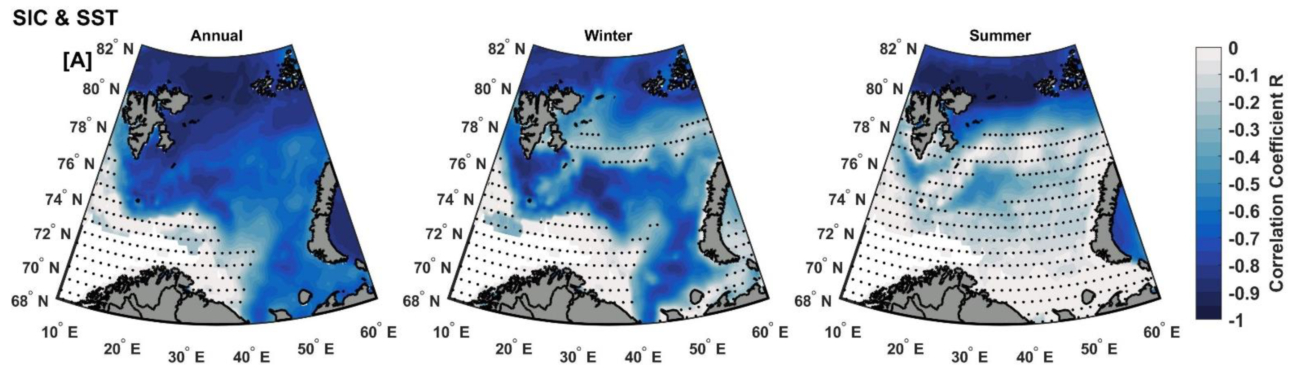
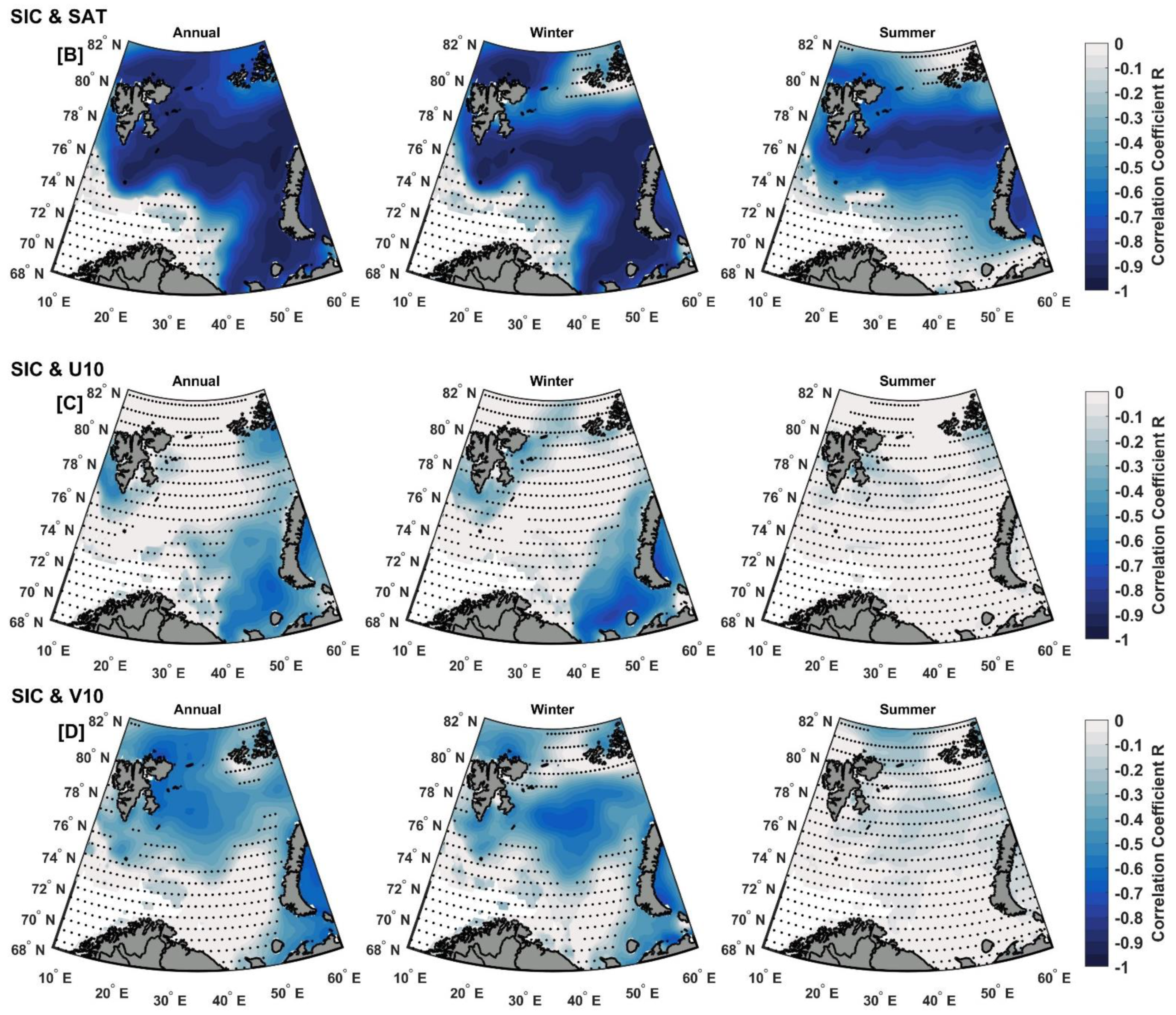
3.5. Correlation Analysis between SST/SIC and Local-Scale Atmospheric Parameters

To investigate the possible role of atmospheric influence and SST on the observed SIC variability in the Barents Sea over the entire record (1982–2020), we investigated the spatiotemporal correlation between SIC with SST and atmospheric parameters (SAT, zonal, and meridional wind components). The temporal correlation coefficients for detrended annual means and non-detrended annual means for all fields are summarized in Table 2 and discussed further below. Figure 15 shows the spatial distribution of detrended annual, winter, and summer correlation coefficients between SIC, SST, and atmospheric parameters. The higher coherence correlation in the spatial distribution of detrended annual correlation maps demonstrates the inverse relationship between SIC with SST and SAT for each grid point of the SIC data in the Barents Sea (Figure 15A,B in the left panel). In winter, these correlations are still significant over most of the Barents Sea (Figure 15A,B in the middle panel), with higher correlation values for SAT than for SST. The higher correlation with SAT indicates that SAT in the Barents Sea is very sensitive to the variability of SIC, especially in the regions where there is a stronger SIC decrease. In summer, the SIC and SST show significant correlation only over the northern part of the Barents Sea (Figure 15A in the right panel), while SIC and SAT are still significant over most of the Barents Sea, with the highest value in the central Barents Sea (Figure 15B in the right panel). The temporal relationship between detrended annual SIC and SST (R = −0.82, Table 2) and SAT (R = −0.93, Table 2) shows that both oceanic and atmospheric warming have a significant impact on sea-ice loss in the Barents Sea.
The temporal correlations between SIC and the zonal wind component are not significant for both the detrended and non-detrended annual mean (Table 2). However, spatial correlation shows a significant correlation between them in the southeastern Barents Sea at annual and winter scales (Figure 15C). This could be due to southwesterly winter winds at the BSO, which increase the inflow of warm AW into the Barents Sea in response to the Ekman transport [75] and lead to the decline of sea ice in this region. On the annual scale, there is a statistically significant correlation between meridional wind and SIC (R = −0.57), SST (R = 0.59), and SAT (R = 0.69). These correlations were reduced but still significant once the trends were not removed (Table 2). On the annual scale, a significant spatial correlation was found between SIC and meridional wind over most of the Barents Sea, with the highest value in the north and east of Svalbard and in the Kara Sea (Figure 15D). The detrended winter SIC significantly correlated with the meridional wind over most of the Barents Sea (Figure 15D in the middle panel), except in the north part of the region between Frans Josef Land and Svalbard, show a non-significant correlation. Strong southerly winter winds (Figure S1H) contributed to increased warming of the area by increasing the advection of warm AW and warm air masses from the south into the northern Barents Sea, reducing SIC. In summer, wind speeds were low, and wind direction was not well defined (Figure S1I), and both zonal and meridional wind components showed a non-significant correlation with SIC (Figure 15). This suggests that summer winds affect sea ice less than winter winds, and thus sea ice in summer depends mainly on the heat flux of the Atlantic inflow into the Barents Sea [46].

4. Conclusions

Here, we analyzed SST, SIC, and meteorological parameters (SAT and zonal and meridional wind components) in the Barents Sea and its sub-basins (ice-covered and ice-free zones) from 1982 to 2020, to describe their evolution, relate them to climate variability (i.e., the teleconnection patterns), identify their possible interrelationships, and examine the impact of atmospheric forcing on SST and sea-ice conditions and trends. We also examined, for the first time to our knowledge, the duration and trend of the sea-ice season in the Barents Sea. The main results are summarized below.
During the cold period P1 (1982–1994), a non-significant trend in oceanic and atmospheric temperatures and sea ice concentration was observed, while during the transition period P2 (1995–2007), the Barents Sea experienced the largest decrease in sea ice associated with a warming of the air-ice-ocean system. Then, in the last period, P3 (2008–2020), these trends were smaller than in period P2. Overall, the SST warming trend from 1982 to 2020 was about 0.35 ± 0.04 °C/decade and 0.40 ± 0.04 °C/decade in the ice-covered and ice-free regions, respectively. However, this warming trend was not spatially homogeneous and varied throughout different historical periods. This climate warming had significant impacts on sea-ice conditions in the Barents Sea, such as a strong decline in the SIC trend (−6.52 ± 0.78%/decade) and a shortening of the sea-ice season by about −26.1 ± 7.5 days/decade, resulting in a 3.4-months longer ice-free season over the last 39 years. The SIC trends in the Barents Sea were generally characterized by significant seasonal and spatial variations. The greatest sea-ice loss occurred in winter with a trend of −8.15 ± 2.40%/decade, which was more than twice the summer trend of −4.00 ± 1.96%/decade. A phenological shift (i.e., seasonal timing transition) was observed in the SST seasonal cycle (Figure 6), with a significant trend toward warmer and longer summer periods (+1.32 ± 0.49 days/year). This is expected to have important ecological impacts.
For both SST and SIC, we found pronounced variability on the 5–6 years (centered at about 5.4 years) and 10.7-year time scales (Figure 14A,B). Both indicated the presence of multidecadal variability. According to the variance analysis, the interannual variability of SST and SIC accounts for about 6.5% and 12% of the total variance of SST and SIC, respectively (Figure S3), with higher interannual variability over the polar front and in regions affected by the inflow of warm Atlantic water.
Empirical orthogonal function analysis (EOF) was performed to investigate interannual to multi-decadal SST and SIC variability in the Barents Sea from 1982 to 2020. The first EOF mode of SST (explains 72% of the total non-seasonal variance) and SIC (explains 68%) show that the Barents Sea has strong coherent interannual spatiotemporal variability of both SST and SIC, with a correlation (R = −0.85) between their first EOF principal component (PC1). The spatial distribution pattern of this mode captures an in-phase fluctuation across the entire Barents Sea, with positive/negative anomalies for SST/SIC across the basin (i.e., in-phase warming implying a decline in SIC across the basin). The center of action for the first mode (i.e., the largest spatial variability) of SST is observed over the polar front regions, while for SIC, it was found over the northeastern Barents Sea and the Storbank and Olga Basin. The second EOF mode of SST (explains 8%) and SIC (explains 12%) indicate a dipole structure with out-of-phase variability between the ice-covered and ice-free regions for SST and between the Svalbard and Novaya Zemlya regions for SIC. On the interannual time scale, significant spatial and temporal correlations were found between SST and SIC and their first EOF mode with two climate indices (AMO and EAP). This indicates that throughout the 39-year study period, SST and SIC variability could be attributed to the AMO, and atmospheric changes are driven by EAP climate modes. The NAO, on the other hand, correlated only with the second EOF mode of SST on the decadal scale (Table 1).
From the correlation analysis (Table 1 and Table 2 and Figure 14 and Figure 15) and the correspondence of the spatial trend pattern of SIC (Figure 10A–C) with atmospheric temperature and wind (Figure 11A–C). In general, we conclude that in addition to the role of warm AW inflow into the Barents Sea, which has been well documented in several previous studies [16,20,25,75,80], local atmospheric circulations and large-scale atmospheric patterns most likely play an important role in the SIC variability and trend in the Barents Sea. This effect is either directly, i.e., north–south meridional winds redistributing sea ice and bringing warm air masses over the Barents Sea, or indirectly with an increase/decrease in the inflow of AW into the Barents Sea. Particularly during winter, the strong southerly winds reduced the sea-ice transport from the Arctic to the Barents Sea and contributed to stronger atmospheric warming of the Barents Sea.

Supplementary Materials

The following are available online at https://www.mdpi.com/article/10.3390/rs14174413/s1, Figure S1: Spatial maps of climatological mean SST (upper panels), SIC (middle panels), and SAT with corresponding mean surface winds (arrows) overlaid (lower panels). (A, D, and G) overall, (B, E, and H) in winter, and (C, F, and I) in summer between 1982 and 2020. Figure S2: Monthly and annual trend of (A) SST and (B) SIC for the period 1982–2020. Error bars showing 95 % confidence intervals. Figure S3: Percentage of the variance explained by the interannual variability of (A) SST and (B) SIC. Figure S4: Lag-lead correlation of the first principal component of SST (red), SIC (blue), and AMO index shows a nearly symmetric shape centered around lag = 33 months, suggesting that the coupled variability is characterized by a linear response of SST/SIC to AMO index. Figure S5A: Normalized annual time series of the first principal component (PC1) of the SST anomalies (red dotted line) along with (A) the AMO index (blue dotted line) along with (B) the EAP (black dotted line) over the period 1982–2020, along with their corresponding six-year running averages (solid lines); Figure S5B: The same as Figure S5A for SIC. Figure S5C: Normalized annual time series of the second principal component (PC2) of the SST anomalies (red dotted line) along with (A) the NAO index (green dotted line) over the period 1982–2020, along with their corresponding six-year running averages (solid lines). Figure S6: Power spectra of the filtered (13-month running mean) and de-trended monthly anomaly of the spatially averaged (A) SST and (B) SIC time series for the period from 1982 to 2020. The time series are smoothed using a 13-month running mean to remove signals with periods shorter than 1 year. The vertical dashed lines show the period of maximum variance centered at 5.4 and 10.7 years for SST and SIC. Figure S7: Simultaneous (a) SST and (b) SAT anomalies (in °C) over the period from 1982 through 2020. The spatially averaged time series showed significantly higher air temperature anomalies than SST during the last two decades, indicating the potential importance of changes in relevant atmospheric and oceanic processes.

Author Contributions

B.M., F.N. and R.S.: conceptualization, methodology, software, validation of results, formal analysis, investigation, resources, data curation, writing, review, editing, and visualization. B.M.: writing—original draft preparation. F.N. and R.S.: supervision, project administration, and funding acquisition. All authors have read and agreed to the published version of the manuscript.

Funding

This work was fully funded by the Research Council of Norway through the Nansen Legacy Project (RCN # 276730).

Data Availability Statement

The original contributions presented in the study are included in the article and Supplementary Materials, further inquiries can be directed to the corresponding author.

Acknowledgments

We would like to thank the organizations that provided the data used in this work, including the Copernicus Marine Environment Monitoring Service (CMEMS) for SST and SIC data, the National Oceanic and Atmospheric Administration (NOAA) for climate indices, and the European Centre for Medium-Range Weather Forecasts (ECMWF) for atmospheric parameters. The authors would like to thank Léon Chafik (Stockholm University, Sweden) for his valuable comments on the earliest version of this manuscript and explanation AMO index results. We would also like to express our gratitude to the anonymous reviewers for their contributions to the development of this manuscript.

Conflicts of Interest

The authors declare no conflict of interest. The funders had no role in the design of the study; in the collection, analyses, or interpretation of data; in the writing of the manuscript, or in the decision to publish the results.

References

  1. Serreze, M.C.; Barry, R.G. Processes and impacts of Arctic amplification: A research synthesis. Glob. Planet. Chang. 2011, 77, 85–96. [Google Scholar] [CrossRef]
  2. Schweiger, A.J.; Wood, K.R.; Zhang, J. Arctic Sea Ice Volume Variability over 1901–2010: A Model-Based Reconstruction. J. Clim. 2019, 32, 4731–4752. [Google Scholar] [CrossRef]
  3. Serreze, M.C.; Barrett, A.P.; Stroeve, J.C.; Kindig, D.N.; Holland, M.M. The emergence of surface-based Arctic amplification. Cryosphere 2009, 3, 11–19. [Google Scholar] [CrossRef]
  4. Kohnemann, S.H.E.; Heinemann, G.; Bromwich, D.H.; Gutjahr, O. Extreme Warming in the Kara Sea and Barents Sea during the Winter Period 2000–16. J. Clim. 2017, 30, 8913–8927. [Google Scholar] [CrossRef]
  5. Stroeve, J.; Notz, D. Changing state of Arctic sea ice across all seasons. Environ. Res. Lett. 2018, 13, 103001. [Google Scholar] [CrossRef]
  6. Serreze, M.C.; Meier, W.N. The Arctic’s sea ice cover: Trends, variability, predictability, and comparisons to the Antarctic. Ann. N. Y. Acad. Sci. 2019, 1436, 36–53. [Google Scholar] [CrossRef] [PubMed]
  7. Lind, S.; Ingvaldsen, R.B.; Furevik, T. Arctic warming hotspot in the northern Barents Sea linked to declining sea-ice import. Nat. Clim. Chang. 2018, 8, 634–639. [Google Scholar] [CrossRef]
  8. Screen, J.A.; Simmonds, I. The central role of diminishing sea ice in recent Arctic temperature amplification. Nature 2010, 464, 1334–1337. [Google Scholar] [CrossRef]
  9. Cohen, J.; Screen, J.A.; Furtado, J.C.; Barlow, M.; Whittleston, D.; Coumou, D.; Francis, J.; Dethloff, K.; Entekhabi, D.; Overland, J.; et al. Recent Arctic amplification and extreme mid-latitude weather. Nat. Geosci. 2014, 7, 627–637. [Google Scholar] [CrossRef]
  10. Parkinson, C.L. Spatially mapped reductions in the length of the Arctic sea ice season. Geophys. Res. Lett. 2014, 41, 4316–4322. [Google Scholar] [CrossRef] [Green Version]
  11. Stroeve, J.C.; Markus, T.; Boisvert, L.; Miller, J.; Barrett, A. Changes in Arctic melt season and implications for sea ice loss. Geophys. Res. Lett. 2014, 41, 1216–1225. [Google Scholar] [CrossRef]
  12. Lebrun, M.; Vancoppenolle, M.; Madec, G.; Massonnet, F. Arctic sea-ice-free season projected to extend into autumn. Cryosphere 2019, 13, 79–96. [Google Scholar] [CrossRef]
  13. Schlichtholz, P. Subsurface ocean flywheel of coupled climate variability in the Barents Sea hotspot of global warming. Sci. Rep. 2019, 9, 13692. [Google Scholar] [CrossRef]
  14. Årthun, M.; Onarheim, I.H.; Dörr, J.; Eldevik, T. The Seasonal and Regional Transition to an Ice-Free Arctic. Geophys. Res. Lett. 2021, 48, e2020GL090825. [Google Scholar] [CrossRef]
  15. Onarheim, I.H.; Eldevik, T.; Smedsrud, L.H.; Stroeve, J.C. Seasonal and regional manifestation of Arctic sea ice loss. J. Clim. 2018, 31, 4917–4932. [Google Scholar] [CrossRef]
  16. Årthun, M.; Eldevik, T.; Smedsrud, L.H.; Skagseth, Ø.; Ingvaldsen, R.B. Quantifying the Influence of Atlantic Heat on Barents Sea Ice Variability and Retreat. J. Clim. 2012, 25, 4736–4743. [Google Scholar] [CrossRef]
  17. Oziel, L.; Neukermans, G.; Ardyna, M.; Lancelot, C.; Tison, J.-L.; Wassmann, P.; Sirven, J.; Ruiz-Pino, D.; Gascard, J.-C. Role for Atlantic inflows and sea ice loss on shifting phytoplankton blooms in the Barents Sea. J. Geophys. Res. Ocean. 2017, 122, 5121–5139. [Google Scholar] [CrossRef]
  18. Herbaut, C.; Houssais, M.N.; Close, S.; Blaizot, A.C. Two wind-driven modes of winter sea ice variability in the Barents Sea. Deep. Res. Part I Oceanogr. Res. Pap. 2015, 106, 97–115. [Google Scholar] [CrossRef]
  19. Mohamed, B.; Nilsen, F.; Skogseth, R. Marine Heatwaves Characteristics in the Barents Sea Based on High Resolution Satellite Data (1982–2020). Front. Mar. Sci. 2022, 9, 1–17. [Google Scholar] [CrossRef]
  20. Skagseth, Ø.; Eldevik, T.; Årthun, M.; Asbjørnsen, H.; Lien, V.S.; Smedsrud, L.H. Reduced efficiency of the Barents Sea cooling machine. Nat. Clim. Chang. 2020, 10, 661–666. [Google Scholar] [CrossRef]
  21. Pecuchet, L.; Jørgensen, L.L.; Dolgov, A.V.; Eriksen, E.; Husson, B.; Skern-Mauritzen, M.; Primicerio, R. Spatio-temporal turnover and drivers of bentho-demersal community and food web structure in a high-latitude marine ecosystem. Divers. Distrib. 2022, 00, 1–18. [Google Scholar] [CrossRef]
  22. Husson, B.; Lind, S.; Fossheim, M.; Kato-Solvang, H.; Skern-Mauritzen, M.; Pécuchet, L.; Ingvaldsen, R.B.; Dolgov, A.V.; Primicerio, R. Successive extreme climatic events lead to immediate, large-scale, and diverse responses from fish in the Arctic. Glob. Chang. Biol. 2022, 28, 3728–3744. [Google Scholar] [CrossRef]
  23. Schlichtholz, P. Influence of oceanic heat variability on sea ice anomalies in the Nordic Seas. Geophys. Res. Lett. 2011, 38, 5705. [Google Scholar] [CrossRef]
  24. Koenigk, T.; Mikolajewicz, U.; Jungclaus, J.H.; Kroll, A. Sea ice in the Barents Sea: Seasonal to interannual variability and climate feedbacks in a global coupled model. Clim. Dyn. 2009, 32, 1119–1138. [Google Scholar] [CrossRef]
  25. Efstathiou, E.; Eldevik, T.; Årthun, M.; Lind, S. Spatial Patterns, Mechanisms, and Predictability of Barents Sea Ice Change. J. Clim. 2022, 35, 2961–2973. [Google Scholar] [CrossRef]
  26. Sorteberg, A.; Kvingedal, B. Atmospheric Forcing on the Barents Sea Winter Ice Extent. J. Clim. 2006, 19, 4772–4784. [Google Scholar] [CrossRef]
  27. Lind, S.; Ingvaldsen, R.B.; Furevik, T. Arctic layer salinity controls heat loss from deep Atlantic layer in seasonally ice-covered areas of the Barents Sea. Geophys. Res. Lett. 2016, 43, 5233–5242. [Google Scholar] [CrossRef]
  28. Onarheim, I.H.; Eldevik, T.; Årthun, M.; Ingvaldsen, R.B.; Smedsrud, L.H. Skillful prediction of Barents Sea ice cover. Geophys. Res. Lett. 2015, 42, 5364–5371. [Google Scholar] [CrossRef]
  29. Lien, V.S.; Schlichtholz, P.; Skagseth, Ø.; Vikebø, F.B. Wind-Driven Atlantic Water Flow as a Direct Mode for Reduced Barents Sea Ice Cover. J. Clim. 2017, 30, 803–812. [Google Scholar] [CrossRef]
  30. Chernokulsky, A.V.; Esau, I.; Bulygina, O.N.; Davy, R.; Mokhov, I.I.; Outten, S.; Semenov, V.A. Climatology and Interannual Variability of Cloudiness in the Atlantic Arctic from Surface Observations since the Late Nineteenth Century. J. Clim. 2017, 30, 2103–2120. [Google Scholar] [CrossRef]
  31. Wei, J.; Zhang, X.; Wang, Z. Impacts of extratropical storm tracks on Arctic sea ice export through Fram Strait. Clim. Dyn. 2019, 52, 2235–2246. [Google Scholar] [CrossRef]
  32. Boisvert, L.N.; Petty, A.A.; Stroeve, J.C. The Impact of the Extreme Winter 2015/16 Arctic Cyclone on the Barents–Kara Seas. Mon. Weather Rev. 2016, 144, 4279–4287. [Google Scholar] [CrossRef]
  33. Schlichtholz, P. Local Wintertime Tropospheric Response to Oceanic Heat Anomalies in the Nordic Seas Area. J. Clim. 2014, 27, 8686–8706. [Google Scholar] [CrossRef]
  34. Woods, C.; Caballero, R. The Role of Moist Intrusions in Winter Arctic Warming and Sea Ice Decline. J. Clim. 2016, 29, 4473–4485. [Google Scholar] [CrossRef]
  35. Zhang, X.; Sorteberg, A.; Zhang, J.; Gerdes, R.; Comiso, J.C. Recent radical shifts of atmospheric circulations and rapid changes in Arctic climate system. Geophys. Res. Lett. 2008, 35, 22701. [Google Scholar] [CrossRef]
  36. Yashayaev, I.; Seidov, D. The role of the Atlantic Water in multidecadal ocean variability in the Nordic and Barents Seas. Prog. Oceanogr. 2015, 132, 68–127. [Google Scholar] [CrossRef]
  37. Skagseth, Ø.; Furevik, T.; Ingvaldsen, R.; Loeng, H.; Mork, K.A.; Orvik, K.A.; Ozhigin, V. Volume and Heat Transports to the Arctic Ocean Via the Norwegian and Barents Seas. In Arctic–Subarctic Ocean Fluxes; Springer: Dordrecht, The Netherlands, 2008; pp. 45–64. [Google Scholar] [CrossRef]
  38. Trenberth, K.E.; Shea, D.J. Atlantic hurricanes and natural variability in 2005. Geophys. Res. Lett. 2006, 33, 12704. [Google Scholar] [CrossRef]
  39. Levitus, S.; Matishov, G.; Seidov, D.; Smolyar, I. Barents Sea multidecadal variability. Geophys. Res. Lett. 2009, 36, 19604. [Google Scholar] [CrossRef]
  40. Oziel, L.; Sirven, J.; Gascard, J.C. The Barents Sea frontal zones and water masses variability (1980–2011). Ocean Sci. 2016, 12, 169–184. [Google Scholar] [CrossRef] [Green Version]
  41. Hurrell, J.W.; Kushnir, Y.; Ottersen, G.; Visbeck, M. An Overview of the North Atlantic Oscillation. Geophys. Monogr. Ser. 2003, 134, 1–35. [Google Scholar] [CrossRef]
  42. Chafik, L.; Nilsson, J.; Skagseth, Ø.; Lundberg, P. On the flow of Atlantic water and temperature anomalies in the Nordic Seas toward the Arctic Ocean. J. Geophys. Res. Ocean. 2015, 120, 7897–7918. [Google Scholar] [CrossRef]
  43. Muilwijk, M.; Smedsrud, L.H.; Ilicak, M.; Drange, H. Atlantic Water Heat Transport Variability in the 20th Century Arctic Ocean From a Global Ocean Model and Observations. J. Geophys. Res. Ocean. 2018, 123, 8159–8179. [Google Scholar] [CrossRef]
  44. Barnston, A.G.; Livezey, R.E. Classification, Seasonality and Persistence of Low-Frequency Atmospheric Circulation Patterns. Mon. Weather Rev. 1987, 115, 1083–1126. [Google Scholar] [CrossRef]
  45. King, J.; Spreen, G.; Gerland, S.; Haas, C.; Hendricks, S.; Kaleschke, L.; Wang, C. Sea-ice thickness from field measurements in the northwestern Barents Sea. J. Geophys. Res. Ocean. 2017, 122, 1497–1512. [Google Scholar] [CrossRef]
  46. Pavlova, O.; Pavlov, V.; Gerland, S. The impact of winds and sea surface temperatures on the Barents Sea ice extent, a statistical approach. J. Mar. Syst. 2014, 130, 248–255. [Google Scholar] [CrossRef]
  47. Kumar, A.; Yadav, J.; Mohan, R. Spatio-temporal change and variability of Barents-Kara sea ice, in the Arctic: Ocean and atmospheric implications. Sci. Total Environ. 2021, 753, 142046. [Google Scholar] [CrossRef]
  48. Duan, C.; Dong, S.; Xie, Z.; Wang, Z. Temporal variability and trends of sea ice in the Kara Sea and their relationship with atmospheric factors. Polar Sci. 2019, 20, 136–147. [Google Scholar] [CrossRef]
  49. Jiang, Z.; Feldstein, S.B.; Lee, S. Two Atmospheric Responses to Winter Sea Ice Decline Over the Barents-Kara Seas. Geophys. Res. Lett. 2021, 48, e2020GL090288. [Google Scholar] [CrossRef]
  50. Sakshaug, E.; Johnsen, G.; Kristiansen, S.; Von, C.; Rey, F.; Slagstad, D.; Thingstad, F. Ecosystem Barents Sea; Tapir Academic Press: Trondheim, Norway, 2009; ISBN 9788251924610. [Google Scholar]
  51. Good, S.; Fiedler, E.; Mao, C.; Martin, M.J.; Maycock, A.; Reid, R.; Roberts-Jones, J.; Searle, T.; Waters, J.; While, J.; et al. The current configuration of the OSTIA system for operational production of foundation sea surface temperature and ice concentration analyses. Remote Sens. 2020, 12, 720. [Google Scholar] [CrossRef] [Green Version]
  52. Hersbach, H.; Bell, B.; Berrisford, P.; Hirahara, S.; Horányi, A.; Muñoz-Sabater, J.; Nicolas, J.; Peubey, C.; Radu, R.; Schepers, D.; et al. The ERA5 global reanalysis. Q. J. R. Meteorol. Soc. 2020, 146, 1999–2049. [Google Scholar] [CrossRef]
  53. Hannachi, A.; Jolliffe, I.T.; Stephenson, D.B. Empirical orthogonal functions and related techniques in atmospheric science: A review. Int. J. Climatol. 2007, 27, 1119–1152. [Google Scholar] [CrossRef]
  54. Thomson, R.E.; Emery, W.J. Data Analysis Methods in Physical Oceanography, 3rd ed.; Elsevier Inc.: Amsterdam, The Netherlands, 2014; ISBN 9780123877833. [Google Scholar]
  55. Meyssignac, B.; Piecuch, C.G.; Merchant, C.J.; Racault, M.F.; Palanisamy, H.; MacIntosh, C.; Sathyendranath, S.; Brewin, R. Causes of the Regional Variability in Observed Sea Level, Sea Surface Temperature and Ocean Colour Over the Period 1993–2011. Surv. Geophys. 2017, 38, 187–215. [Google Scholar] [CrossRef]
  56. Barton, B.I.; Lenn, Y.D.; Lique, C. Observed atlantification of the Barents Sea causes the Polar Front to limit the expansion of winter sea ice. J. Phys. Oceanogr. 2018, 48, 1849–1866. [Google Scholar] [CrossRef]
  57. Schlegel, R.W.; Smit, A.J. Climate change in coastal waters: Time series properties affecting trend estimation. J. Clim. 2016, 29, 9113–9124. [Google Scholar] [CrossRef]
  58. Levine, R.A.; Wilks, D.S. Statistical Methods in the Atmospheric Sciences; Academic Press: Cambridge, MA, USA, 2000; Volume 95, ISBN 0123850223. [Google Scholar]
  59. Emery, W.J.; Thomson, R.E. Data Analysis Methods in Physical Oceanography; Newnes: London, UK, 1997; ISBN 0080314341. [Google Scholar]
  60. Hamed, K.H.; Ramachandra Rao, A. A modified Mann-Kendall trend test for autocorrelated data. J. Hydrol. 1998, 204, 182–196. [Google Scholar] [CrossRef]
  61. Wang, F.; Shao, W.; Yu, H.; Kan, G.; He, X.; Zhang, D.; Ren, M.; Wang, G. Re-evaluation of the Power of the Mann-Kendall Test for Detecting Monotonic Trends in Hydrometeorological Time Series. Front. Earth Sci. 2020, 8, 14. [Google Scholar] [CrossRef]
  62. Greene, C.A.; Thirumalai, K.; Kearney, K.A.; Delgado, J.M.; Schwanghart, W.; Wolfenbarger, N.S.; Thyng, K.M.; Gwyther, D.E.; Gardner, A.S.; Blankenship, D.D. The Climate Data Toolbox for MATLAB. Geochem. Geophys. Geosys. 2019, 20, 3774–3781. [Google Scholar] [CrossRef]
  63. Wang, Y.; Bi, H.; Huang, H.; Liu, Y.; Liu, Y.; Liang, X.; Fu, M.; Zhang, Z. Satellite-observed trends in the Arctic sea ice concentration for the period 1979–2016. J. Oceanol. Limnol. 2018, 37, 18–37. [Google Scholar] [CrossRef]
  64. Krauzig, N.; Falco, P.; Zambianchi, E. Contrasting surface warming of a marginal basin due to large-scale climatic patterns and local forcing. Sci. Rep. 2020, 10, 17648. [Google Scholar] [CrossRef]
  65. Pärn, O.; Friedland, R.; Rjazin, J.; Stips, A. Regime shift in sea-ice characteristics and impact on the spring bloom in the Baltic Sea. Oceanologia 2021, 64, 312–326. [Google Scholar] [CrossRef]
  66. Stammerjohn, S.E.; Martinson, D.G.; Smith, R.C.; Yuan, X.; Rind, D. Trends in Antarctic annual sea ice retreat and advance and their relation to El Niño–Southern Oscillation and Southern Annular Mode variability. J. Geophys. Res. Ocean. 2008, 113, 3–90. [Google Scholar] [CrossRef]
  67. von Storch, H.; Zwiers, F.W. Statistical Analysis in Climate Research; Cambridge University Press: Cambridge, UK, 1999. [Google Scholar] [CrossRef]
  68. Asbjørnsen, H.; Årthun, M.; Skagseth, Ø.; Eldevik, T. Mechanisms Underlying Recent Arctic Atlantification. Geophys. Res. Lett. 2020, 47, e2020GL088036. [Google Scholar] [CrossRef]
  69. Koul, V.; Brune, S.; Baehr, J.; Schrum, C. Impact of Decadal Trends in the Surface Climate of the North Atlantic Subpolar Gyre on the Marine Environment of the Barents Sea. Front. Mar. Sci. 2022, 8, 2065. [Google Scholar] [CrossRef]
  70. Onarheim, I.H.; Smedsrud, L.H.; Ingvaldsen, R.B.; Nilsen, F. Loss of sea ice during winter north of Svalbard. Tellus Ser. A Dyn. Meteorol. Oceanogr. 2014, 66, 1–9. [Google Scholar] [CrossRef]
  71. Smedsrud, L.H.; Esau, I.; Ingvaldsen, R.B.; Eldevik, T.; Haugan, P.M.; Li, C.; Lien, V.S.; Olsen, A.; Omar, A.M.; Risebrobakken, B.; et al. The role of the Barents Sea in the Arctic climate system. Rev. Geophys. 2013, 51, 415–449. [Google Scholar] [CrossRef]
  72. Ivanov, V.; Alexeev, V.; Koldunov, N.V.; Repina, I.; Sandø, A.B.; Smedsrud, L.H.; Smirnov, A. Arctic Ocean Heat Impact on Regional Ice Decay: A Suggested Positive Feedback. J. Phys. Oceanogr. 2016, 46, 1437–1456. [Google Scholar] [CrossRef]
  73. Aagaarda, K.; Foldvik, A.; Hillman, S.R. The West Spitsbergen Current: Disposition and water mass transformation. J. Geophys. Res. Ocean. 1987, 92, 3778–3784. [Google Scholar] [CrossRef]
  74. Nilsen, F.; Skogseth, R.; Vaardal-Lunde, J.; Inall, M. A Simple Shelf Circulation Model: Intrusion of Atlantic Water on the West Spitsbergen Shelf. J. Phys. Oceanogr. 2016, 46, 1209–1230. [Google Scholar] [CrossRef]
  75. Lien, V.S.; Vikebø, F.B.; Skagseth, Ø. One mechanism contributing to co-variability of the Atlantic inflow branches to the Arctic. Nat. Commun. 2013, 4, 1488. [Google Scholar] [CrossRef]
  76. Torres, R.R.; Tsimplis, M.N. Sea-level trends and interannual variability in the Caribbean Sea. J. Geophys. Res. Ocean. 2013, 118, 2934–2947. [Google Scholar] [CrossRef]
  77. Mohamed, B.; Skliris, N. Steric and atmospheric contributions to interannual sea level variability in the eastern mediterranean sea over 1993–2019. Oceanologia 2022, 64, 50–62. [Google Scholar] [CrossRef]
  78. Welch, P.D. The Use of Fast Fourier Transform for the Estimation of Power Spectra: A Method Based on Time Averaging Over Short, Modified Periodograms. IEEE Trans. Audio Electroacoust. 1967, 15, 70–73. [Google Scholar] [CrossRef]
  79. Perlwitz, J.; Knutson, T.; Kossin, J.P.; LeGrande, A.N. Chapter 5: Large-Scale Circulation and Climate Variability. In Climate Science Special Report: Fourth National Climate Assessment; U.S. Global Change Research Program: Washington, DC, USA, 2017; Volume I, pp. 161–184. [Google Scholar] [CrossRef]
  80. Årthun, M.; Eldevik, T. On anomalous ocean heat transport toward the Arctic and associated climate predictability. J. Clim. 2016, 29, 689–704. [Google Scholar] [CrossRef]
Figure 1. Map of the Barents Sea with bathymetry (GEBCO, https://www.gebco.net (accessed on 30 May 2022)). The Barents Sea was divided into two regions: the ice-covered zone (ICZ, in the north), and the ice-free zone (IFZ, in the south), based on the climatological mean of the April sea-ice concentration edge (15% SIC, solid white line) for the entire period (1982–2020). Isobaths of 100, 220, 300, and 500 m are shown in black. Abbreviations stand for the Barents Sea Opening (BSO), Bear Island Trough (BIT), Hopen Trough (HT), Bear Island (BI), Storfjorden Trough (SFT), Kong Karls Land (KKL), Olga Basin (OB), Franz Joseph Land (FJL), and the St. Anna Trough (St.AT). The Kola Section (KS) is marked with a straight green line.
Remotesensing 14 04413 g001
Figure 2. The climatological mean of SST (upper panels) and SIC (lower panels) for the periods; (A,D) P1 (1982–1994), (B,E) P2 (1995–2007), and (C,F) P3 (2008–2020). The contour lines are indicated by the respective labels to the right.
Remotesensing 14 04413 g002
Figure 3. Average daily seasonal curves of (A) SST and (B) SIC over the whole Barents Sea for the periods P1 (1982–1994, blue line), P2 (1995–2007, green line), and P3 (2008–2020, red line). The red and blue bars in (A,B) indicate the daily increase/decrease of SST and SIC between P3 and P1. The seasonal curve changes demonstrate that the summer season began earlier and lasted longer, with SST increases exceeding 1 °C through October and November between P1 and P3, while the lowest SST increase (~0.55 °C) was found through March and April. The horizontal dotted black line in (A) represents the 3.6 °C threshold of SST.
Remotesensing 14 04413 g003aRemotesensing 14 04413 g003b
Figure 4. Spatially averaged daily SST (A) and SIC (B) with time indicating changes in the seasonal cycles during 1982–2020.
Remotesensing 14 04413 g004
Figure 5. Changes in SST phenology over the entire Barents Sea for the 39 years (1982–2020), demonstrating the trend of (A) the duration of the warm season, and the start (B) and the end (C) date of the warm season.
Remotesensing 14 04413 g005
Figure 6. Average duration of sea-ice season (in Days) for (A) the whole period (1982–2020), (B) the beginning (1982), and (C) the end (2020) year of the period.
Remotesensing 14 04413 g006
Figure 7. Average annual duration of the sea-ice season in the Barents Sea ((A), blue line) and its temporal ((A), black line) and spatial ((B), shading) trends (in days/year) from 1982 to 2020.
Remotesensing 14 04413 g007aRemotesensing 14 04413 g007b
Figure 8. Spatial distribution of averaged de-seasoned trends of SST (top panel), SIC (middle panel), and SAT with corresponding trends of surface winds (arrows) overlaid (bottom panel). (A,D,G) overall, (B,E,H) in winter, and (C,F,I) in summer between 1982 and 2020. The white region in the middle panel indicates that SIC was below the climatological mean for the April sea-ice edge (15%) throughout the entire period. Non-significant values are indicated by black dots.
Remotesensing 14 04413 g008
Figure 9. Spatial distribution of the de-seasoned trends of SSTA for the periods; (A) P1 (1982–1994), (B) P2 (1995–2007), and (C) P3 (2008–2020), respectively. Regions where the trends are not statistically significant at the 95% confidence interval (after Mann–Kendall’s test) are stippled. De-seasoned monthly mean time series of spatially averaged SSTA over (D) the ice-covered zone (ICZ) and (E) the ice-free zone (IFZ) from 1982 through 2020. Trends for each period (colored dashed lines) and for the entire period (black solid line) are also shown. To enhance the visualization and to emphasize interannual variability, the data was low-passed using a 13-month moving average (red line).
Remotesensing 14 04413 g009
Figure 10. Spatial distribution of the de-seasoned trends of SICA for the periods; (A) P1 (1982–1994), (B) P2 (1995–2007), and (C) P3 (2008–2020), respectively. Regions where the trends are not statistically significant at the 95% confidence interval (after Mann–Kendall’s test) are stippled. The red lines represent the mean April sea-ice edge (15% SIC) for each period. (D) De-seasoned monthly mean time series of spatially averaged SICA over the ice-covered zone from 1982 through 2020. Trends for each period (colored dashed lines) and for the entire period (black solid line) are also shown. To enhance the visualization and to emphasize interannual variability, the data was low passed using a 13-month moving average (red line).
Remotesensing 14 04413 g010
Figure 11. Spatial distribution of the de-seasoned trends of SATA for the periods; (A) P1 (1982–1994), (B) P2 (1995–2007), and (C) P3 (2008–2020), respectively. Regions where the SAT trends are not statistically significant at the 95% confidence interval (after Mann–Kendall’s test) are stippled. The vectors in the upper panels represent the corresponding trends (unit: (m/s)/13 years) of the surface winds. The reference for wind vectors trend is plotted in (C). (D) De-seasoned monthly mean time series of spatially averaged SATA over the whole Barents Sea from 1982 to 2020. Trends for each period (colored dashed lines) and for the entire period (black solid line) are also shown. To enhance the visualization and to emphasize interannual variability, the data was low-passed using a 13-month moving average (red line).
Remotesensing 14 04413 g011
Figure 12. Spatial pattern of the first (top panel) and second (lower panel) EOF modes of the de-seasoned and filtered (13-month running mean) anomalies of SST (A,B) and SIC (C,D) from 1982 to 2020. The variance explained by each EOF is also given above each panel.
Remotesensing 14 04413 g012
Figure 13. Normalized interannual (13-month running mean) time series of (A) the first principal component (PC1) for SST (red line) and SIC (blue line) anomalies in normalized variance units along with the AMO index (black line) and the EAP (green line) over the period 1982–2020. (B) The second principal component (PC2) for both SST (red line) and SIC (blue line), which are not statistically significantly correlated with any of the climate indices. Note that for SIC, the positive value of PC1SIC and PC2SIC corresponds to the decrease of sea ice (negative SIC anomalies), as we draw the inverted SIC PCs for better visualization.
Remotesensing 14 04413 g013
Figure 14. Spatial distribution of correlation coefficients between the interannual variability of SST (upper panels), SIC (lower panels) with the (A,D) AMO, (B,E) NAO, and (C,F) EAP over the period from 1982 to 2020. All data were filtered with a 13-month low-pass filter after the removal of seasonal climatology and then normalized.
Remotesensing 14 04413 g014
Figure 15. Spatial distribution of correlation coefficients between SIC and (A) sea surface temperature (SST), (B) surface air temperature (SAT), (C) zonal, and (D) meridional wind components over the period from 1982 to 2020. Each line consists of three maps: the left shows (annual), the middle (winter), and the right (summer). Time series at each grid point were detrended before determining correlations.
Remotesensing 14 04413 g015aRemotesensing 14 04413 g015b
Table 1. Correlation coefficients (R) between annual/decadal (6-year running means) normalized SST, SIC, and their leading modes (PC1 and PC2), with the climatic mode indices (AMO, NAO, and EAP). Significant correlations (p-values < 0.05) are highlighted in bold. The maximum correlation and time lag are shown in brackets to the right of R; negative lag refers to the lagged response of SST or SIC (@year) to the AMO index. SSTICZ and SSTIFZ refer to SST over the ice-covered and ice-free zones, respectively.
CorrelationAMO/AMO (6)NAO/NAO (6)EAP/EAP (6)
SST/SST (6)0.52 (0.59@−3)/0.750.04/−0.150.54/0.90
SSTICZ/SSTICZ (6)0.45 (0.51@−3)/0.670.05/−0.100.45/0.86
SSTIFZ/SSTIFZ (6)0.55 (0.64@−3)/0.790.03/−0.160.60/0.92
SIC/SIC (6)−0.43 (−0.54@−3)/−0.740.04/0.23−0.35/−0.83
PC1SST/PC1SST (6)0.53 (0.60@−3)/0.750.04/−0.160.56/0.91
PC2SST/PC2SST (6)−0.27/−0.300.09/0.45−0.19/−0.24
PC1SIC/PC1SIC (6)−0.47 (−0.57@−3)/−0.760.06/0.26−0.44/−0.87
PC2SIC/PC2SIC (6)−0.12/−0.07−0.02/0.06−0.30/−0.31
Table 2. Cross-correlation matrix between annual mean SST, SIC, and atmospheric parameters, including surface air temperature (SAT), zonal, and meridional wind components (U10, V10). The lower left triangle represents the correlations between the detrended time series, while the upper right triangle shows the correlations, including the trends. Significant correlations (p-values < 0.05) are highlighted in bold.
CorrelationSICSSTSATU10V10
SIC1−0.93−0.97−0.23−0.35Non-Detrended
SST−0.8210.940.200.34
SAT−0.930.8510.280.42
U10−0.210.160.281-
V10−0.570.590.69-1
Detrended
Publisher’s Note: MDPI stays neutral with regard to jurisdictional claims in published maps and institutional affiliations.

