Article

Quantitative Assessment of Impact of Climate Change and Human Activities on Streamflow Changes Using an Improved Three-Parameter Monthly Water Balance Model

1
College of Hydraulic and Environmental Engineering, Zhejiang University of Water Resources and Electric Power, Hangzhou 310018, China
2
International Science and Technology Cooperation Base for Utilization and Sustainable Development of Water Resources, Zhejiang University of Water Resources and Electric Power, Hangzhou 310018, China
3
Institute of Hydrology and Water Resources, College of Civil Engineering and Architecture, Zhejiang University, Hangzhou 310058, China
4
Department of Civil, Environmental and Geomatics Engineering, Florida Atlantic University, Boca Raton, FL 33431, USA
*
Author to whom correspondence should be addressed.
Remote Sens. 2022, 14(17), 4411; https://doi.org/10.3390/rs14174411
Submission received: 14 July 2022 / Revised: 13 August 2022 / Accepted: 1 September 2022 / Published: 5 September 2022

Abstract

:
Understanding the impact of climate change and human activities on the hydrological cycle of any watershed can provide a scientific basis for regional water resource planning, flood management, and disaster mitigation. An improved three-parameter hydrological model (CM) based on monthly water balance using an exponential equation to depict the distribution of groundwater storage capacity was developed and evaluated. The model uses Asian Precipitation Highly Resolved Observational Data Integration Towards Evaluation (APHRODITE) rainfall data as input, with the Zhejiang Province as the case application, and the effects of climate change and human activities on streamflow changes were assessed by separating environmental variables in this study. The results indicate that APHRODITE data has excellent monthly accuracy, with a mean correlation coefficient (CC) of more than 0.96 and an average absolute percentage bias (Pbais) of less than 5%. The three models are relatively close in their ability to simulate high flows, but the CM simulated low flow is better than the other two models. Positive and negative Pbais phenomena occur in the CM model in each catchment, and absolute levels are regulated by 5%. Furthermore, the CM model’s average Nash efficiency coefficient (NSE) is greater than 0.9, indicating that it can correctly fulfill the water balance. The results are more consistent throughout multiple catchments in each watershed using Budyko-based and hydrological model technique to evaluate the influence of climate change and human activities on streamflow. Climate change dominated streamflow variations in 18 of the 21 catchments in Zhejiang Province, whereas human activities dominated the rest. The findings of the study will be used to influence the management, development, and usage of water resources in the watershed.

1. Introduction

In recent decades, global climate change and human activities have significantly impacted the quantity, quality, and spatial distribution of water resources. Climate change is expected to disrupt the hydrological cycle, resulting in a regional and temporal redistribution of water resources, with significant implications for rainfall, evaporation, runoff, and soil water content [1,2,3,4,5,6]. Water supply, irrigation, navigation, urban drainage, hydropower generation, flood scheduling, soil and water conservation, and water pollution control will all be impacted by changes in the water cycle [7,8,9,10]. The hydrological cycle mechanisms are influenced by both climate change and human activity. Climate change influences watershed runoff in terms of input conditions, such as regional fluctuations in precipitation and temperature changes, while human activities can modify and affect the subsurface conditions directly or indirectly [3]. Long-term water cycle and water resource distribution have become important issues in water resource planning [11], and the monthly scale water balance model is frequently employed in long-term water resource distribution forecasting [12,13,14,15]. The reconstruction of catchment hydrological structures, forecasting of river runoff variations, the consequences of climate change in the catchment, and the evaluation of seasonal and regional water supply and irrigation demand are all examples of current research on monthly water balance models [16,17,18,19].
The hydrological model is a tool for characterizing and simulating the complex spatial and temporal variability in the conversion of rainfall to runoff from a watershed [20,21]. Hydrological models can be categorized into physical and conceptual models [22]. The physical model enables the study of the changing patterns of hydrological processes using physical scenarios, while the conceptual model is a hydrological model based on physical concepts in hydrological phenomena, as well as empirical formulas [11,23]. According to the degree of description of spatial characteristics, models can be classified as lumped, semi-distributed, and distributed hydrological models. Lumped hydrologic models describe the production of runoff using rainfall by taking the entire watershed into account, and the majority of these models lack the capability to mechanically account for the impact of unevenly distributed rainfall and subsurface conditions on the creation of rainfall runoff [24]. The distributed hydrological model divides the basin into several units based on the different information of climate and subsurface characteristics at each part of the basin, and it has the ability to mechanistically take into account the impact of the uneven spatial distribution of rainfall and subsurface conditions on runoff generation [25,26].
Hydrological models generally use mathematical and physical equations to simplify hydrological processes and model parameters representing watershed characteristics [27]. The number of parameters of hydrological models often decreases as the time scale increases. The daily Xinanjiang model, for example, includes 12 parameters, but the monthly ABCD model has only four [28]. The monthly water balance model provides a fundamental generalization of the catchment’s hydrological processes, with relatively minimal model input requirements and quick estimates with a few model parameters [29,30,31]. Thornthwaite [32] developed the first monthly water balance model in the 1940s, which was later improved by Thornthwaite and Mather [33]. Many water-balance models based on various assumptions and model architectures were sequentially suggested by researchers to accommodate hydrological simulations with varied aims, such as drought analysis, water quantity estimation, and ecological studies [34,35,36]. For example, considering Thomas’s [37] well-known ABCD monthly water balance model, Makhlouf and Michel [38] proposed the GR2M two-parameter monthly water balance model for evaluating and managing water resources, and Xiong and Guo [39] studied a two-parameter monthly water balance model and utilized it to simulate streamflow in Southern China.
Currently, the water balance method based on Budyko’s hypothesis, and the hydrological simulation method are the main methods for studying the effects of climate change and human activities on runoff changes in watersheds [40,41]. Hydrological models with varying time scales and levels of complexity have been examined in recent years for hydrological simulations of climate change and human activities in watersheds [42,43,44]. The hydrological model simulation approach can separate the study period into two parts: the base period and the impact phase. The impact period is determined by the time of the abrupt change in streamflow, assuming that the streamflow in the base period is only influenced by climate change and that the streamflow in the impact period is influenced by both climate change and human activities. The hydrological model established in the base period is also used to predict the runoff in the impact period and then compared to the measured streamflow in the impact period in order to quantitatively separate the influence of climate change and human activities [45]. Zhang et al. [46] developed a variable time scale dynamic water balance model (DWBM) based on the Budyko assumption and conducted example research on 265 watersheds in Australia, demonstrating that the model’s runoff simulation was sufficient. Wang and Tang [15] computed a single-parameter Budyko water balance model at the multi-year average scale based on the soil conservation service (SCS) model’s isopycnic assumption and investigated the model parameters’ key affecting aspects. Based on Wang and Tang’s work, Zhao et al. [47] derived the maximum entropy generation principle for the same model structure at the multi-year average scale, monthly scale, and field-scale water balance models and elucidated the correlations between the water balance models at three different time scales.
Precipitation data are a critical input for hydrological models, and the hydrological community has struggled to overcome the challenge of hydrological simulation and forecasting in locations where the data is scarce. Precipitation data derived through satellite inversion and model operations offer a solution to the challenge of hydrological modeling in poorly informed areas [48]. The frequently used two-parameter monthly water balance hydrological model has excellent simulation capabilities and is very practical [39]. However, it does not include a baseflow simulation component. Because the storage capacity of subsurface runoff is not uniformly distributed, it is more appropriate to describe baseflow using an exponential equation to depict the distribution of groundwater storage capacity as a parabola. At the same time, reliable quantitative analysis of the impacts of climate change and human activities on streamflow variations is dependent on the quality of the hydrological model simulation. As a result, the primary goal of this research is to develop a simple and accurate monthly water balance model that can simulate the entire hydrological process, including streamflow, surface runoff, and baseflow. The objectives of this study are: (1) to evaluate and validate the APHRODITE satellite precipitation products for use in hydrological modeling, (2) propose and develop a three-parameter hydrological model based on monthly water balance, and (3) use the water balance model to assess the impact of climate change and human activities on streamflow changes.

2. Methods

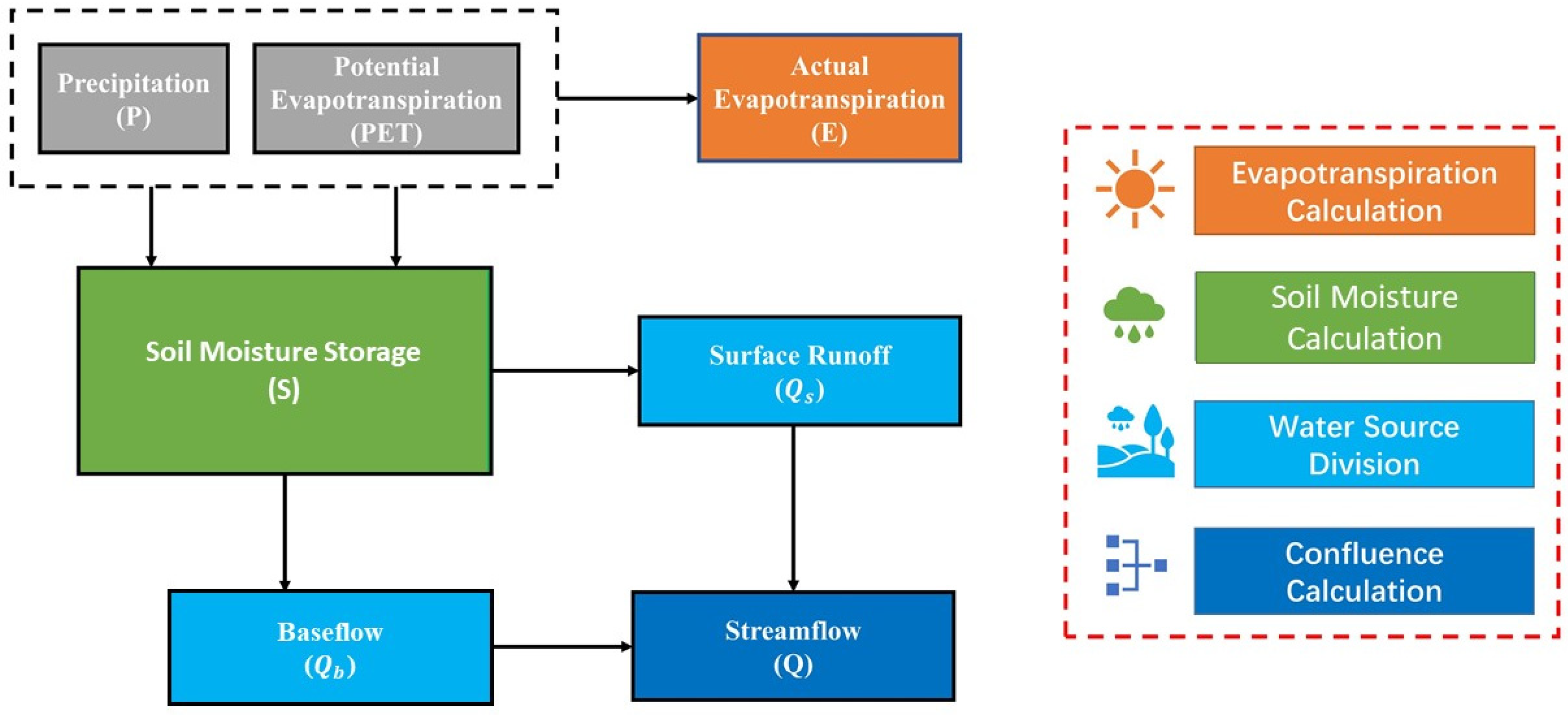
2.1. Monthly Water Balance Model

2.1.1. Three-Parameter Monthly Water Balance Model

The Wang Model (WM), a two-parameter monthly water balance model, is a conceptually simple monthly water balance model that can be used to estimate monthly flows using monthly rainfall and potential evapotranspiration data [49]. The WM model has been successfully applied to semi-arid and humid watersheds in China with only three parameters [50]. In comparison to other hydrological models such as SIMHYD, TANK, and SMAR, it not only has a more straightforward structure, fewer parameters, and greater flexibility, but it also performs well. Different components of the model are estimated using Equations (1)–(3).
E ( t ) = P E T ( t ) × S ( t ) S m a x                                      
Q s ( t ) = k s [ S ( t 1 ) S m a x ] P ( t )            
Q b ( t ) = k g × S ( t 1 )            
The variable E ( t ) is the actual monthly evaporation value of the catchment; P E T ( t ) is the monthly potential evapotranspiration value; P ( t ) is the monthly precipitation; t is the time; Q S ( t ) is the monthly surface runoff volume; S ( t ) is the monthly soil water content; Q b ( t ) is the monthly baseflow volume; S m a x is the maximum monthly soil water content of the watershed; k s is the runoff coefficient; k g is the baseflow coefficient.

2.1.2. Improved Three-Parameter Monthly Water Balance Model

This study develops an improved three-parameter monthly water balance model called the Chen Model (CM). The model is constructed as shown in Figure 1. According to the innovation of Xiong and Guo [39], the actual evaporation from the watershed is calculated using the Ol’dekop equation [51]. It can be considered as a conversion factor from evaporation dish observations to actual evaporation values, which is a hyperbolic t a n h ( ) function of the ratio of precipitation to evaporation dish observations. The t a n h ( x ) function for a given compression, x reflects the greater buffering and regulating capacity of watershed soils compared to air for hydrological phenomena or processes. Based on the monthly potential evapotranspiration values and monthly precipitation, the actual monthly evaporation values of the catchments were obtained using Equation (4) as follows:
E ( t ) = k × P E T ( t ) × t a n h ( P ( t ) P E T ( t ) )          
where k is the first parameter of the model to respond to the evaporation and precipitation changes.
If the entire catchment is treated as a reservoir, assuming that the monthly surface runoff is a hyperbolic t a n h ( ) function of the soil water content. The monthly surface runoff is obtained from the net soil water content of the month (i.e., the soil water content of the previous period plus the precipitation of the month minus the actual evaporation of the month) using Equation (5) as follows:
Q S ( t ) = ( S ( t 1 ) + P ( t ) E ( t ) ) × t a n   h ( S ( t 1 ) + P ( t ) E ( t ) S C )  
where S C is the second parameter of the model, which usually represents the maximum monthly soil water content of the entire watershed.
An exponential equation was utilized in the baseflow calculation (Equation (6)), but in the WM model, a linear equation was used. Because baseflow storage capacity is seldom equally distributed, a linear equation cannot accurately replicate the actual condition of baseflow. To solve the issue of continually changing groundwater storage capacity, the CM model mimics the unequal distribution of tension water by describing groundwater storage capacity distribution as a parabola, which can more precisely imitate the baseflow than the WM model. Compared to linear techniques, using exponential equations to model baseflow is more consistent with groundwater outflow.
Q b ( t ) = ( S ( t 1 ) + P ( t ) E ( t ) ) × e ( ( S ( t 1 ) + P ( t ) E ( t ) ) × ( d ) )          
The third parameter d of the model represents the baseflow coefficient.
The output value of the model is the total monthly runoff flow Q ( t ) (Equation (7)), and the entire catchment needs to meet the monthly water balance (Equation (8)) as follows:
Q ( t ) = Q S ( t ) + Q b ( t )        
S ( t ) S ( t 1 ) = P ( t ) E ( t ) Q ( t )    
According to the physical significance of the three parameters of this model, the range of values of the three parameters can be given, and the range applies to areas with different geographical features, with k from 0.5 to 1.5, SC from 100 to 2000, and d from 0.01 to 1.00.

2.1.3. Four-Parameter Monthly Water Balance Model

The four-parameter monthly water balance model (ABCD) is a conceptual hydrological model proposed by Thomas [37], which has been applied in several wet or semi-humid basins in China, with the same input data as the WM model and an additional groundwater content in the output data [15]. The water balance in a soil aquifer is represented by Equation (9).
P ( t ) E ( t ) Q S ( t ) Q b ( t ) = S ( t ) S ( t 1 )      
The two-state variables (effective water volume W ( t ) and possible evapotranspiration Y ( t ) in the ABCD model are calculated using Equations (10)–(12) as follows:
W ( t ) = S ( t 1 ) + P ( t ) = S ( t ) + E ( t ) + Q S ( t ) + Q b ( t )        
Y ( t ) = S ( t ) + E ( t )        
W ( t ) is related to Y ( t ) as a nonlinear function as follows:
Y ( t ) = W ( t ) + b 2 a ( W ( t ) + b 2 a ) 2 b W ( t ) a          
where a is the probability of forming runoff before the soil is fully saturated and takes a value in the range of (0, 1]; b is the upper limit of unsaturated aquifer storage capacity and takes a value in the range of (0, 1000]. The relationship between soil moisture content and potential evapotranspiration is given by Equation (13).
S ( t ) = Y ( t ) e x p ( P E T ( t ) b )              
The water balance equations of the model for the groundwater layer are as follows:
G ( t ) + G D ( t ) = G ( t 1 ) + Q b ( t )            
Q b ( t ) = c ( W ( t ) Y ( t ) )          
G D ( t ) = d G ( t )          
where G ( t ) is the amount of underground storage in the current month; G D ( t ) is the underground runoff; G ( t 1 ) is the amount of underground storage in the previous month; c is the proportion of the amount of groundwater recharged by the soil aquifer, taking the value range of (0, 1]; d is the rate of groundwater formation outflow, taking the value range of (0, 1].

2.2. Performance Indicators

The accuracy of satellite rainfall data was evaluated by percentage bias (Pbais), root mean square error (RMSE), and correlation coefficient (CC). In addition, the effect of the hydrological model runoff simulation was evaluated using the Nash efficiency coefficient (NSE) (Nash and Sutcliff, 1970 [52]) and percentage bias (Pbais). The performance indicators are given by Equations (17)–(20).
R M S E = i = 1 n ( P s i P o i ) 2 n
C C = i = 1 n ( P o i P o ¯ ) ( P s i P s ¯ ) i = 1 n ( P o i P o ¯ ) 2 i = 1 n ( P s i P s ¯ ) 2
N S E = 1 i = 1 n ( Q o b s t Q s i m t ) 2 i = 1 n ( Q o b s t Q o b s t ¯ ) 2            
P b a i s = 100 × i = 1 n Q i e s t i = 1 n Q i o b s i = 1 n Q i o b s          
where P o i is the observed rainfall; P s i satellite rainfall; Q o b s t is the observed runoff; Q s i m t is the simulated runoff.

2.3. Assessment of Impacts of Climate Change and Human Activities on Streamflow

2.3.1. The Budyko-Based Method

The elasticity factor approach based on the Budyko framework combines the Budyko model with a watershed water balance model, where human activities and climate change are the main factors affecting runoff changes [53]. Climate change is mainly characterized as changes in precipitation and potential evapotranspiration, and changes in coupled hydrothermal parameters and other effects are described as anthropogenic impacts for quantitative calculations [54]. In a closed catchment, its multi-year water balance is expressed as:
P = E + Q + Δ S
where P , E , and Q represent catchment precipitation, evaporation, and runoff, respectively; Δ S is the catchment water storage variable, which is negligible on a multi-year average scale.
According to the assumption of Budyko [55], the annual average actual evapotranspiration can be estimated from precipitation and potential evapotranspiration, i.e., E / P = F ( Φ ) , where Φ = P E T   / P , which describes the dryness of a region. The change in runoff due to climate change can be calculated by the method proposed by Milly and Dunne [56].
Δ Q c l i m = Q P Δ P + Q P E T Δ P E T
where Δ P and Δ P E T are the changes in precipitation and potential evapotranspiration, respectively; Q / P and ∂Q∂PET are the sensitivity coefficients of runoff to precipitation and potential evapotranspiration, respectively. The sensitivity coefficients of runoff to precipitation and potential evapotranspiration can be calculated from Equation (21) and the Budyko series of hydrothermal equations. When based on the Foucauldian formula [57], the sensitivity coefficient can be expressed as:
Q P = ( 1 + x w ) ( 1 / w ) x w   ( 1 + x w ) ( 1 / w 1 )
Q P E T = x ( w 1 )   ( 1 + x w ) ( 1 / w 1 ) 1
where w is a model parameter related to vegetation type, soil hydraulic properties, and topography terrain [58]. It can be calculated based on the annual average P , P E T , and Q of the basin.

2.3.2. Method of Separating Environment Variables

The hydrological time series (especially the streamflow time series) are generally divided into “natural phase” and “human-influenced phase” according to the change nodes, i.e., “base period” and “impact period”, depending on the degree of influence of human activities on the natural environment in the study area. Human activities and climate change have been the fundamental causes of the difference between the observed streamflow in the impact and base periods [46]. Human activities and climate change have not affected the observed streamflow series in the base period. The hydrological time series in the impact period is simulated using the enhanced three-parameter monthly water balance model with the streamflow data as the base period, while the observed streamflow series in the impact period derives from the combined influence of both. The difference between the simulated streamflow in the impact period and the measured streamflow in the base period is used to calculate the climate change component. In contrast, the difference between the simulated streamflow in the impact period and the measured streamflow in the same period is used to calculate the human activities component. The specific calculation formulas are as follows:
Δ R = R 1 R 0 = Δ R c l i m a t e + Δ R h u m a n
Δ R c l i m a t e = R R 0
Δ R h u m a n = R 1 R
η c l i m a t e = Δ R c l i m a t e Δ R × 100 %
η h u m a n = Δ R h u m a n Δ R × 100 %
where Δ R is the total streamflow change; R 1 is the measured streamflow during the impact period; R 0 is the measured streamflow during the base period; R is the simulated streamflow during the impact period; Δ R c l i m a t e is the impact value of climate change on streamflow; Δ R h u m a n is the impact value of human activities on streamflow; η c l i m a t e and η h u m a n are the contribution rates of climate change and human activities on streamflow change, respectively.

3. Study Area and Data Sources
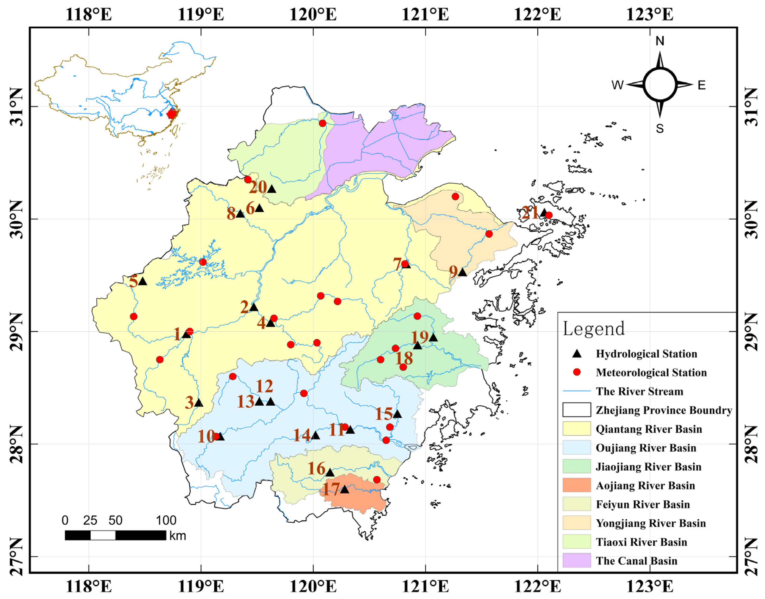
3.1. Study Area

Zhejiang Province lies in the southeastern section of China’s mainland, bordering the East China Sea, a humid and rainy zone with an average annual precipitation of more than 1600 mm and an average annual precipitation day between 140 and 180 days. Zhejiang’s geography trends from southwest to northeast, with high points in the southwest and low points in the northeast. The southwest is mostly mountain ranges with elevations of more than 1000 meters; the central part is hilly and catchment with an altitude of about 50–500 meters, and the northeast is plain with an altitude less than 10 meters, with the mountainous hills accounting for 70.4 percent of the province’s land area. Many rivers are formed by the abundance of water and the steep terrain. From north to south, Zhejiang Province has major water systems, including the Tiaoxi (TX) River Basin, Canal Basin, Qiantangjiang (QTJ) River Basin, Yongjiang (YJ) River Basin, Jiaojiang (JJ) River Basin, Oujiang (OJ) River Basin, Feiyunjiang (FYJ) River Basin, Aojiang (AJ) River Basin, Zhoushan Island (ZSI) River Basin (Figure 2), as well as a slew of tiny rivers that run into the sea and neighboring provinces on their own. A large plain formed by rivers, lakes, and shallow sea deposits exists in northern Zhejiang and coastal areas, and regional rivers and lakes are joined to build a dense water network, establishing a unique river network water system known as “Jiangnan Water Town”.

3.2. Data Sources

Streamflow data from 21 hydrological stations in Zhejiang Province were utilized as measured runoff data in this study, and the essential information for each hydrological station can be seen in Table 1. The China Meteorological Science Data Sharing Service (http://data.cma.cn, accessed on 12 May 2020) provided daily precipitation data, evaporation dish measurements, and the average temperature at meteorological stations in the watershed. The Thiessen polygon technique was used to calculate the watershed’s monthly surface rainfall.
The APHRODITE was created by the Japan Meteorological Agency (JMA) Research Foundation and utilized to collect satellite rainfall data for this study. APHRODITE gathered rainfall station measurements from around Asia and created gridded daily precipitation data with high precision [59]. The spatial resolution of the 1951–2007 precipitation reanalysis data for Central Asia is 0.25° × 0.25°. (V1101). In 2018, the same technique was used to develop an extended update (V1101EX_R1) covering 2008–2015 for diagnosing climate change and associated hydrological investigations (V1101).

4. Results

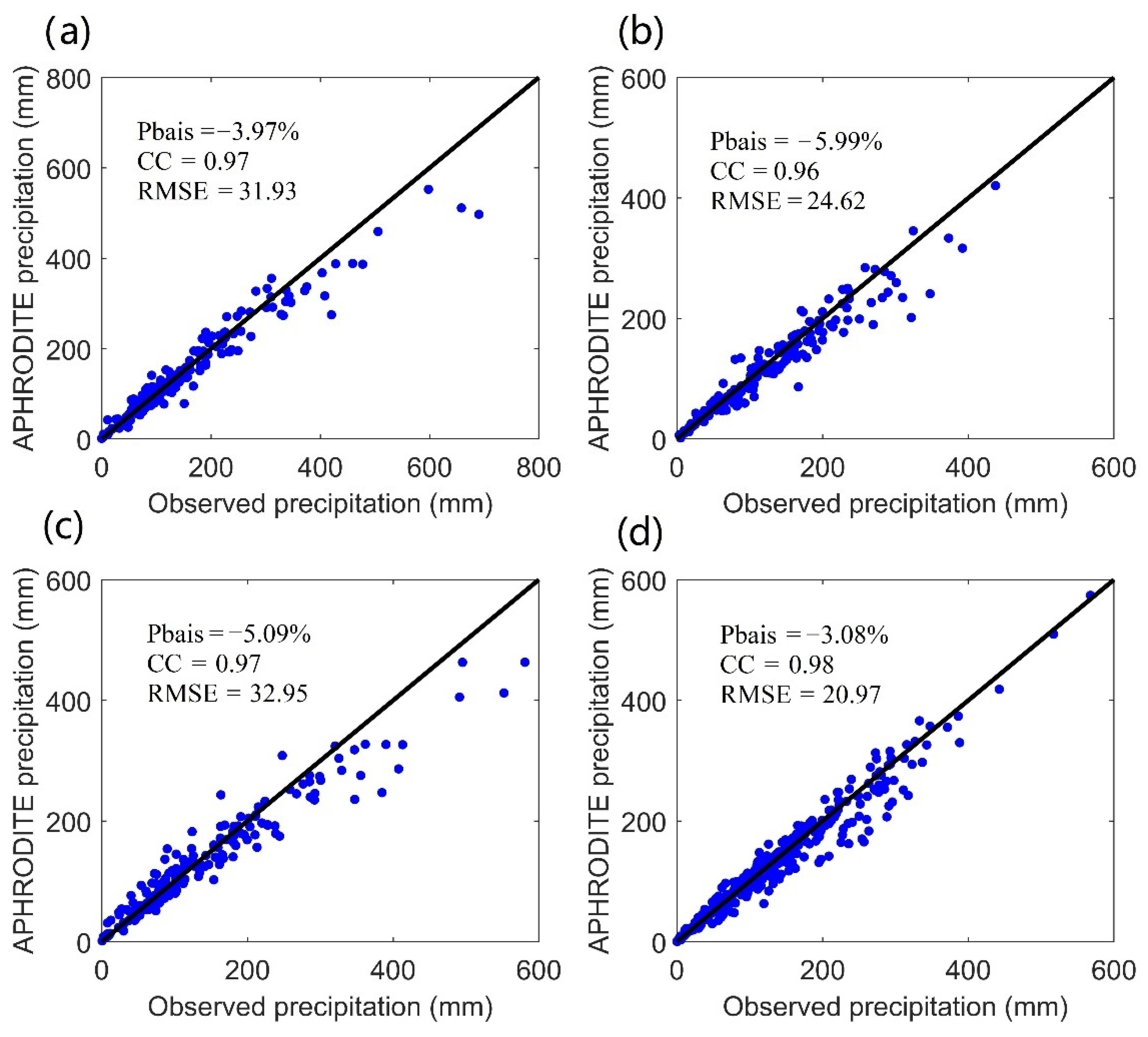
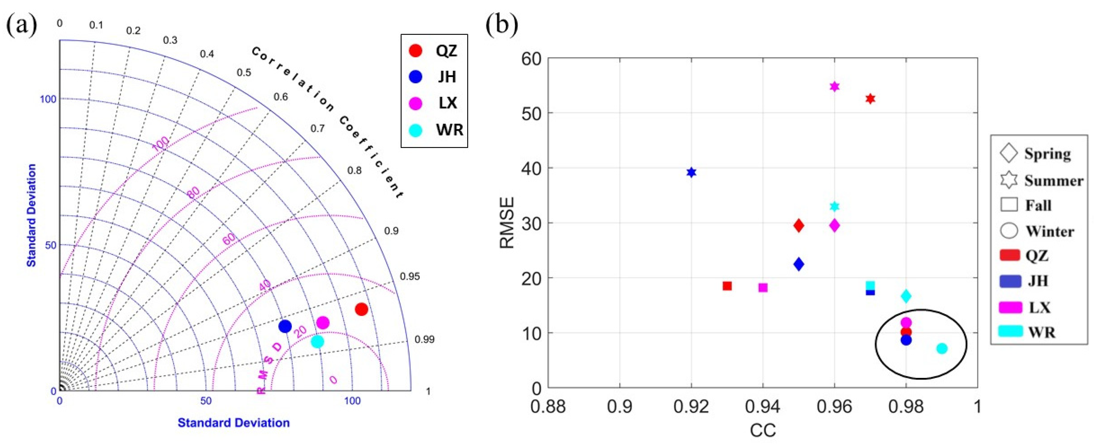
4.1. Assessment of APHRODITE Rainfall Product

Daily rainfall measurements from eight meteorological stations in the QTJ River basin from 1981 to 1995, as well as four meteorological stations in the OJ River basin from 1971 to 1998, were used to test the accuracy of APHRODITE rainfall products at the station scale in this study. The raster data of APHRODITE co-located with the observed rainfall stations were used for comparative analysis, and the results are the average of the comparison results of each station in each catchment. The scatter plots of the surface rainfall on the monthly time scale compared with the measured rainfall data at the rainfall stations are shown in Figure 3. The Pbais between APHRODITE satellite and measured rainfall at the monthly scale between the four catchments is 3.97%, −5.99%, −5.09%, and −3.08%, respectively, while the CC values are 0.97, 0.96, 0.97, and 0.98, and the RMSE values are 31.93, 24.62, 32.95, and 20.97. As a result, the APHRODITE satellite rainfall products offer excellent monthly accuracy.
Taylor diagrams at monthly scales for the catchments are given in Figure 4a to visualize the accuracy of satellite rainfall products at different scales and catchments. The length of its radius reflects the amount of change in the overall standard deviation, the angular relationship with the vertical coordinate represents the correlation coefficient, and the length from the observation point represents the error in Taylor diagrams. As a result, using the Taylor diagram helps to indicate how different precipitation products differ from recorded precipitation data at ground rainfall stations. The closer the simulated value’s geographic distribution is to the observed value, the shorter the simulated value’s distance from the observation point. Over diverse watersheds, the Taylor diagram displays the degree of superiority and inferiority of the APHRODITE satellite product estimations. At the watershed scale, as shown in Figure 4a, the WR station is closer to the observation point in the Taylor diagram, and the accuracy of the three sites (QZ, JH, and LX) within the QTJ River watershed is similar. As a result, the accuracy of APHRODITE satellite rainfall products on the OJ River basin is slightly greater than that of the QTJ River basin. The greater catchment area has a better hydrological model simulation performance, according to Table 1. The accuracy of APHRODITE satellite rainfall products is much greater in winter than in other seasons and somewhat less applicable in summer than in other seasons, as illustrated in Figure 4b. At the same time, the watershed scale provides a broader range of applications at the WR station.

4.2. Simulation Analysis of Monthly Water Balance Model

This study’s examination of the monthly water balance model’s simulation results is separated into two parts: (1) actual rainfall data from two watersheds (four catchments) were used to compare the simulation results of the three-parameter monthly water balance (CM) model with those of the WM and ABCD models; (2) APHRODITE precipitation data were used as the input to the hydrological model, and the CM, WM, and ABCD models for eight watersheds (21 catchments in total) in the Zhejiang Province.

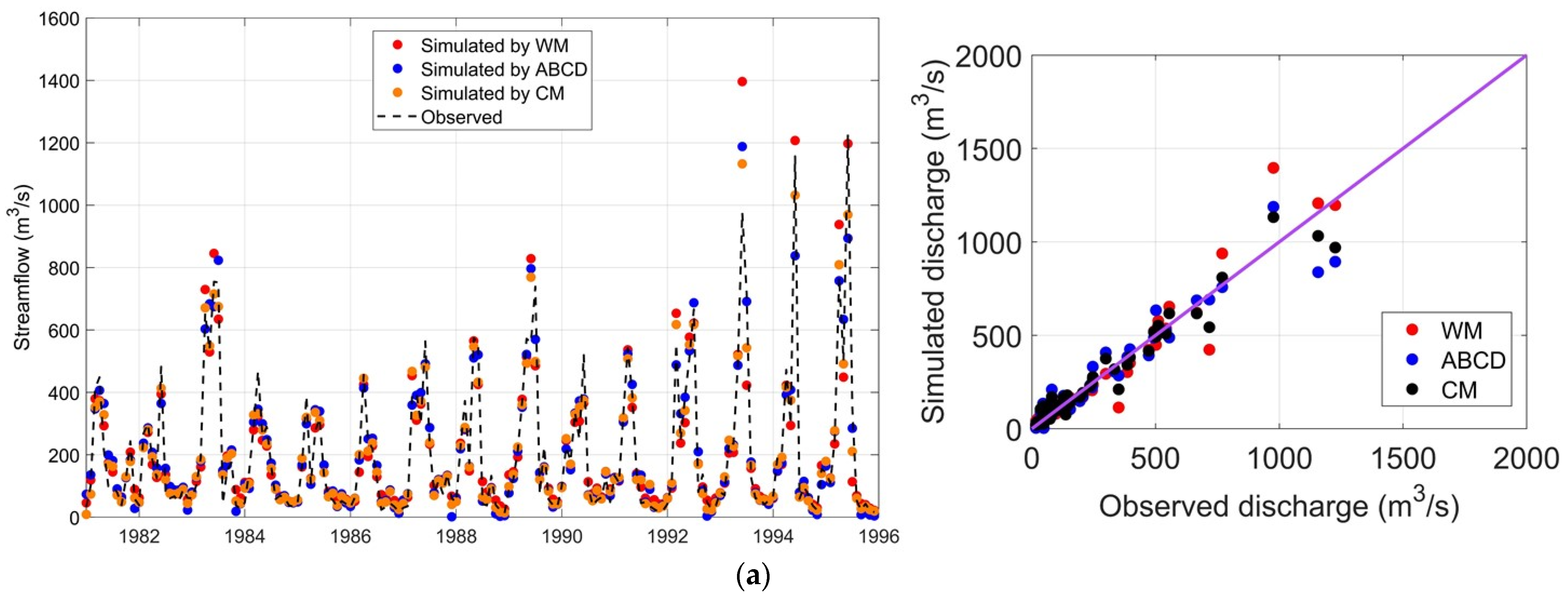
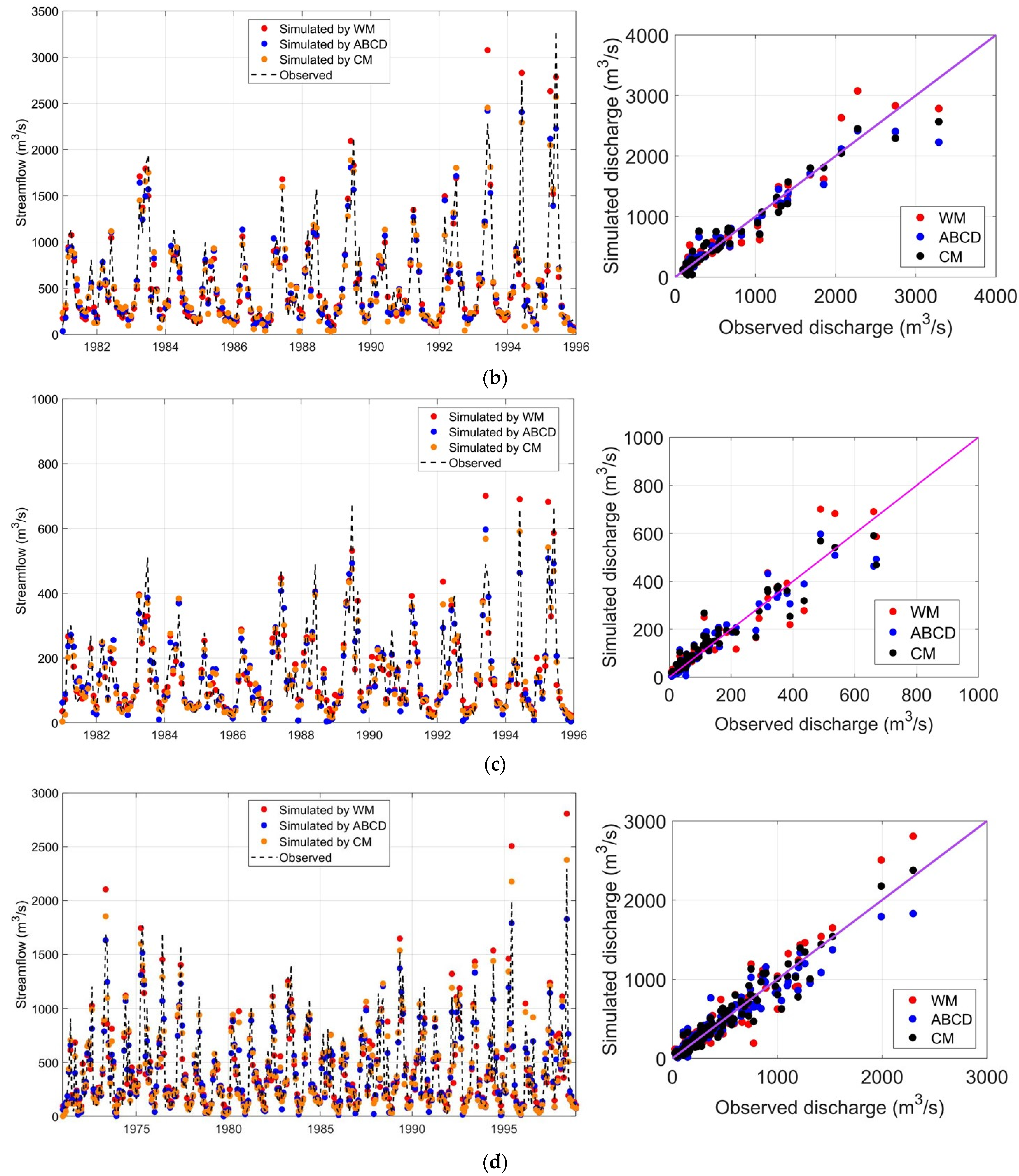
4.2.1. Simulation Results Using the Observed Rainfall

The WM, ABCD, and CM models were used to maximize the values of each model parameter in four catchments of the QTJ and OJ River basins. The NSE value based on simulated and measured streamflow was selected as the objective function for obtaining the optimal model parameters. A genetic algorithm-based solution approach is used to search for the optimal parameter set. Table 2 shows the parameter values for three hydrological models, and Table 3 shows the monthly streamflow simulation accuracy comparison for each model over the calibration and validation period. Table 2 and Table 3 show that the established water balance models in each catchment have great simulation accuracy, with the NSE values of the CM model over the validation period above 0.9 and substantially exceeding the simulation results of the WM and ABCD models. The Pbais of the WM model simulations are all positive, showing that the model is overestimated, but the percentage deviations of the CM model in each catchment are both positive and negative. The absolute numbers are regulated by 5%, allowing for proper water balance. Figure 5 depicts the simulated hydrological processes of each model in each catchment, as well as the simulated measured scatter plots. The simulation results of the CM model are closer to the actual hydrological process than the WM and ABCD models, as seen in the above figure, and the simulated and observed scatter spots are closer to the 1:1 line. The simulation ability of the three models for high flows is relatively close, but the CM model performs better in the simulation of low flows, and the simulation of the baseflow through the exponential equation is more consistent with the hydrological processes in the semi-humid and semi-arid regions of southern China.

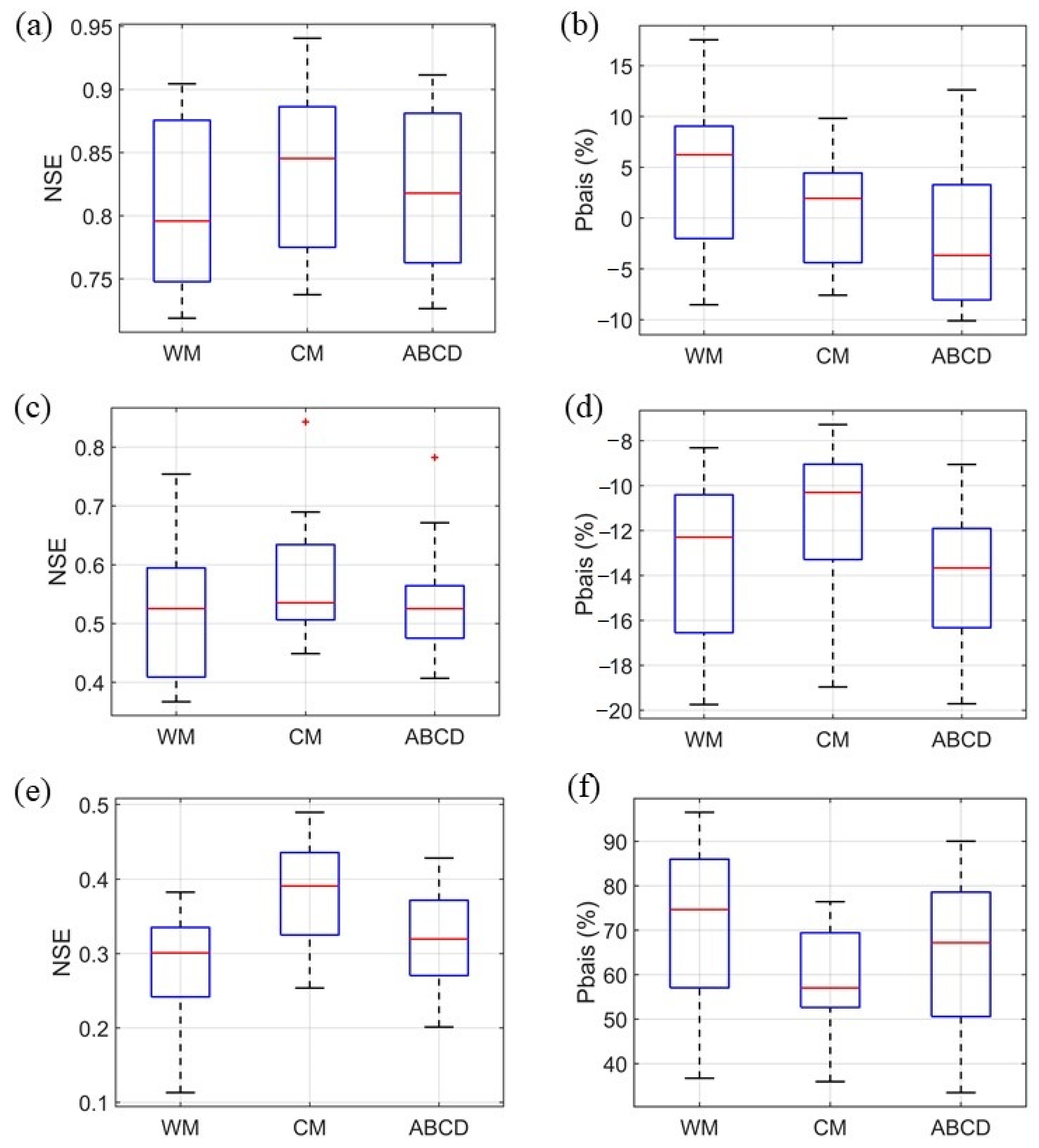
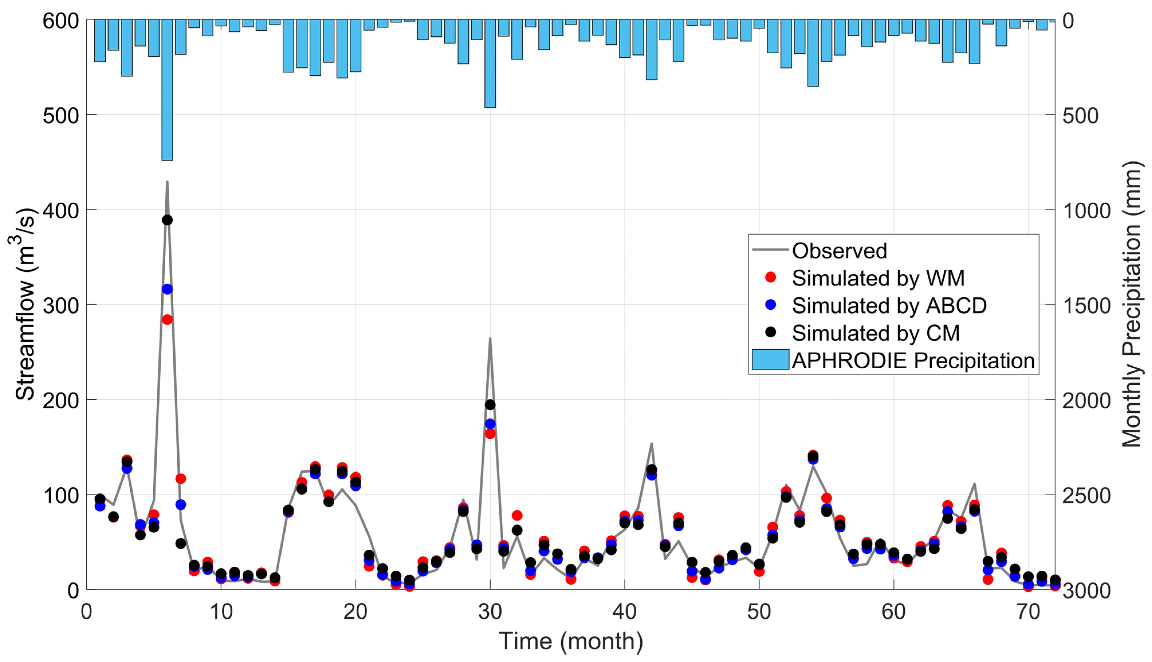
4.2.2. Simulation Results Using the APHRODITE Rainfall

The WM, ABCD, and CM models were applied to the QTJ River Basin (QZ, LX, ZG, JH, ZX, XF, SZ, and QSD stations), YJ River Basin (NXK station), OJ River Basin (LQ, WR, JJK, SB, BY, and SZ stations), FYJ River Basin (XK station), AJ River Basin (DT station), JJ River Basin (BZA and SD stations), TX River Basin (QDC station) and ZSI River Basin (CCL station), and the model NSE and Pbais for the calibration and validation period are shown in Table 4. The results show that the simulation accuracy of the established water balance models for each catchment is high, the NSE for each catchment during the calibration and validation period is greater than 0.7, the absolute values of Pbais are within 15%, and each model can satisfy the water balance using APHRODITE rainfall as the model input. The average NSE for the CM model validation period is about 0.85, whereas the average NSE values for the WM and ABCD models are 0.79 and 0.82, respectively. On the other hand, the Pbais value for the CM model in the validation period, on the other hand, is closer to 0 and less than 5%, suggesting that the model matches the monthly water balance within each watershed, showing that the CM model has suitable application in Zhejiang Province’s basins.
The streamflow above the 75th percentile is defined as peak flow, while that below the 25th percentile is considered as low flow. The peak flow and low flow simulation performance indicators for each model are shown in Figure 6. The three models are relatively close in their ability to simulate high flows, and this can be attributed to their reasonably accurate calculations for both actual evaporation and soil water content. All models show a good low-flow simulation capability due to the higher accuracy of precipitation input used in these models. It is known from the previous section that APHRODITE precipitation product is more applicable in winter than in other seasons and that low flows of hydrological processes tend to occur in winter. However, the CM simulated low flow is better than the other two models in terms of NSE and Pbais values. The reason for this is that both WM and ABCD models use linear equations to simulate the receding process, while CM uses exponential expressions that are more consistent with the actual baseflow process.
To illustrate this phenomenon more closely, Figure 7 depicts the simulation results of hydrological processes in the LQ catchment of the OJ River basin in order to better observe the simulation of hydrological processes by each model. All models can accurately mimic the monthly runoff process for the LQ catchment, and the simulated values of the peak streamflow have high consistency with observations. At the same time, the CM model’s simulation of the hydrological process is more accurate than the WM and ABCD models, particularly in terms of peak and minimum values, and the peak-shaped process is closer to the experimental process. According to the results in Table 3 and Table 4, the rain gauge product provides better streamflow estimates than the APHRODITE product for the three given models. However, the difference in simulation performance between the two is not significant, and both provide a better representation of the basic hydrologic processes in the catchment.
This part splits the 21 catchments into three ranges by comparing the NSE and Pbais values of the model within various catchment regions (see Figure 8) to explore the application of the three-parameter monthly water balance model at the geographical scale: ① catchment area < 1000 km2; ② 1000 km2 < catchment area < 5000 km2; ③ catchment area > 5000 km2. When the catchment area exceeds 5000 km2, the model’s simulation capability becomes critical. Using the NSE as an example, the CM model’s average NSE value is greater than 0.9, and the absolute value of the mean Pbais is less than 1% when the catchment area is greater than 5000 km2. The reason for this phenomenon is that the bias of APHRODITE rainfall product is smaller in watersheds with large catchment areas, while small catchment areas are more challenging for the simulation capability of the ensemble hydrological model. It should be noted that the accuracy of each model simulation result is slightly poor owing to the effect of rainfall data or human activities in different watersheds. The following study will investigate the impact of climate change and human activities on the change in watershed runoff in-depth to solve this problem.

4.2.3. Impacts of Climate Change and Human Activities on Streamflow Changes

The hydrological cycle in the basin has changed due to the dual effect of climate change and human activity, causing the rainfall-runoff process in the basin to deviate from the historical hydrological process. In this changing environment, the first step in the hydrological study is to determine if the basin’s rainfall-runoff mechanism fits the stationarity assumption. The Mann–Kendall test (Mann, 1945 [60]) was used for each watershed in Zhejiang Province to assess the abrupt change points in the runoff series: under the same coordinate system, two statistical curves, UF and UB, as well as the upper and lower critical lines. If UF and UB overlap within the upper and lower crucial lines, the year when the junction occurs is the mutation year. The significance level α = 0.05 was chosen, and the corresponding critical value U 0.05 = ± 1.96 . The Mann–Kendall test curves of annual runoff at different time scales for 21 catchments in 8 River basins are shown in Figure 9.
Based on the findings of the streamflow abrupt change study, a Budyko-based and hydrological model technique was used to evaluate the influence of climate change and human activities on streamflow. The research period was divided into two halves of different environmental factors: the base period and the impact period. The CM model was used to investigate the causes of streamflow changes in each watershed in Zhejiang Province. Table 5 shows the results of the two techniques’ calculations, and the two methods’ estimations of streamflow variations resulting from climate change and human activities are primarily comparable. The contribution of climate change and human activities to streamflow changes using the hydrological model method in each watershed is shown in Figure 10. It can be observed that climatic change dominates streamflow variations in 18 of the 21 catchments, while human activities contributed to those variations in the other three. Furthermore, the results are more consistent throughout multiple catchments in each watershed. In the OJ River basin, all stations show a decrease in streamflow due to human activities, but an increase in streamflow caused by climate change. Climate change contributes 51.39 percent to 87.39 percent in the QTJ River basin, with only declining streamflow at SZ station being a direct result of it. Except for the NXK watershed, climate change dominance spans from 60.97 percent to 80.74 percent throughout the OJ River basin. The contribution rates of human activities impacting yearly streamflow fluctuations in the JJ River basin (BZA and SD catchments) were 60.51 percent and −91.99 percent, respectively.
Climate change and human activities impact the geographical distribution of yearly runoff from watersheds in Zhejiang Province (see Figure 11). Climate change has a greater impact on the province’s watersheds than human activity. However, human activities have a greater effect on the eastern coastal areas than climate change, which might be supported by land-use changes (rural to urban) or other changes in those watersheds as shown to be impacted by human activities.

5. Discussions

It is worth pointing out that rainfall data are crucial for creating accurate models of hydrological processes as it is the main input to the models. As all the research regions are mesoscale watersheds with a maximum streamflow propagation time of less than 1 day from the uppermost section of the watershed control area to the streamflow station, a monthly temporal scale was employed to analyze the spatial distribution of satellite rainfall products. Additionally, studies [61,62] have indicated that watersheds with quicker production and confluence times are less affected by the spatial distribution of rainfall. The method for comparing satellite precipitation products with observation precipitation is another crucial issue that has to be considered. Thiessen polygon, a spatial interpolation technique, is not a reasonable way to compare product correctness [63]. As a result, the scale of the meteorological station was chosen for comparison. The APHRODITE dataset is the only high-resolution, long-term gridded information on land rainfall covering the entire Asian region, and the rainfall estimates are highly accurate at the monthly temporal scale [64,65]. Rainfall data from APHRODITE was selected as the model input because the hydrological model utilized in this work operates on a monthly scale. The monthly water balance model is a conceptual hydrological model based on the principle of monthly water balance [66,67], which has the advantages of simple structure and fewer parameters. In this study, a three-parameter monthly water balance model is modified, and the baseflow calculation was carried out using an exponential equation. The three models are fairly comparable in terms of their ability to simulate high flows, but the CM model is more effective at simulating low flows, and simulating baseflow using an exponential equation is more in line with the hydrological processes in the semi-humid and semi-arid regions of southern China. Further research is needed on the applicability of the model in other regions, such as arid regions. On the other hand, the baseflow simulation capability of this hydrological model cannot be evaluated due to the limitation of the accurate baseflow, but the improved model is improved in terms of the simulation capability of low flows.
When using this hydrological model to simulate watershed responses under changing environments, more climatic factors and human activity factors (e.g., land use type and vegetation cover conditions) are not considered in relation to runoff changes due to the limitations of the model characteristics. Different types of human activities may have different effects on runoff changes, so further research can be conducted in the future to separate the effects of different types of human activities on runoff changes. Furthermore, many studies [68,69,70] on attribution analysis are founded on the premise that human activity and climate change are independent of one another. However, in actual watersheds, human activity and climate change interact with one another, so future research is expected to continue to investigate how to conduct attribution analysis in these situations.

6. Conclusions

In this study, the accuracy of APHRODITE rainfall data is examined and studied, which uses eight river systems in Zhejiang Province as research objects. The research area’s runoff process is simulated and tested using an enhanced three-parameter monthly water balance model. Finally, by isolating environmental factors, the impacts of climate change and human activities on runoff changes were assessed. The key findings are stated below:
(1) The APHRODITE satellite rainfall products offer great accuracy on a monthly scale, with a CC mean of more than 0.96 and an average absolute Pbais of less than 5%. In addition, the accuracy of APHRODITE rainfall data is higher in the winter than in the other seasons and slightly less so in the summer.
(2) Three monthly water balance models offer good simulation accuracy and hydrological process inversion. Furthermore, the average NSE utilizing the CM model is greater than 0.9, indicating that the water balance may be accurately met. The CM model mimics the hydrological process better than the WM and ABCD models, particularly in the modeling of low flow processes, which is closer to the experimental process.
(3) In their estimations of streamflow variations as impacted by climate change and human activities, the Budyko-based and hydrological model methodologies are typically compatible. Climate change is the primary driver of streamflow variations in 18 of Zhejiang Province’s 21 watersheds, while human activities are the primary driver in the other three. Climate change has a more significant impact on most river systems than human activities, although human activities have a greater impact on eastern coastal areas than climate change.

Author Contributions

Conceptualization, H.C. and Y.-P.X.; methodology, S.H.; software, Y.G.; validation, J.X.; formal analysis, H.N.; investigation, H.C.; resources, S.H.; data curation, R.S.V.T.; writing—original draft preparation, H.C.; writing—review and editing, R.S.V.T.; visualization, Y.-P.X.; supervision, Y.-P.X.; project administration, S.H.; funding acquisition, H.C. All authors have read and agreed to the published version of the manuscript.

Funding

This research was funded by the Zhejiang Key Research and Development Plan, grant number 2021C03017; the Major Project of the Natural Science Foundation of Zhejiang, grant number LZ20E090001; and the Zhejiang Provincial Natural Science Foundation, grant number LZJWY22E090007.

Data Availability Statement

The daily precipitation data, evaporation dish observations, and average temperature at meteorological stations in the basin are obtained from the China Meteorological Science Data Sharing Service (http://data.cma.cn, accessed on 10 January 2020). The APHRODITE dataset is available from https://www.chikyu.ac.jp/precip/ (accessed on 12 May 2020).

Acknowledgments

The authors would like to thank Zhejiang Provincial Hydrological Management Center for providing hydrologic data used in this study.

Conflicts of Interest

The authors declare no conflict of interest.

References

  1. Dey, P.; Mishra, A. Separating the impacts of climate change and human activities on streamflow: A review of methodologies and critical assumptions. J. Hydrol. 2017, 548, 278–290. [Google Scholar] [CrossRef]
  2. Yan, T.; Bai, J.; Lee, Z.Y.A.; Shen, Z. SWAT-simulated streamflow responses to climate variability and human activities in the Miyun Reservoir Basin by considering streamflow components. Sustainability 2018, 10, 941. [Google Scholar] [CrossRef]
  3. Wu, J.; Miao, C.; Zhang, X.; Yang, T.; Duan, Q. Detecting the quantitative hydrological response to changes in climate and human activities. Sci. Total Environ. 2017, 586, 328–337. [Google Scholar] [CrossRef] [PubMed]
  4. Grill, G.; Lehner, B.; Thieme, M.; Geenen, B.; Tickner, D.; Antonelli, F.; Babu, S.; Borrelli, P.; Cheng, L.; Crochetiere, H.; et al. Mapping the world’s free-flowing rivers. Nature 2019, 569, 215–221. [Google Scholar] [CrossRef] [PubMed]
  5. Yu, C.; Huang, X.; Chen, H.; Godfray, H.C.J.; Wright, J.S.; Hall, J.W.; Gong, P.; Ni, S.; Qiao, S.; Huang, G.; et al. Managing nitrogen to restore water quality in China. Nature 2019, 567, 516–520. [Google Scholar] [CrossRef]
  6. Tang, Q. Global change hydrology: Terrestrial water cycle and global change. Sci. China Earth Sci. 2020, 63, 459–462. [Google Scholar] [CrossRef]
  7. Wang, X.B.; He, K.N.; Dong, Z. Effects of climate change and human activities on runoff in the Beichuan River Basin in the northeastern Tibetan Plateau, China. Catena 2019, 176, 81–93. [Google Scholar] [CrossRef]
  8. Zhang, H.; Meng, C.; Wang, Y.; Li, M. Comprehensive evaluation of the effects of climate change and land use and land cover change variables on runoff and sediment discharge. Sci. Total Environ. 2020, 702, 134401. [Google Scholar] [CrossRef]
  9. Liu, Y.; Hu, X.; Wu, F.; Chen, B.; Liu, Y.; Yang, S.; Weng, Z. Quantitative analysis of climate change impact on Zhangye City’s economy based on the perspective of surface runoff. Ecol. Indic. 2019, 105, 645–654. [Google Scholar] [CrossRef]
  10. Kong, D.; Miao, C.; Wu, J.; Duan, Q. Impact assessment of climate change and human activities on net runoff in the Yellow River Basin from 1951 to 2012. Ecol. Eng. 2016, 91, 566–573. [Google Scholar] [CrossRef]
  11. Deng, C.; Liu, P.; Wang, D.; Wang, W. Temporal variation and scaling of parameters for a monthly hydrologic model. J. Hydrol. 2018, 558, 290–300. [Google Scholar] [CrossRef]
  12. Meng, S.; Xie, X.; Yu, X. Tracing temporal changes of model parameters in rainfall runoff modeling via a real-time data assimilation. Water 2016, 8, 19. [Google Scholar] [CrossRef]
  13. Pathiraja, S.; Marshall, L.; Sharma, A.; Moradkhani, H. Hydrologic modeling in dynamic catchments: A data assimilation approach. Water Resour. Res. 2016, 52, 3350–3372. [Google Scholar] [CrossRef]
  14. Wallner, M.; Haberlandt, U. Non-stationary hydrological model parameters: A framework based on SOM-B. Hydrol. Process. 2015, 29, 3145–3161. [Google Scholar] [CrossRef]
  15. Wang, D.; Tang, Y. A one-parameter Budyko model for water balance captures emergent behavior in darwinian hydrologic models. Geophys. Res. Lett. 2014, 41, 4569–4577. [Google Scholar] [CrossRef]
  16. Feng, M.; Liu, P.; Guo, S.; Shi, L.; Deng, C.; Ming, B. Deriving adaptive operating rules of hydropower reservoirs using time-varying parameters generated by the EnKF. Water Resour. Res. 2017, 53, 6885–6907. [Google Scholar] [CrossRef]
  17. Troin, M.; Martel, J.; Arsenault, R.; Brissette, F. Large-sample study of uncertainty of hydrological model components over North America. J. Hydrol. 2022, 609, 127766. [Google Scholar] [CrossRef]
  18. Rocha, J.; Carvalho-Santos, C.; Diogo, P.; Beça, P.; Keizer, J.J.; Nunes, J.P. Impacts of climate change on reservoir water availability, quality and irrigation needs in a water scarce Mediterranean region (southern Portugal). Sci. Total Environ. 2020, 736, 39477. [Google Scholar] [CrossRef]
  19. Arsenault, R.; Brissette, F. Analysis of continuous streamflow regionalization methods within a virtual setting. Hydrolog. Sci. J. 2016, 61, 2680–2693. [Google Scholar] [CrossRef]
  20. Troin, M.; Arsenault, R.; Wood, A.W.; Brissette, F.; Martel, J.-L. Generating ensemble streamflow forecasts: A review of methods and approaches over the past 40 years. Water Resour. Res. 2021, 57, e2020WR028392. [Google Scholar] [CrossRef]
  21. Mockler, E.M.; O’Loughlin, F.E.; Bruen, M. Understanding hydrological flow paths in conceptual catchment models using uncertainty and sensitivity analysis. Comput. Geosci. 2016, 90, 66–77. [Google Scholar] [CrossRef]
  22. Wang, F.; Huang, G.H.; Fan, Y.; Li, Y.P. Development of a disaggregated multi-level factorial hydrologic data assimilation model. J. Hydrol. 2022, 610, 127802. [Google Scholar] [CrossRef]
  23. Wan, Y.; Chen, J.; Xu, C.Y.; Xie, P.; Qi, W.; Li, D.; Zhang, S. Performance dependence of multi-model combination methods on hydrological model calibration strategy and ensemble size. J. Hydrol. 2021, 603, 127065. [Google Scholar] [CrossRef]
  24. Darbandsari, P.; Coulibaly, P. Inter-comparison of lumped hydrological models in data-scarce watersheds using different precipitation forcing data sets: Case study of Northern Ontario, Canada. J. Hydrol. 2020, 31, 100730. [Google Scholar] [CrossRef]
  25. Khaniya, M.; Tachikawa, Y.; Ichikawa, Y.; Yorozu, K. Impact of assimilating dam outflow measurements to update distributed hydrological model states: Localization for improving ensemble Kalman filter performance. J. Hydrol. 2022, 608, 127651. [Google Scholar] [CrossRef]
  26. Remondi, F.; Kirchner, J.W.; Burlando, P.; Fatichi, S. Water flux tracking with a distributed hydrological model to quantify controls on the spatio-temporal variability of transit time distributions. Water Resour. Res. 2018, 54, 3081–3099. [Google Scholar] [CrossRef]
  27. Bai, P.; Liu, X.; Liang, K.; Liu, C. Comparison of performance of twelve monthly water balance models in different climatic catchments of China. J. Hydrol. 2015, 529, 1030–1040. [Google Scholar] [CrossRef]
  28. Yao, C.; Zhang, K.; Yu, Z.; Li, Z.; Li, Q. Improving the flood prediction capability of the Xinanjiang model in ungauged nested catchments by coupling it with the geomorphologic instantaneous unit hydrograph. J. Hydrol. 2014, 517, 1035–1048. [Google Scholar] [CrossRef]
  29. Cheng, S.; Cheng, L.; Liu, P.; Zhang, L.; Xu, C.; Xiong, L.; Xia, J. Evaluation of baseflow modelling structure in monthly water balance models using 443 Australian catchments. J. Hydrol. 2020, 591, 125572. [Google Scholar] [CrossRef]
  30. Bastola, S.; Murphy, C.; Sweeney, J. The role of hydrological modelling uncertainties in climate change impact assessments of Irish river catchments. Adv. Water Resour. 2011, 34, 562–576. [Google Scholar] [CrossRef]
  31. Hamel, P.; Guswa, A.J.; Sahl, J.; Zhang, L.; Abebe, A. Predicting dry-season flows with a monthly rainfall-runoff model: Performance for gauged and ungauged catchments. Hydrol. Process. 2017, 31, 3844–3858. [Google Scholar] [CrossRef]
  32. Thornthwaite, C.W. An approach toward a rational classification of Climate. Geogr. Rev. 1948, 38, 55–94. [Google Scholar] [CrossRef]
  33. Thornthwaite, C.W.; Mather, J.R. The Water Balance; Laboratory of Climatology, Drexel Institute of Technology: Centerton, NJ, USA, 1955; Volume 8, pp. 1–104. [Google Scholar]
  34. Shafii, M.; Craig, J.R.; Macrae, M.L.; English, M.C.; Schiff, S.L.; Van Cappellen, P.; Basu, N.B. Can improved flow partitioning in hydrologic models increase biogeochemical predictability? Water Resour. Res. 2019, 55, 2939–2960. [Google Scholar] [CrossRef]
  35. Khatami, S.; Peel, M.C.; Peterson, T.J.; Western, A.W. Equifinality and flux mapping: A new approach to model evaluation and process representation under uncertainty. Water Resour. Res. 2019, 55, 8922–8941. [Google Scholar] [CrossRef]
  36. Gupta, H.V.; Wagener, T.; Liu, Y. Reconciling theory with observations: Elements of a diagnostic approach to model evaluation. Hydrol. Process. 2008, 22, 3802–3813. [Google Scholar] [CrossRef]
  37. Thomas, H.A. Improved Methods for National Water Assessment; Center for Integrated Data Analytics Wisconsin Science Center: Washington, DC, USA, 1981. [Google Scholar]
  38. Makhlouf, Z.; Michel, C. A two-parameter monthly water balance model for French watersheds. J. Hydrol. 1994, 162, 299–318. [Google Scholar] [CrossRef]
  39. Xiong, L.; Guo, S. A two-parameter monthly water balance model and its application. J. Hydrol. 1999, 216, 111–123. [Google Scholar] [CrossRef]
  40. Yang, L.; Feng, Q.; Yin, Z.; Wen, X.; Si, J.; Li, C.; Deo, R.C. Identifying separate impacts of climate and land use/cover change on hydrological processes in upper stream of Heihe River, Northwest China. Hydrol. Process. 2017, 31, 1100–1112. [Google Scholar] [CrossRef]
  41. Ning, T.; Li, Z.; Liu, W. Separating the impacts of climate change and land surface alteration on runoff reduction in the Jing River catchment of China. Catena 2016, 147, 80–86. [Google Scholar] [CrossRef]
  42. Omer, A.; Ma, Z.G.; Zheng, Z.Y.; Saleem, F. Natural and anthropogenic influences on the recent droughts in Yellow River Basin, China. Sci. Total Environ. 2020, 704, 135428. [Google Scholar] [CrossRef]
  43. Hero, M.; Booij, M.J.; Hoekstra, A.Y. Hydrological response to future land-use change and climate change in a tropical catchment. Hydrolog. Sci. J. 2018, 63, 1368–1385. [Google Scholar] [CrossRef]
  44. Zhang, J.; Gao, G.; Fu, B.; Zhang, L. Explanation of climate and human impacts on sediment discharge change in Darwinian hydrology: Derivation of a differential equation. J. Hydrol. 2018, 559, 827–834. [Google Scholar] [CrossRef]
  45. Li, B.; Yu, Z.; Liang, Z.; Song, K. Effects of climate variations and human activities on runoff in the Zoige Alpine Wetland in the eastern edge of the Tibetan Plateau. J. Hydrol. Eng. 2014, 19, 1026–1035. [Google Scholar] [CrossRef]
  46. Zhang, L.; Nan, Z.; Wang, W.; Ren, D.; Zhao, Y.; Wu, X. Separating climate change and human contributions to variations in streamflow and its components using eight time-trend methods. Hydrol. Process. 2019, 33, 383–394. [Google Scholar] [CrossRef]
  47. Zhao, J.; Wang, D.; Yang, H.; Sivapalan, M. Unifying catchment water balance models for different time scales through the maximum entropy production principle. Water Resour. Res. 2016, 52, 7503–7512. [Google Scholar] [CrossRef]
  48. Getirana, A.C.V.; Espinoza, J.C.V.; Ronchail, J.; Filho, O.C.R. Assessment of different precipitation datasets and their impacts on the water balance of the Negro River basin. J. Hydrol. 2011, 404, 304–322. [Google Scholar] [CrossRef]
  49. Dinku, T.; Chidzambwa, S.; Ceccato, P.; Connor, S.J.; Ropelewski, C.F. Validation of High-resolution satellite rainfall products over complex terrain. Int. J. Remote Sens. 2008, 29, 4097–4110. [Google Scholar] [CrossRef]
  50. Wang, G.Q.; Zhang, J.Y.; Jin, J.L.; Liu, Y.L.; He, R.M.; Bao, Z.X.; Liu, C.S.; Li, Y. Regional calibration of a water balance model for estimating stream flow in ungauged areas of the Yellow River Basin. Quat. Int. 2013, 336, 65–72. [Google Scholar] [CrossRef]
  51. Wilffried, B. Evaporation into the Atmosphere: Theory, History and Application; Cornell University Press: Ithaca, NY, USA, 1992; pp. 241–244. [Google Scholar]
  52. Nash, J.E.; Sutcliffe, J.V. River flow forecasting through conceptual models part I-A discussion of principles. J. Hydrol. 1970, 10, 282–290. [Google Scholar] [CrossRef]
  53. Jiang, C.; Xiong, L.; Wang, D.; Liu, P.; Guo, S.; Xu, C.Y. Separating the impacts of climate change and human activities on runoff using the Budyko-type equations with time-varying parameters. J. Hydrol. 2015, 522, 326–338. [Google Scholar] [CrossRef]
  54. Zhang, S.; Yang, H.; Yang, D.; Jayawardena, A.W. Quantifying the effect of vegetation change on the regional water balance within the Budyko framework. Geophys. Res. Lett. 2016, 43, 1140–1148. [Google Scholar] [CrossRef]
  55. Budyko, M.I. Climate and Life; Academic Press: San Diego, CA, USA, 1974. [Google Scholar]
  56. Milly, P.C.; Dunne, K.A. Macroscale water fluxes 2. Water and energy supply control of their inter-annual variability. Water Resour. Res. 2002, 38, 241–249. [Google Scholar] [CrossRef]
  57. Liang, W.; Bai, D.; Wang, F.; Fu, B.; Yan, J.; Wang, S. Quantifying the impacts of climate change and ecological restoration on streamflow changes based on a Budyko hydrological model in China’s Loess Plateau. Water Resour. Res. 2015, 51, 6500–6519. [Google Scholar] [CrossRef]
  58. Yang, H.; Yang, D.; Hu, Q. An error analysis of the Budyko hypothesis for assessing the contribution of climate change to runoff. Water Resour. Res. 2014, 50, 9620–9629. [Google Scholar] [CrossRef]
  59. Umer, M.; Gabriel, H.F.; Haider, S.; Nusrat, A.; Shahid, M. Application of precipitation products for flood modeling of transboundary river basin: A case study of Jhelum Basin. Theor. Appl. Climatol. 2021, 143, 989–1004. [Google Scholar] [CrossRef]
  60. Mann, H.B. Nonparametric tests against trend. Econometrica 1945, 13, 245–259. [Google Scholar] [CrossRef]
  61. Sapriza-Azuri, G.; Jodar, J.; Navarro, V.; Jan Slooten, L.; Carrera, J.; Gupta, H.V. Impacts of rainfall spatial variability on hydrogeological response. Water Resour. Res. 2015, 51, 1300–1314. [Google Scholar] [CrossRef]
  62. Younger, P.M.; Freer, J.E.; Beven, K.J. Detecting the effects of spatial variability of rainfall on hydrological modelling within an uncertainty analysis framework. Hydrol. Processes 2009, 23, 1988–2003. [Google Scholar] [CrossRef]
  63. Faiz, M.A.; Zhang, Y.; Baig, F.; Wrzesinski, D.; Naz, F. Identification and inter-comparison of appropriate long-term precipitation datasets using decision tree model and statistical matrix over China. Int. J. Climatol. 2021, 41, 5003–5021. [Google Scholar] [CrossRef]
  64. Li, Z.; Yang, D.W.; Hong, Y. Multi-scale evaluation of high-resolution multi-sensor blended global precipitation products over the Yangtze River. J. Hydrol. 2013, 500, 157–169. [Google Scholar] [CrossRef]
  65. Jiang, S.; Ren, L.; Yang, H.; Yong, B.; Yang, X.; Fei, Y.; Ma, M. Comprehensive evaluation of multi-satellite precipitation products with a dense rain gauge network and optimally merging their simulated hydrological flows using the Bayesian model averaging method. J. Hydrol. 2012, 452–453, 213–225. [Google Scholar] [CrossRef]
  66. Nasseri, M.; Zahraie, B.; Ajami, N.K.; Solomatine, D.P. Monthly water balance modeling: Probabilistic, possibilistic and hybrid methods for model combination and ensemble simulation. J. Hydrol. 2014, 511, 675–691. [Google Scholar] [CrossRef]
  67. Liu, W.; Engel, B.A.; Feng, Q. Modelling the hydrological responses of green roofs under different substrate designs and rainfall characteristics using a simple water balance model. J. Hydrol. 2021, 602, 126786. [Google Scholar] [CrossRef]
  68. Chang, J.; Zhang, H.; Wang, Y.; Zhu, Y. Assessing the impact of climate variability and human activity to streamflow variation. Hydrol. Earth Syst. Sci. 2016, 20, 1547–1560. [Google Scholar] [CrossRef]
  69. Greve, P.; Gudmundsson, L.; Orlowsky, B.; Seneviratne, S.I. A two-parameter Budyko function to represent conditions under which evapotranspiration exceeds precipitation. Hydrol. Earth Syst. Sci. 2019, 20, 2195–2205. [Google Scholar] [CrossRef]
  70. Zhou, S.; Yu, B.; Huang, Y.; Wang, G. The complementary relationship and generation of the Budyko functions. Geophys. Res. Lett. 2015, 42, 1781–1790. [Google Scholar] [CrossRef] [Green Version]
Figure 1. Conceptual diagram of the three-parameter monthly water balance hydrological model.
Remotesensing 14 04411 g001
Figure 2. Location of the study area showing different basins and hydrometeorological stations.
Remotesensing 14 04411 g002
Figure 3. Scatter plot of (a) QZ, (b) JH, (c) LX, and (d) WR stations APHRODITE rainfall products compared to the measured rainfall.
Remotesensing 14 04411 g003
Figure 4. (a) Taylor diagram of monthly scale observations and APHRODITE precipitation products and (b) comparison of the accuracy of observations and APHRODITE precipitation products on seasonal scales.
Remotesensing 14 04411 g004
Figure 5. (a) Simulated and measured monthly runoff processes at QZ station. (b) Simulated and measured monthly runoff processes at JH station. (c) Simulated and measured monthly runoff processes at LX station. (d) Simulated and measured monthly runoff processes at WR station.
Remotesensing 14 04411 g005aRemotesensing 14 04411 g005b
Figure 6. Simulation performance indicators box diagram in (a,b) all streamflow, (c,d) 75th percentile, and (e,f) 25th percentile for each model validation period.
Remotesensing 14 04411 g006
Figure 7. Comparison of simulated and measured monthly runoff at LQ Station.
Remotesensing 14 04411 g007
Figure 8. Correspondence between NSE and Pbais values of CM model at different watershed areas.
Remotesensing 14 04411 g008
Figure 9. Mann–Kendall test for annual streamflow in each sub-basin and year of abrupt change from (a) QZ, (b) LX, (c) ZG, (d) JH, (e) ZZ, (f) XF, (g) SZ, (h) QSD, (i) NXK, (j) LQ, (k) WZ, (l) JJK, (m) SB, (n) BY, (o) SZ, (p) XK, (q) DT, (r) BZA, (s) SD, (t) QDC, and (u) CCL.
Remotesensing 14 04411 g009
Figure 10. Contribution of annual runoff to human activities and climate change using hydrological model method in each sub-basin.
Remotesensing 14 04411 g010
Figure 11. Map of the dominant distribution of annual streamflow in each river system by human activities and climate change.
Remotesensing 14 04411 g011
Table 1. Information on hydrological stations in the study area.
Station NumberStation NameRiver SystemPeriod of RecordCalibration PeriodValidation PeriodDrainage Area (km2)
1Quzhou (QZ)Qiantangjiang1981–19951981–1990 1991–1995 5545
2Lanxi (LX)Qiantangjiang1981–19951981–1990 1991–1995 18,204
3Zhonggeng (ZG)Qiantangjiang1979–19931979–1988 1989–1993 610
4Jinhua (JH)Qiantangjiang1981–19951981–1990 1991–1995 5920
5Zhongzhou (ZZ)Qiantangjiang1975–19941975–1987 1988–1994 94
6Xufan (XF)Qiantangjiang1964–19971964–1986 1987–1997 62
7Shengzhou (SZ)Qiantangjiang2000–20072000–2004 2005–2007 2291
8Qinshandian (QSD)Qiantangjiang1970–19941970–1986 1987–1994 1329
9Nanxikou (NXK)Yongjiang1970–19901970–1983 1984–1990 126
10Longquan (LQ)Oujiang1987–20031987–1997 1998–2003 1469
11Weiren (WZ)Oujiang1971–19981971–1988 1989–1998 13,500
12Jingjukou (JJK)Oujiang1968–20051968–1992 1993–2005 1880
13Shangbao (SB)Oujiang1968–19931968–1984 1985–1993 499
14Baiyan (BY)Oujiang1981–20051981–1997 1998–2005 3172
15Shizhu (SZ)Oujiang2000–20102000–20062007–2010 1359
16Xuekou (XK)Feiyunjiang2000–20122000–2008 2009–2012 1932
17Daitou (DT)Aojiang1991–20101991–2004 2005–2010 338
18Baizhiao (BZA)Jiaojiao1961–20121961–1995 1996–2012 2475
19Shaduan (SD)Jiaojiao1980–20121980–2001 2002–2012 1482
20Qiaodongcun (QDC)Tiaoxi1961–19981961–1985 1986–1998 242
21Changchunling (CCL)Zhoushan Island2002–20082002–2005 2006–2008 3.9
Table 2. Parameter values of three models for each watershed.
StationWM ModelABCD ModelCM Model
SmaxkskgabcdkSCd
QZ298.040.900.0030.87210.810.130.040.87710.460.09
LX538.030.650.0110.81205.910.370.181.071040.790.10
JH296.920.710.0010.91223.250.250.120.93540.190.05
WR333.790.990.0010.85213.510.010.990.70416.380.46
Smax = maximum monthly soil water content of the watershed, ks = runoff coefficient, kg = baseflow coefficient; a = probability of forming runoff before the soil is fully saturated, b = upper limit of unsaturated aquifer storage capacity, c = proportion of the amount of groundwater recharged by the soil aquifer, d = rate of groundwater formation outflow; k = evaporation and precipitation changes, SC = maximum monthly soil water content of the entire watershed, d = baseflow coefficient.
Table 3. Comparison of the three models’ simulation results for each watershed using observed rainfall data.
StationWM ModelABCD ModelCM Model
CalibrationValidationCalibrationValidationCalibrationValidation
NSEPbais(%)NSEPbais(%)NSEPbais(%)NSEPbais(%)NSEPbais(%)NSEPbais(%)
QZ0.902.000.912.110.912.850.92−1.350.92−0.030.96−1.29
LX0.880.310.923.460.89−0.050.93−1.760.88−0.120.94−2.28
JH0.892.110.876.930.831.390.892.080.85−0.090.903.20
WR0.882.270.873.060.86−2.610.91−3.010.91−0.620.930.40
Table 4. Comparison of three models simulation results for each watershed using the APHRODITE rainfall.
StationWM ModelABCD ModelCM Model
CalibrationValidationCalibrationValidationCalibrationValidation
NSEPbais(%)NSEPbais(%)NSEPbais(%)NSEPbais(%)NSEPbais(%)NSEPbais(%)
QZ0.869.260.90−3.570.89−0.290.90−10.110.893.190.92−5.78
LX0.84−1.050.89−8.530.86−0.470.91−7.020.851.650.92−3.68
ZG0.866.310.88−1.720.90−0.100.87−8.020.873.660.90−3.71
JH0.743.210.896.640.75−1.160.915.260.7610.960.892.79
ZZ0.807.960.88−2.900.83−0.190.88−8.840.824.260.89−4.50
XF0.749.050.798.050.79−0.190.772.620.740.270.782.93
SZ0.693.820.73−6.970.77−0.220.75−4.760.71−4.740.752.49
QSD0.827.390.7512.960.85−0.420.825.540.810.950.855.52
NXK0.769.650.75−1.590.76−0.390.75−4.780.785.200.76−5.79
LQ0.934.670.850.220.93−0.200.90−3.670.924.860.940.63
WR0.866.130.885.290.87−0.280.89−0.550.875.150.895.06
JJK0.875.130.866.220.86−0.050.871.770.874.500.874.25
SB0.8114.380.839.150.85−0.510.85−4.190.855.400.851.94
BY0.803.620.8010.940.81−0.830.825.610.801.270.834.97
SZ0.7615.460.769.010.83−0.540.821.690.862.260.853.59
XK0.729.350.778.630.79−1.430.801.390.78−6.250.81−4.35
DT0.760.390.80−6.910.75−4.950.75−9.720.85−0.660.81−6.03
BZA0.7711.400.7710.000.76−0.440.777.290.785.540.787.31
SD0.754.490.7217.550.70−0.070.7312.620.743.960.749.81
QDC0.7411.850.732.240.80−0.720.75−8.160.785.550.74−3.23
CCL0.6717.810.728.890.83−0.710.77−8.800.823.040.77−7.59
Table 5. The two techniques’ estimations of streamflow variations resulting from climate change and human activities.
River BasinStationBydyko−BasedCM
wηclimate (%)ηhuman (%)ηclimate (%)ηhuman (%)
QTJQZ0.9369.6530.3573.8226.18
LX1.2268.1531.8579.8920.11
ZG1.0760.5939.4173.7326.27
JH1.1772.98−27.0261.35−38.65
ZZ0.8160.8939.1161.7538.25
XF1.4659.85−40.1551.39−48.61
SZ1.34−78.78−21.22−87.39−12.61
QSD0.9966.25−33.7558.09−41.91
YJNXK0.5022.21−77.7925.72−74.28
OJLQ0.8495.61−4.3960.97−39.03
WR0.8797.38−2.6275.83−24.27
JJK1.1285.92−14.0876.41−23.59
SB0.77−57.52−42.48−79.31−20.69
BY0.7079.54−20.4575.93−24.07
SZ0.7157.68−42.3280.74−19.26
FYJXK0.6260.06−39.9490.96−9.04
AJDT0.2469.7630.2498.921.08
JJBZA1.05−31.7668.24−39.4960.51
SD1.18−36.74−63.26−8.01−91.99
TXQDC0.9151.7448.2676.6723.33
ZSICCL1.7071.6228.3877.6422.36
Positive indicates an increase in streamflow, negative notes a decrease in streamflow.
Publisher’s Note: MDPI stays neutral with regard to jurisdictional claims in published maps and institutional affiliations.

