Article

Generalized LiDAR Intensity Normalization and Its Positive Impact on Geometric and Learning-Based Lane Marking Detection

Lyles School of Civil Engineering, Purdue University, West Lafayette, IN 47907, USA
*
Author to whom correspondence should be addressed.
Remote Sens. 2022, 14(17), 4393; https://doi.org/10.3390/rs14174393
Submission received: 21 July 2022 / Revised: 26 August 2022 / Accepted: 31 August 2022 / Published: 3 September 2022

Abstract

:
Light Detection and Ranging (LiDAR) data collected by mobile mapping systems (MMS) have been utilized to detect lane markings through intensity-based approaches. As LiDAR data continue to be used for lane marking extraction, greater emphasis is being placed on enhancing the utility of the intensity values. Typically, intensity correction/normalization approaches are conducted prior to lane marking extraction. The goal of intensity correction is to adjust the intensity values of a LiDAR unit using geometric scanning parameters (i.e., range or incidence angle). Intensity normalization aims at adjusting the intensity readings of a LiDAR unit based on the assumption that intensity values across laser beams/LiDAR units/MMS should be similar for the same object. As MMS technology develops, correcting/normalizing intensity values across different LiDAR units on the same system and/or different MMS is necessary for lane marking extraction. This study proposes a generalized correction/normalization approach for handling single-beam/multi-beam LiDAR scanners onboard single or multiple MMS. The generalized approach is developed while considering the intensity values of asphalt and concrete pavement. For a performance evaluation of the proposed approach, geometric/morphological and deep/transfer-learning-based lane marking extraction with and without intensity correction/normalization is conducted. The evaluation shows that the proposed approach improves the performance of lane marking extraction (e.g., the F1-score of a U-net model can change from 0.1% to 86.2%).

Graphical Abstract

1. Introduction

Lane markings such as skip or solid lines are essential for delineating transportation corridors, managing traffic activities, and road safety analysis. They exhibit higher reflectivity than nearby road surfaces since retroreflective glass beads are incorporated into lane marking paint. This contrast will be pronounced in Light Detection and Ranging (LiDAR) data, which encompass both position and reflectivity information in the form of point clouds with intensity values. LiDAR scanners continuously emit laser pulses and evaluate ranges through the time lapse between the signal emission and reception of its reflection. The intensity of the received return, which is usually digitized as an 8-bit integer (0–255), depends on the reflective properties of the objects in the waveband of the used pulse as well as the intersection geometry between the laser beam and object surface. According to the number of laser rods in a LiDAR unit, it can be categorized either as a single-beam or multi-beam unit. Recently, LiDAR data captured by mobile mapping systems (MMS) have been utilized to detect lane markings through intensity-based approaches [1,2,3,4,5,6]. As LiDAR data continue to be utilized for lane marking extraction, greater emphasis is being placed on enhancing the utility of intensity values (i.e., by reducing variability in the intensity values for returns from a given object). Strategies for the intensity enhancement of LiDAR data can be divided into four levels [7]:
  • Level 0—no intensity modification;
  • Level 1—intensity correction: adjust the intensity values of a LiDAR unit using geometric scanning parameters (e.g., range and/or incidence angle);
  • Level 2—intensity normalization: normalize the intensity readings of a LiDAR unit based on the assumption that intensity values across laser beams/LiDAR units/MMS should be similar for the same object;
  • Level 3—intensity calibration: rectify the intensity values of a LiDAR unit based on known reflectance readings derived from a reference target.
Typically, level 1 or 2 (intensity correction/normalization) approaches are conducted prior to lane marking extraction. For instance, Jaakkola et al. [1] performed intensity correction before lane marking extraction. They fitted a polynomial curve using intensity readings and scanning ranges. Then, the fitted function was used to reduce intensity variation. Thereafter, processed point clouds were utilized for lane marking extraction. Guan et al. [2] conducted intensity correction to reduce intensity variation caused by scanning ranges for lane marking extraction. First, they detected road surfaces from original point clouds using curbstone points. Extracted road surface point clouds were then rasterized into intensity images using inverse distance weighting (IDW) interpolation [8]. More specifically, the intensity weight for each point was determined by its scanning range. Finally, the intensity images were utilized for lane marking extraction. Teo and Yu [3] corrected LiDAR intensity values using empirical polynomials for lane marking extraction. They partitioned road surface point clouds and then applied polynomial fitting to intensity and range values. The obtained polynomials were used to reduce the impact of scanning ranges on intensity readings. Finally, corrected point clouds were classified into two categories: lane marking and pavement. Cheng et al. [4] proposed an incident-angle-based approach for intensity correction. They assumed that the intensity values of a lane marking should be a function of the incident angle since the scanning range and material of a pavement marker are almost the same. Accordingly, the relationship between the intensity readings and incident angles of lane markings was estimated through linear regression modeling. With the derived model, the intensity values of road surface point clouds could be corrected for lane marking extraction.
Although the above approaches have enhanced the utility of intensity values, the used parameters or assumptions are inconsistent. Hence, Levinson and Thrun [5,6] proposed an unsupervised normalization approach for a multi-beam LiDAR sensor which solely depends on intensity readings. It assumes that the same objects’ intensity values across laser beams must be similar. They segmented a road surface point cloud to generate an intensity normalization look-up table (LUT), as is discussed in more detail later in this manuscript. Based on the LUT, the intensity of point clouds captured by the same LiDAR unit can be normalized.
Given the continuous development of MMS technologies and changes in road characteristics, more challenges are encountered during intensity enhancement:
  • Recently, several MMS equipped with multiple LiDAR units (e.g., single and/or multi-beam scanners from different manufacturers) have been developed [9]. Figure 1 shows sample point clouds and corresponding intensity histograms (along the same road surface) captured by Riegl VUX 1HA [10] (single-beam), Z+F Profiler 9012 [11] (single-beam), and Velodyne HDL-32E [12] (multi-beam) LiDAR units. For the same road region, the Riegl VUX 1HA intensity readings range from 70 to 140, while those from Z+F Profiler 9012 are in the 0 to 120 range. The Velodyne HDL-32E intensity values, on the other hand, are between 0 and 30. Thus, a generalized framework that can handle different LiDAR units onboard the same or different systems is required for lane marking extraction.
  • Asphalt and concrete are the most common pavement types. According to Kashani et al. [7], asphalt and concrete pavement regions show distinctly different intensity values (i.e., most asphalt intensity readings are lower than concrete ones). Thus, intensity readings from asphalt/concrete pavement regions should be considered while developing a generalized normalization framework.
In summary, most intensity correction/normalization approaches focus on one LiDAR unit (intra-sensor). However, as MMS technology develops, correcting/normalizing intensity values across different LiDAR units on the same system and/or different MMS is necessary for lane marking extraction. Moreover, most of the previous studies have only been performed for asphalt pavement regions. Considering the different intensity values for various pavement types, the impact of asphalt and concrete pavement on correction/normalization approaches needs to be investigated. In addition to geometric/morphological approaches, recent advancements in machine learning and deep learning technologies have stimulated the development of learning-based lane marking detection [13,14,15], which could be potentially adopted for autonomous vehicles (AV) [16]. However, the impact of intensity normalization on geometric/morphological and deep/transfer-learning-based lane marking extraction remains an open problem. This paper addresses these challenges by developing a generalized framework to correct/normalize intensity values for lane marking extraction. The main contributions of this study can be summarized as follows:
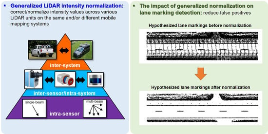
  • A generalized intensity correction/normalization approach (as illustrated in Figure 2) is proposed for:
    • A single-beam or multi-beam LiDAR scanner (intra-sensor).
    • LiDAR units onboard a mobile mapping system (inter-sensor/intra-system).
    • Point clouds from several mobile mapping systems (inter-system).
  • The generalized correction/normalization approach is developed while considering the impact of observed intensity values along asphalt and concrete pavement regions.
  • To evaluate the performance of the proposed approach, geometric/morphological and deep-learning-based lane marking extraction with and without intensity correction/normalization are conducted.
  • To further evaluate the proposed approach, transfer learning is applied to a deep learning model for handling datasets from different MMS. The performance of a fine-tuned model with and without intensity correction/normalization is also compared.
  • Considering asphalt/concrete pavement and different patterns of lane markings (such as dotted, dash, or solid lines), 168-mile-long LiDAR data collected by two MMS on three highways are used for comprehensive performance evaluation.
The remainder of this paper is organized as follows: Section 2 introduces the used MMS and LiDAR data. Section 3 presents the proposed generalized correction/normalization framework and adopted geometric and learning-based lane marking extraction strategies. The experiment results are reported in Section 4, followed by Section 5, which discusses the key findings. Finally, the conclusions and scope for future work are summarized in Section 6.

2. Data Acquisition Systems and Dataset Description

2.1. Mobile Mapping Systems

According to the research objectives, this study requires more than one MMS equipped with various LiDAR units (e.g., single- or multi-beam LiDAR scanners from different manufacturers). Thus, this study employs two different MMS: Purdue wheel-based mobile mapping system—ultra high accuracy (PWMMS-UHA) and Purdue wheel-based mobile mapping system—high accuracy (PWMMS-HA). The PWMMS-UHA, as displayed in Figure 3a, is equipped with two single-beam LiDAR scanners: one Riegl VUX 1HA and one Z+F Profiler 9012. These single-beam scanners deliver a 360° horizontal field of view (FOV). The Riegl VUX-1HA can scan approximately 1,000,000 points per second [10]. Similarly, the Z+F profiler 9012 can scan more than 1,000,000 points per second [11]. In addition, two rear-facing FLIR Flea2 FireWire cameras are installed on the PWMMS-UHA. Both cameras have a maximum image resolution of 5.0 MP and are synchronized to capture images at a rate of 1 frame per 0.75 s per camera. All sensors are directly georeferenced by a NovAtel ProPak6 GNSS/INS system [17]. This GNSS/INS system is based on ISA-100C near navigation grade IMU with a measurement rate of 200 Hz.
The PWMMS-HA, as shown in Figure 3b, includes four multi-beam LiDAR scanners: three Velodyne HDL-32Es and one Velodyne VLP-16 Hi-Res [18]. The HDL-32E consists of 32 radially oriented laser rangefinders aligned vertically from −30.67° to +10.67°; thus, the total vertical FOV is 41.34°. The VLP-16 Hi-Res has 16 radially oriented laser rangefinders with a vertical FOV from −10° to +10°. In addition, these four LiDAR scanners can rotate to achieve a 360° horizontal FOV. The point capture rates for HDL-32E and VLP-16 Hi-Res are 700,000 points per second [12] and 300,000 points per second [18], respectively. Three FLIR Grasshopper3 9.1MP GigE cameras are also mounted on the PWMMS-HA: two forward-facing and one rear-facing. The cameras are synchronized to capture images at a rate of 1 frame per second per camera. The above equipment is directly georeferenced by an Applanix POS LV 220 GNSS/INS unit [19]. The GNSS collection rate is 20 Hz, and the measurement rate of the IMU is 200 Hz [19]. Table 1 lists the specifications of the LiDAR units onboard the PWMMS-UHA and PWMMS-HA.

2.2. Study Site and Dataset Description

To investigate the impact of asphalt and concrete pavement, three highways in the United States—US-41/52 (Lafayette, IN to Hammond, IN), US-231 (Lafayette, IN to Crawfordsville, IN), and I-65/865/465 (Lafayette, IN to Indianapolis, IN)—were selected in this study. Figure 4 shows the study sites and vehicle trajectory, where locations i–vi are local concrete and asphalt regions for developing and testing the proposed intensity correction/normalization approach, as is discussed in Section 4.1 and Section 4.2. In addition, RGB images capturing locations i–vi taken by one of the cameras onboard the PWMMS-HA are presented in Figure 4. Both MMS could capture two lanes (including left, center, and right edge lines) with a single pass. Table 2 lists the specifications of the acquired datasets. The average local point spacing (LPS) [20] of the point clouds captured by the Riegl VUX 1HA, Z+F Profiler 9012, HDL-32E, and VLP-16 Hi-Res are 3.5 cm, 3.5 cm, 5.0 cm, and 7.5 cm, respectively. Combining the point clouds captured by all the LiDAR units, the average LPSprovided by the PWMMS-UHA and PWMMS-HA systems are 2.5 cm and 3.8 cm, respectively.

3. Methodology

This section starts by describing the proposed generalized intensity correction/normalization approach. Next, the adopted geometric/morphological and learning-based lane marking extraction strategies are introduced. Finally, metrics for evaluating the lane marking extraction performance are discussed.

3.1. Generalized Intensity Normalization

To effectively handle single-beam/multi-beam LiDAR scanners onboard single or multiple mobile mapping systems, a generalized intensity normalization framework is proposed. The proposed framework has three steps: intra-sensor, inter-sensor/intra-system, and inter-system, as depicted in Figure 2.

3.1.1. Intra-Sensor Intensity Correction—Single-Beam LiDAR

For a single-beam LiDAR unit, a range-based intensity correction approach [3] is adopted in this study. The conceptual basis of this approach is removing the dependency of observed intensity values on scanning ranges. For a road surface point cloud scanned from a 2D LiDAR at a given height, the incident angle is a function of the scanning range; therefore, using the scanning range implicitly considers the incident angle. Starting with segmenting a local area along the road surface (50 to 100 m long region), a polynomial function is fitted using the intensity values and their respective ranges of the LiDAR points within that region. The fitted polynomial function f ( r ) is used to derive corrected intensity values, which are independent of the scanning range, as can be seen in Equation (1). In the equation, a r is the original intensity, a r ^ is the corrected intensity, and r denotes the range. This approach solely relies on the scanning ranges, i.e., it does not require target deployment.
a r ^ = a r f ( r )

3.1.2. Intra-Sensor Intensity Normalization—Multi-Beam LiDAR

For a multi-beam LiDAR unit, a laser-beam-based intensity normalization approach [5,6] is adopted. This approach assumes that the normalized value of a given intensity reading from a particular beam is the conditional expectation of the intensity values observed by other beams. In this section, we use a 32-beam LiDAR unit that records 8-bit intensity values (e.g., Velodyne HDL-32E) as an example to illustrate the approach. First, a local area along the road surface (50 to 100 m long region) is segmented and gridded using 2D cells along the XY plane. For each point in the local area, its laser beam ID b and intensity value a are recorded as a tuple ( b , a ) , where b [ 0 ,   1 ,   2 , ,   31 ] and a [ 0 ,   1 ,   2 , ,   255 ] . For a unique pair ( b , a ) , all cells containing such pair are identified. The average intensity over these cells is computed while excluding intensity values recorded by the laser beam b —this value is the normalized intensity a ^ of the pair ( b , a ) . This procedure is repeated for all unique pairs (i.e., 32-by-256 combinations). The laser beam ID, original intensity, and corresponding normalized intensity are stored in a LUT (with a dimension of 32-by-256), which is used for normalizing the intensity of point clouds captured by the LiDAR unit.

3.1.3. Inter-Sensor/Intra-System and Inter-System Intensity Normalization

The approach described in Section 3.1.2 can be expanded to handle inter-senor/intra-system and inter-system intensity normalization. The proposed generalized intensity normalization approach is implemented in three steps, as illustrated in Figure 5:
  • Intra-sensor: the range-based intensity correction is applied for each single-beam LiDAR unit and the laser beam-based intensity normalization is conducted for every multi-beam LiDAR sensor.
  • Inter-sensor/intra-system: the laser-beam-based normalization is utilized while replacing the laser beam ID b with LiDAR scanner ID l . More specifically, for an intensity a captured by LiDAR scanner l —denoted as a tuple ( l , a ) —all cells containing such pair are identified. The normalized intensity a ^ of the pair ( l , a ) is the average intensity of all points from other scanners over these cells.
  • Inter-system: the laser beam-based normalization is conducted while substituting the laser beam ID b with MMS ID m . More specifically, for an intensity a captured by MMS m , its normalized value a ^ is the average intensity of all points from other MMS within the cells containing the pair ( m , a ) .
When dealing with multi-sensor, multi-system LiDAR datasets, intensity normalization is a prerequisite for lane marking extraction (i.e., separating lane marking and pavement points). Ideally, intensity normalization is expected to reduce the variability within the lane marking/pavement class and increase the separation between these classes. Further, it should enhance the consistency of the intensity distribution across different LiDAR scanners and systems.

3.2. Lane Marking Extraction

In this study, geometric/morphological and learning-based lane marking extraction strategies, as described in [14,15,21], are adopted. The general workflow, including generalized intensity normalization and lane marking extraction, is presented in Figure 6. First, the road surface is extracted from point clouds. The original intensity values of the road surface point cloud are normalized using the approach described in Section 3.1. Geometric/morphological and learning-based approaches are conducted for lane marking extraction. Finally, detections from the geometric and learning-based approaches are compared against reference data for performance evaluation.

3.2.1. Road Surface Extraction and Tiling

Road surface extraction aims to segment road surface points from the original point cloud. To achieve this, a ground filtering algorithm—cloth simulation [22,23]—is adopted to separate bare earth points from above-ground ones. For tiling, uniform blocks along the driving direction are created using the trajectory. First, the trajectory points are down-sampled to keep a regular spacing, which determines the block length (L). The down-sampled trajectory points are linked by straight lines, as depicted in Figure 7a, which serve as the centerlines of tiling blocks. A tiling block is then created by expending a certain distance on either side of the centerlines based on a given block width (W), as displayed in Figure 7b. The final road surface blocks are illustrated in Figure 7c. The block length L is determined based on the minimum radius of curvature for designing highways [24] to ensure the lane markings within each block can be represented as straight lines. The block width W is defined based on the standard width of a two-lane highway [24].

3.2.2. Geometric/Morphological Lane Marking Extraction

In this study, road surface point clouds before and after intensity normalization are used as input for geometric/morphological lane marking extraction [21]. The conceptual basis of the adopted approach is that lane marking points have intensity values higher than pavement ones. The main steps of the adopted approach are illustrated in Figure 8, where the point cloud before intensity normalization is used to illustrate the methodology. The workflow can be summarized as follows: (1) 5th percentile intensity thresholding, (2) scan-line-based outlier removal, (3) density-based spatial clustering [25,26], (4) geometry-based outlier removal, and (5) local and global refinement.
Starting with a given road surface block (as depicted in Figure 8a), hypothesized lane markings are extracted by applying 5th percentile intensity thresholding, as shown in Figure 8b. As can be seen in the figure, the hypothesized lane markings contain some non-lane marking points along the scan lines (i.e., false positives). The second step aims at removing these non-lane-marking points. The approach assumes that scan lines within a lane marking must not exceed a certain length ( s l ) since a lane marking has a finite width. Within the hypothesized lane markings, a scan line longer than the threshold s l is regarded as an outlier and removed. One thing to note is that after generalized intensity normalization, intensity thresholding is expected to better separate the lane marking and pavement points, thus keeping the false positives to a minimum (as is discussed in Section 4.1 and Section 4.2).
Upon removing the false positives along the scan lines, the remaining lane marking points (as displayed in Figure 8c) are grouped into isolated lane marking segments for easier manipulation. To achieve this, a density-based clustering algorithm—density-based spatial clustering of applications with noise (DBSCAN)—is adopted [25,26]. DBSCAN groups points in regions of high point density into clusters and labels the remaining points as “noise.” This algorithm requires two thresholds: a neighborhood distance threshold ε and a minimum number of neighboring points m i n P t s . In this study, these two thresholds are determined based on the LPS [20] of the point cloud along the road surface. After DBSCAN, all high-intensity clusters are regarded as lane marking segments while noise points are removed, as shown in Figure 8d.
Next, a geometry-based strategy is conducted to remove (1) non-linear segments and (2) outlier points within a linear segment. A straight-line fitting is applied to each hypothesized lane marking segment. For each point in the segment, if its normal distance to the best-fitting line is smaller than a normal distance threshold ( n d m a x ), it is regarded as an inlier; otherwise, it is removed. At the same time, the linearity of a lane marking segment is evaluated based on the ratio between the number of inliers and total points. If the inlier ratio of a segment is less than a pre-defined threshold ( l r m a x ), it is regarded as a non-linear segment and removed. A sample result is illustrated in Figure 8e.
The final step connects isolated lane marking segments according to the road delineation defined by the system trajectory. Within each block, a local refinement is applied to connect small segments and identify undetected lane marking points between small segments. For a given block, any two segments will be merged whenever the distance between their best-fitting straight lines does not exceed a distance threshold ( d i s t l o c a l ). The example results are displayed in Figure 8f. Then, global refinement, which focuses on combining lane marking segments in successive blocks according to road delineation, is applied to all lane marking segments. Similar to local refinement, two segments within successive blocks will be grouped whenever the distance between their best-fitting straight lines is lower than another distance threshold ( d i s t g l o b a l ). The final lane marking extraction results are shown in Figure 8g.

3.2.3. Learning-Based Lane Marking Extraction

In this study, the learning-based lane marking extraction workflow as described in [14,15] is adopted. The major components associated with the adopted approach for network training are intensity image generation, lane marking annotation, and U-net model training and fine-tuning.
Intensity Image Generation
Based on road surface blocks with original or normalized intensity, intensity images can be generated for learning-based lane marking extraction. Starting with a road surface block, as displayed in Figure 9a, 5th intensity percentile enhancement is applied (i.e., intensity values greater than the 5th percentile are set to the maximum while lower ones are maintained). The enhanced road surface block, as shown in Figure 9b, is rasterized into an intensity image. The cell size of the intensity image is chosen based on the LPS of acquired data. Each cell’s value is defined by taking an average of the intensity values of the points falling in it. The intensity image is then resized to 256 × 256 pixels (neural networks typically receive inputs of the square size), as shown in Figure 9c. Another 5th percentile intensity percentile enhancement is applied to the generated intensity images. The two-step enhancement (for road surface point cloud and intensity image) helps in amplifying the pixel values corresponding to lane markings. The final enhanced image, hereafter referred to as an “intensity image,” is shown in Figure 9d.
Automated Lane Marking Label Generation
In this study, an automated label generation strategy [14] is adopted for the training and fine-tuning procedures. The conceptual basis of this strategy is that lane markings detected by geometric lane marking extraction can be used to generate labels. Once lane markings are detected using the adopted geometric approach, the results are rasterized into images, as shown in Figure 10a. The cell size and image size should be consistent with those used for the intensity image generation. Then, a bounding box is created around each lane marking in the image, as displayed Figure 10b. All pixels falling in the bounding box are labeled as lane marking pixels. The resultant image, as shown in Figure 10c, serves as a labeled image for training/fine-tuning a model.
U-net Model Training and Fine-Tuning
The deep learning network utilized in this study—U-net [27]—is a fully convolutional neural network. The network architecture consists of two salient paths: an encoder and a decoder, as depicted in Figure 11. The encoder acts as a feature extractor that learns a set of feature representations from the input images. The decoder projects the low-resolution, discriminative features learned by the encoder onto the high-resolution pixel space to obtain classification results. The loss function selected in this research is determined by the Dice coefficient [28], which measures the degree of overlap between corresponding classes in the detection and labeled images. In this study, a U-net model is trained on data from one MMS. The trained model is then fine-tuned with a few training samples to handle data from another MMS. The fine-tuning procedure only adjusts the encoder while freezing the decoder to ensure that the shallow layers learn features from unseen data [29].

3.3. Performance Evaluation

To evaluate the quality of detected lane markings from the geometric and learning-based approaches, reference data are generated by manual annotation of intensity images. The detections from the learning-based approach are in image format (hereafter referred to as “detection images”). For the geometric approach, the extracted lane markings are in the form of point clouds, which need to be rasterized into images using the automated label generation strategy [14] (as discussed previously in Section 3.2.3).
The detections from the geometric and learning-based approaches are compared against the reference data (pixel-based). Precision, recall, and F1-score—represented by Equations (2)–(4), where T P , F P , and F N are the true positives, false positives, and false negatives, respectively—are used to evaluate the performance of lane marking extraction. Specifically, precision reflects the percentage of truly detected lane markings among detected ones, while recall indicates the percentage of truly detected lane markings among real ones. F1-score, which is used to quantify the overall performance, is a harmonic mean of precision and recall.
P r e c i s i o n = T P T P + F P
R e c a l l = T P T P + F N
F 1 - s c o r e = 2 × P r e c i s i o n × R e c a l l P r e c i s i o n + R e c a l l

4. Experimental Results

Several analyses were conducted to evaluate the performance of the proposed generalized intensity normalization and its impact on lane marking extraction. Section 4.1 investigates the impact of pavement material on intensity correction/normalization and determines the best pavement type to derive correction functions and normalization LUTs. Section 4.2 applies the proposed generalized intensity normalization to sample local regions with different pavement types and assesses the performance. Finally, Section 4.3 evaluates the impact of generalized intensity normalization on geometric and learning-based lane marking extraction.

4.1. Impact of Pavement Type on Intensity Correction/Normalization

The proposed generalized intensity correction/normalization approach utilizes a local area extracted from the entire survey to derive a correction function or normalization LUT. Considering the distinct characteristics for various pavement types, this experiment investigates the impact of using local asphalt or concrete areas on intensity correction/normalization and determines the best pavement type for deriving a correction function or normalization LUT. One might argue that deriving two correction functions/LUTs from local asphalt and concrete areas and using them for the respective pavement region correction/normalization would yield better results. However, it is impractical to manually separate a LiDAR dataset (e.g., a hundred-mile-long point cloud) into asphalt and concrete parts for conducting intensity correction/normalization. Thus, a single correction function/normalization LUT would be more realistic for automating the procedure.

4.1.1. Best Pavement Type for Intensity Correction

For intra-sensor intensity correction, the single-beam LiDAR unit—Riegl VUX 1HA—on the PWMMS-UHA was used to investigate the impact of different pavement types. First, local asphalt and concrete areas (locations ii and iv in Figure 4a, respectively) were extracted from the US-41/52 dataset. Correction functions based on these asphalt and concrete areas were generated using the approach described in Section 3.1.1. Finally, the asphalt- and concrete-based correction functions were applied to adjust the intensity values of sample point clouds along asphalt and concrete pavement (locations i and iii in Figure 4a, respectively).
To inspect the intensity distribution before and after applying the asphalt- and concrete-based intensity correction, the intensity histograms of lane marking and pavement points (which have been manually classified) for the sample asphalt and concrete regions are shown in Figure 12. The y-axis of these histograms is the percentage, i.e., the count of the points in each bin divided by the total number of points in the relevant class. The use of percentage, rather than number of points, is for better visualization since the lane marking points are considerably less than pavement points (only around 5% of the points along the road surface are lane markings). According to the histograms, both the asphalt- and concrete-based functions can reduce the variability of the intensity distributions within each class (i.e., the standard deviations become smaller after applying intensity correction). The concrete-based function leads to lower variability as compared to the asphalt-based one (compare the standard deviations in Figure 12e,f to those in Figure 12c,d). The separation between lane marking and pavement classes (i.e., the difference between the mean values) increases after applying the asphalt-based function—compare the mean separation values in Figure 12a,b to those in Figure 12c,d; however, it does not necessarily become larger when using the concrete-based one—compare the mean separation values in Figure 12a,b to those in Figure 12e,f.
To compare the performance of the asphalt- and concrete-based correction functions, hypothesized lane markings before and after intensity correction were extracted by applying fifth percentile intensity thresholding to the sample point clouds, as shown in Figure 13. As evident in the figure, the hypothesized lane markings derived from concrete-based corrected intensity have fewer false positives (highlighted by the red circles) than their asphalt-based counterparts. The results indicate that a concrete-based function outperforms an asphalt-based one for separating lane marking and pavement regardless of pavement type. Therefore, a local area along concrete pavement should be utilized for intra-sensor intensity correction.

4.1.2. Best Pavement Type for Intensity Normalization

For intra-sensor intensity normalization, one of the HDL-32E on the PWMMS-HA was used to investigate the impact of pavement type on intensity normalization for a multi-beam LiDAR unit. Local asphalt and concrete areas (locations ii and iv in Figure 4a, respectively) were extracted from the US-41/52 dataset. Asphalt- and concrete-based normalization LUTs were generated using the approach described in Section 3.1.2. The asphalt- and concrete-based LUTs were applied to the sample point clouds along asphalt and concrete pavement (locations i and iii in Figure 4a, respectively) for intra-sensor intensity normalization.
Figure 14 displays the intensity histograms before and after intra-sensor intensity normalization using asphalt- and concrete-based LUTs for the sample asphalt and concrete regions. The results show that both asphalt- and concrete-based LUTs can reduce the variability of the intensity distributions within the lane marking and pavement classes. Although the asphalt-based LUT provides a lower variability as compared to the concrete-based one, it results in a poor separation between classes in the concrete region, as shown in Figure 14d. Figure 15 presents the hypothesized lane markings before and after applying the asphalt- and concrete-based intensity normalization for the sample asphalt and concrete regions. The hypothesized lane markings derived based on the asphalt- and concrete-based normalized intensity have similar performance in the asphalt region—compare Figure 15c,e. However, for concrete pavement, it is evident that the false positives (highlighted by the red circles) derived based on the asphalt-based normalized intensity are more than those derived from the concrete-based normalized one—compare Figure 15d,f. Specifically, the asphalt-based LUT cannot handle the false positives along scan lines (Figure 15d), which is reasonable since such false positives are only present in the concrete region. Based on this empirical evaluation, a local area should be selected along concrete pavement for LUT generation to ensure that intra-sensor normalization can effectively handle both asphalt and concrete pavements.

4.2. Performance of Generalized Intensity Normalization

The previous section concluded that a local concrete area should be utilized for deriving correction functions and normalization LUTs. In this experiment, a local area along the concrete road surface (location iv in Figure 4a) was extracted from the US-41/52 dataset and fed into the proposed generalized intensity normalization approach (for intra-sensor, inter-sensor/intra-system, and inter-system) to generate correction functions and normalization LUTs. Finally, the correction functions and normalization LUTs were applied to the intensity values of sample point clouds along asphalt and concrete pavement (locations i and iii in Figure 4a, respectively). The used MMS, LiDAR sensors, and grid sizes for each step of generalized intensity normalization are listed in Table 3. In this study, the grid size was determined using a multiplication factor (i.e., 4) of the average LPS of the point cloud within the local areas.
The mean and standard deviation of the original and normalized intensity for LiDAR units along asphalt and concrete regions are summarized in Table 4, where the lane marking and pavement points are manually classified. Before generalized intensity normalization, the Riegl VUX-1HA, Z+F profiler 9012, and Velodyne units (HDL-32E and VLP-16 Hi-Res) show apparent disparities in intensity readings for lane markings and pavement owing to the various designs across different LiDAR manufacturers as well as distinct pavement characteristics. For the PWMMS-UHA, the Riegl VUX-1HA has distinctly different intensity values for lane markings/pavement from the Z+F profiler 9012. However, for the PWMMS-HA, the Velodyne LiDAR units provide similar intensity readings of lane markings/pavement. After intensity normalization, the intensity values from different LiDAR scanners become homogeneous for lane marking/pavement in both asphalt and concrete regions. The consistency of intensity values across LiDAR units is the key to separating lane markings and pavement through intensity thresholding.
Figure 16 and Figure 17 show the hypothesized lane markings for the sample asphalt and concrete regions derived from the PWMMS-UHA and PWMMS-HA data, respectively, using the original and normalized intensity. For the PWMMS-UHA, intensity thresholding does not perform well before normalization (Figure 16a,b) due to the obvious dissimilarity between intensity readings and distribution from the Riegl and Z+F LiDAR units, as shown in Table 4. The improvement after generalized intensity normalization is evident, as the dash and solid lane markings are clear in the hypothesized lane markings (Figure 16c,d). For the PWMMS-HA, the hypothesized lane markings extracted based on original intensity exhibit many non-lane-marking points along the scan lines, as shown in Figure 17a,b. Such false positives are removed after generalized intensity normalization, as can be seen in Figure 17c,d. Overall, the proposed generalized intensity normalization can significantly reduce false positives in hypothesized lane markings.

4.3. Impact of Generalized Intensity Normalization on Lane Marking Extraction

This section investigates the impact of generalized intensity normalization on geometric and learning-based lane marking extraction. Specifically, the objective is to investigate: (1) the comparative performance of geometric and learning-based lane marking extraction, (2) the performance of a fine-tuned model as compared to a model trained from scratch, and (3) the impact of intensity normalization on the above.
The US-41/52, US-231, and I-65/865/465 datasets were used for the experiments. The road surface was extracted from the point clouds and tiled into blocks. The length and width of a block are 12 m and 16 m, respectively, for all datasets. For geometric lane marking extraction (hereafter denoted as “Model-G”), the used thresholds are listed in Table 5 (these values are kept the same across all datasets). For learning-based lane marking extraction, the cell size of intensity and labeled images was set to 5 cm. A total of eight models were developed using the US-41/52 dataset, as shown in Table 6. The model naming specified the used approach (L for learning-based), original (O) or normalized (N) intensity, and system (HA or UHA). If transfer learning was applied, the model’s name would include two systems: the former denotes the source domain, and the latter indicates the target domain. The number of images used for training, validation, and fine-tuning were determined according to recent studies dealing with deep-learning-based lane marking extraction [13,14,15,30].
Reference data (manually annotated intensity images) for performance evaluation were collected from the US-41/52, US-231, and I-65/865/465 datasets. Table 7 lists the number of manually annotated intensity images for concrete and asphalt regions from each dataset. These images cover the whole survey route with an average interval between successive images of approximately 350 m. In this study, the deep learning models were developed solely using data from the US-41/52 dataset. The US-231 and I-65/865/465 datasets, where some different lane marking patterns (including dual center lines and dotted lines) are presented, were used only for testing. Hereafter, the US-231 and I-65/865/465 datasets are referred to as “independent data.” The following subsections first present the lane marking extraction results on US-41/52 (Section 4.3.1) and then discuss the results on US-231 and I-65/865/465 (Section 4.3.2).

4.3.1. Test on US-41/52

The geometric and learning-based lane marking extraction models were tested using the US-41/52 dataset with original and normalized intensity. The testing data used in this experiment have similar characteristics to the training data for learning-based models. Samples of input intensity images and corresponding detection images derived from different lane marking extraction approaches for the PAMMS-HA and PWMMS-UHA data with original and normalized intensity are displayed in Figure 18, Figure 19, Figure 20 and Figure 21. The corresponding performance metrics are shown in Table 8. The main findings are categorized according to the performance of the (1) geometric approach, (2) learning-based models trained from scratch, and (3) fine-tuned models.
Performance of the Geometric Approach
  • With the original intensity, Model-G achieves F1-scores of 90.5% and 76.7% for the PWMMS-HA and PWMMS-UHA data, respectively. The lower F1-score for PWMMS-UHA is caused by larger false negatives (hence, lower recall)—see the example in Figure 19b.
  • After intensity normalization, the F1-scores increase by 5.8% and 15.9% for the PWMMS-HA and PWMMS-UHA data, respectively. The greater improvement for the PWMMS-UHA data (Figure 21b) is not surprising since the variability in intensity distributions between the LiDAR units onboard the PWMMS-UHA is larger than the PWMMS-HA counterparts, as per the discussion related to Table 4.
Performance of the Learning-Based Approach: Models Trained from Scratch
  • With the original intensity, a model trained on data from one MMS does not perform well on that from another MMS, as can be observed in Figure 18d and Figure 19c. This is also reflected by the performance metrics shown in Table 8, where the F1-scores of Model-LO-HA and Model-LO-UHA are lower than 1% when testing on data from different MMS.
  • Intensity normalization significantly improves the ability of Model-LN-UHA to handle PWMMS-HA data (F1-score increases by 86.2%)—see the example in Figure 20d. On the other hand, Model-LN-HA still shows a poor performance (F1-score lower than 6%) when testing on PWMMS-UHA data, as evident in Figure 21c. A possible reason for the poor performance is that the relatively high noise level in the PWMMS-HA data results in inferior quality of lane markings in the intensity images (an example can be found in Figure 10b).
  • Overall, the results suggest that using normalized intensity, a model trained on a higher-resolution system (i.e., Model-LN-UHA) would generalize well to data from a lower-resolution system (i.e., PWMMS-HA)—not the other way around.
Performance of the Learning-Based Approach: Fine-tuned Models
  • With the original intensity, the fine-tuned models have some ability to detect lane markings in the target domain (Figure 18e and Figure 19e). However, the performance is worse when compared to the models trained from scratch. The F1-scores of Model-LO-UHA-HA and Model-LO-HA-UHA are 39.4% and 16.1% lower than those of Model-LO-HA and Model-LO-UHA when testing on the PWMMS-HA and PWMMS-UHA data, respectively.
  • With the normalized intensity, such differences decrease to 2.9% (Model-LN-UHA-HA vs. Model-LN-HA) and 10.5% (Model-LN-HA-UHA vs. Model-LN-UHA), respectively, confirming the positive impact of intensity normalization on the fine-tuned models.
  • The performance of the fine-tuned Model-LN-UHA-HA increases slightly when compared to Model-LN-UHA when applied to PWMMS-HA data (F1-score increases by 0.9%). In contrast, a major improvement is observed for Model-LN-HA-UHA when compared to Model-LN-HA when applied to PWMMS-UHA data (F1-score increases by 66.7%). This result indicates that fine-tuning is necessary for a model trained with PWMMS-HA data to handle PWMMS-UHA data; this is not the case for Model-LN-UHA to have it applied to PWMMS-HA data.
In summary, the geometric approach using normalized intensity achieves the best performance, followed by the learning-based models trained on PWMMS-UHA data with normalized intensity. The generalized intensity normalization constantly shows a positive effect regardless of the approaches or data being used.

4.3.2. Test on US-231 and I-65/865/465

In this experiment, the performance of geometric and learning-based lane marking extraction was assessed using the US-231 and I-65/865/465 datasets after intensity normalization. The two datasets exhibit lane marking patterns that are not present in the US-41/52 dataset, such as dual center lines and dotted lines, and thus serve as independent test data. The geometric approach (Model-G) and learning-based models using normalized intensity (Model-LN-HA, Model-LN-UHA, Model-LN-HA-UHA, and Model-LN-UHA-HA) were used in this experiment.
Samples of input intensity images and corresponding detection images for the PAMMS-HA and PWMMS-UHA data on US-231 and I-65/865/465 are presented in Figure 22, Figure 23, Figure 24 and Figure 25. As shown in these figures, the geometric approach can detect dual center lines and dotted lines (Figure 22b, Figure 23b, Figure 24b and Figure 25b) while the learning-based models have limited ability to deal with unseen lane marking patterns (Figure 22c–e, Figure 23c–e, Figure 24c–e and Figure 25c–e). Table 9 lists the performance metrics of geometric and learning-based approaches based on testing images derived from the independent data. The performance of the geometric approach (F1-score ranges from 94.1% to 96.5% for different datasets) is similar to its counterparts (shown in Table 9). In terms of the learning-based approach, all the models have slightly inferior performance as compared to the US-41/52 data counterparts, which is most likely related to the unseen patterns in the US-231 and I-65/865/465 datasets. The limited ability of Model-LN-HA when dealing with the PWMMS-UHA data can be seen in Figure 23c and Figure 25c, as well as the performance metrics reported in Table 9 (F1-score lower than 7%). Similar to the US-41/52 data experiments, Model-LN-UHA achieves the best performance for both MMS among all learning-based models (F1-score ranges from 69.1% to 81.4% for the two datasets).

5. Discussion

This study develops a generalized intensity normalization approach and investigates its impact on geometric and learning-based lane marking extraction approaches. According to the empirical evaluation, a local concrete region should be used for deriving a correction function or normalization LUT to ensure the best performance of lane marking extraction along different pavement types. The generalized intensity normalization can improve the performance of lane marking extraction regardless of the approach and data being used. For the geometric approach, the improvement after intensity normalization is more pronounced for the PWMMS-UHA data owing to the inconsistent intensity readings between the Riegl VUX-1HA and Z+F profiler 9012. For the learning-based approaches, without intensity normalization, a model trained with data from one MMS does not generalize well on data from another MMS. With intensity normalization, a model trained on a higher-resolution/lower-noise system can handle data from a lower-resolution/higher-noise one, but not the other way around.
Overall, the geometric lane marking extraction with intensity normalization outperforms the learning-based models. Particularly, the geometric approach can deal with various lane marking patterns, while learning-based models show inferior performance when handling unseen patterns. The less satisfactory performance of the learning-based approaches compared to the geometric one might be due to training data biases. More specifically, learning-based models heavily adopt the biases in human-selection data, which will exhibit or even amplify the human-induced tendencies in training data [31,32]. Furthermore, learning-based models are of a black-box nature; therefore, it is nearly impossible to predict how they will perform for a specific task [33]. End-users might not be able to understand how a model is making its decisions. Thus, it is quite challenging to set standards for selecting right training models or parameters.
Nevertheless, both geometric/morphological and deep/transfer-learning-based approaches hold strengths and weaknesses for various potential applications. Learning-based approaches might yield inconsistent performance on several datasets while geometric strategies perform more consistently [34]. On the other hand, once the training (and fine-tuning) is completed, a learning-based model can detect lane markings in a much shorter time as compared to the geometric one, as shown in Table 10, which lists the execution time for the different approaches. Consequently, learning-based approaches could be further developed for achieving real-time inference speed for AV technologies [35].

6. Conclusions

This paper presented a generalized intensity correction/normalization approach for reducing intensity variation within and across different LiDAR units or systems. Specifically, the proposed approach can correct/normalize the intensity values for (1) a single-beam or multi-beam LiDAR scanner (intra-sensor), (2) LiDAR units onboard a mobile mapping system (inter-sensor/intra-system), and (3) point clouds from several mobile mapping systems (inter-system). Additionally, this study investigated the impact of pavement type on intensity correction/normalization. The results suggest that a concrete area should be utilized for deriving correction functions or normalization look-up tables for separating lane marking and pavement along different pavement types. To evaluate the performance of the proposed approach, geometric- and learning-based lane marking extraction using original and normalized intensity were conducted. Regardless of the used approach or data, the proposed generalized intensity normalization improved the performance of lane marking extraction. The geometric approach using normalized intensity achieved F1-scores higher than 90% for all datasets, outperforming the learning-based models. The performance of the geometric approach was consistent when handling different lane marking patterns. In contrast, the learning-based models showed inferior performance when dealing with unseen patterns. The proposed intensity normalization procedure requires the generation of a correction function and LUT for each dataset using a small concrete region of the road surface. Future research could investigate the feasibility of using a single correction function and LUT for the intensity normalization process, which could be used for acquired datasets by the same LiDAR unit/MMS under similar conditions (e.g., pavement and environmental conditions).
Currently, the proposed approach can normalize intensity values across multiple LiDAR units onboard different mobile mapping systems. In spite of the correlation between intensity values and surface reflectivity, a direct estimate of the latter is still missing. Thus, future work could focus on intensity calibration, i.e., linking the normalized intensity to lane marking retroreflectivity. In addition, the generalized intensity normalization could be integrated as part of the LiDAR data processing workflow for more applications such as tree detection for forest inventory, infrastructure monitoring, and agricultural management.

Author Contributions

Conceptualization, A.H.; formal analysis, investigation, methodology, and validation, Y.-T.C. and A.H.; software, Y.-T.C.; writing—original draft preparation, Y.-T.C. and Y.-C.L.; writing—review and editing, Y.-T.C. and Y.-C.L. and A.H.; supervision, A.H. All authors have read and agreed to the published version of the manuscript.

Funding

This work was supported by the Joint Transportation Research Program administered by the Indiana Department of Transportation and Purdue University (grant no. SPR-4407 and SPR-4438). The contents of this paper reflect the views of the authors, who are responsible for the facts and accuracy of the data presented herein, and do not necessarily reflect the official views or policies of the sponsoring organizations or data vendors. These contents do not constitute a standard, specification, or regulation.

Data Availability Statement

Data sharing is not applicable to this paper.

Conflicts of Interest

The authors declare no conflict of interest.

References

  1. Jaakkola, A.; Hyyppä, J.; Hyyppä, H.; Kukko, A. Retrieval algorithms for road surface modelling using laser-based mobile mapping. Sensors 2008, 8, 5238–5249. [Google Scholar] [CrossRef]
  2. Guan, H.; Li, J.; Yu, Y.; Wang, C.; Chapman, M.; Yang, B. Using mobile laser scanning data for automated extraction of road markings. ISPRS J. Photogramm. Remote Sens. 2014, 87, 93–107. [Google Scholar] [CrossRef]
  3. Teo, T.-A.; Yu, H.-L. Empirical radiometric normalization of road points from terrestrial mobile LiDAR system. Remote Sens. 2015, 7, 6336–6357. [Google Scholar] [CrossRef]
  4. Cheng, M.; Zhang, H.; Wang, C.; Li, J. Extraction and classification of road markings using mobile laser scanning point clouds. IEEE J. Sel. Top. Appl. Earth Obs. Remote Sens. 2016, 10, 1182–1196. [Google Scholar] [CrossRef]
  5. Levinson, J.; Thrun, S. Robust vehicle localization in urban environments using probabilistic maps. In Proceedings of the 2010 IEEE International Conference on Robotics and Automation, Anchorage, AK, USA, 3–7 May 2010; pp. 4372–4378. [Google Scholar]
  6. Levinson, J.; Thrun, S. Unsupervised Calibration for Multi-Beam Lasers; Springer: New York, NY, USA, 2014; pp. 179–193. [Google Scholar]
  7. Kashani, A.; Olsen, M.; Parrish, C.; Wilson, N. A review of LiDAR radiometric processing: From ad hoc intensity correction to rigorous radiometric calibration. Sensors 2015, 15, 28099–28128. [Google Scholar] [CrossRef]
  8. Shepard, D. A two-dimensional interpolation function for irregularly-spaced data. In Proceedings of the 1968 23rd ACM National Conference, New York, NY, USA, 27–29 August 1968; pp. 517–524. [Google Scholar]
  9. Leica Pegasus:Two Ultimate Mobile Sensor Platform. Available online: https://leica-geosystems.com/en-in/products/mobile-mapping-systems/capture-platforms/leica-pegasus_two-ultimate (accessed on 6 March 2022).
  10. RIEGL. RIEGL VUX-1 Series Info Sheet. Available online: http://www.riegl.com/uploads/tx_pxpriegldownloads/Infosheet_VUX-1series_2017-12-04.pdf (accessed on 6 March 2022).
  11. Zoller + Fröhlich GmbH. Z+F PROFILER 9012 Datasheet. Available online: https://www.zf-laser.com/fileadmin/editor/Datenblaetter/Z_F_PROFILER_9012_Datasheet_E_final_compr.pdf (accessed on 6 March 2022).
  12. Velodyne LiDAR. HDL-32E User Manual and Programming Guide. Available online: https://velodynelidar.com/lidar/products/manual/63-9113%20HDL-32E%20manual_Rev%20E_NOV2012.pdf (accessed on 6 March 2022).
  13. Wen, C.; Sun, X.; Li, J.; Wang, C.; Guo, Y.; Habib, A. A deep learning framework for road marking extraction, classification and completion from mobile laser scanning point clouds. ISPRS J. Photogramm. Remote Sens. 2019, 147, 178–192. [Google Scholar] [CrossRef]
  14. Cheng, Y.-T.; Patel, A.; Wen, C.; Bullock, D.; Habib, A. Intensity thresholding and deep learning based lane marking extraction and lane width estimation from mobile light detection and ranging (LiDAR) point clouds. Remote Sens. 2020, 12, 1379. [Google Scholar] [CrossRef]
  15. Patel, A.; Cheng, Y.-T.; Ravi, R.; Lin, Y.-C.; Bullock, D.; Habib, A. Transfer learning for LiDAR-based lane marking detection and intensity profile generation. Geomatics 2021, 1, 287–309. [Google Scholar] [CrossRef]
  16. Cui, Y.; Chen, R.; Chu, W.; Chen, L.; Tian, D.; Li, Y.; Cao, D. Deep learning for image and point cloud fusion in autonomous driving: A review. IEEE Trans. Intell. Transp. Syst. 2021, 23, 722–739. [Google Scholar] [CrossRef]
  17. Novatel IMU-ISA-100C. Available online: https://docs.novatel.com/OEM7/Content/Technical_Specs_IMU/ISA_100C_Overview.htm (accessed on 6 March 2022).
  18. Velodyne LiDAR. VLP-16 User Manual and Programming Guide. Available online: https://usermanual.wiki/Pdf/VLP1620User20Manual20and20Programming20Guide2063924320Rev20A.1947942715/view (accessed on 6 March 2022).
  19. Applanix. POSLV Specifications. Available online: https://www.applanix.com/pdf/specs/POSLV_Specifications_dec_2015.pdf (accessed on 6 March 2022).
  20. Lari, Z.; Habib, A. New approaches for estimating the local point density and its impact on LiDAR data segmentation. Photogramm. Eng. Remote Sens. 2013, 79, 195–207. [Google Scholar] [CrossRef]
  21. Mahlberg, J.A.; Cheng, Y.-T.; Bullock, D.M.; Habib, A. Leveraging LiDAR intensity to evaluate roadway pavement markings. Future Transp. 2021, 1, 720–736. [Google Scholar] [CrossRef]
  22. Zhang, W.; Qi, J.; Wan, P.; Wang, H.; Xie, D.; Wang, X.; Yan, G. An easy-to-use airborne LiDAR data filtering method based on cloth simulation. Remote Sens. 2016, 8, 501. [Google Scholar] [CrossRef]
  23. Lin, Y.-C.; Habib, A. Quality control and crop characterization framework for multi-temporal UAV LiDAR data over mechanized agricultural fields. Remote Sens. Environ. 2021, 256, 112299. [Google Scholar] [CrossRef]
  24. FHWA. Manual on Uniform Traffic Control Devices 2009; U.S. Department of Transportation: Washington, DC, USA, 2009. [Google Scholar]
  25. Ester, M.; Kriegel, H.-P.; Sander, J.; Xu, X. A density-based algorithm for discovering clusters in large spatial databases with noise. In Proceedings of the Second International Conference on Knowledge Discovery and Data Mining, Portland, OR, USA, 2–4 August 1996; pp. 226–231. [Google Scholar]
  26. Schubert, E.; Sander, J.; Ester, M.; Kriegel, H.P.; Xu, X. DBSCAN revisited, revisited: Why and how you should (still) use DBSCAN. ACM Trans. Database Syst. 2017, 42, 19. [Google Scholar] [CrossRef]
  27. Ronneberger, O.; Fischer, P.; Brox, T. U-net: Convolutional networks for biomedical image segmentation. In Proceedings of the International Conference on Medical Image Computing and Computer-Assisted Intervention, Munich, Germany, 5–9 October 2015; pp. 234–241. [Google Scholar]
  28. Dice, L.R. Measures of the amount of ecologic association between species. Ecology 1945, 26, 297–302. [Google Scholar] [CrossRef]
  29. Amiri, M.; Brooks, R.; Rivaz, H. Fine tuning U-net for ultrasound image segmentation: Which layers? In Domain Adaptation and Representation Transfer and Medical Image Learning with Less Labels and Imperfect Data; Springer: New York, NY, USA, 2019; pp. 235–242. [Google Scholar]
  30. Ma, L.; Li, Y.; Li, J.; Yu, Y.; Junior, J.M.; Gonçalves, W.N.; Chapman, M.A. Capsule-based networks for road marking extraction and classification from mobile LiDAR point clouds. IEEE Trans. Intell. Transp. Syst. 2020, 22, 1981–1995. [Google Scholar]
  31. Fuchs, D.J. The dangers of human-like bias in machine-learning algorithms. Mo. ST’s Peer Peer 2018, 2, 1. [Google Scholar]
  32. Howard, A.; Zhang, C.; Horvitz, E. Addressing bias in machine learning algorithms: A pilot study on emotion recognition for intelligent systems. In Proceedings of the 2017 IEEE Workshop on Advanced Robotics and its Social Impacts (ARSO), Austin, TX, USA, 8–10 March 2017; pp. 1–7. [Google Scholar]
  33. Adadi, A.; Berrada, M. Peeking inside the black-box: A survey on explainable artificial intelligence (XAI). IEEE Access 2018, 6, 52138–52160. [Google Scholar] [CrossRef]
  34. Romano, J.D.; Le, T.T.; Fu, W.; Moore, J.H. Is deep learning necessary for simple classification tasks? arXiv 2020, arXiv:2006.06730. [Google Scholar]
  35. Li, Y.; Ma, L.; Zhong, Z.; Liu, F.; Chapman, M.A.; Cao, D.; Li, J. Deep learning for lidar point clouds in autonomous driving: A review. IEEE Trans. Neural Netw. Learn. Syst. 2020, 32, 3412–3432. [Google Scholar] [CrossRef] [PubMed]
Figure 1. Sample point clouds and corresponding intensity histograms along the same road surface captured by (a) Riegl VUX 1HA (single-beam), (b) Z+F Profiler 9012 (single-beam), and (c) Velodyne HDL-32E (multi-beam) LiDAR units.
Remotesensing 14 04393 g001
Figure 2. Three-step structure of generalized intensity correction/normalization.
Remotesensing 14 04393 g002
Figure 3. Illustrations of (a) Purdue wheel-based MMS—ultra high accuracy system (PWMMS-UHA) and (b) Purdue wheel-based MMS—high accuracy system (PWMMS-HA).
Remotesensing 14 04393 g003
Figure 4. Study site, vehicle trajectory (in red), and RGB images capturing local concrete and asphalt areas for (a) US-41/52, (b) US-231, and (c) I-65/865/465 datasets (concrete pavement segments are highlighted in cyan).
Remotesensing 14 04393 g004
Figure 5. Framework of the proposed generalized intensity normalization approach.
Remotesensing 14 04393 g005
Figure 6. Framework of the adopted geometric and learning-based lane marking extraction and performance evaluation.
Remotesensing 14 04393 g006
Figure 7. Illustrations of road surface tiling: (a) down-sampling trajectory points, (b) establishing tiling blocks, and (c) partitioning road surface point clouds.
Remotesensing 14 04393 g007
Figure 8. Illustrations of (a) road surface block (showing the original intensity), (b) hypothesized lane marking points, (c) lane marking points after scan-line-based outlier removal, (d) lane marking segments after density-based spatial clustering, (e) lane marking segments after geometry-based outlier removal, (f) lane marking segments after local refinement, and (g) lane marking segments after global refinement.
Remotesensing 14 04393 g008
Figure 9. Illustrations of (a) road surface block (showing the original intensity), (b) first-enhanced road surface block, (c) intensity image, and (d) second-enhanced intensity image.
Remotesensing 14 04393 g009
Figure 10. Illustrations of (a) derived lane markings from geometric extraction, (b) bounding boxes (in red) encompassing lane markings, and (c) labeled image.
Remotesensing 14 04393 g010
Figure 11. Implemented U-net architecture of learning-based approach for lane marking extraction (figure adapted from [14]).
Remotesensing 14 04393 g011
Figure 12. Intensity histograms showing: original intensity for sample (a) asphalt and (b) concrete regions; corrected intensity using asphalt-based function for sample (c) asphalt and (d) concrete regions; and corrected intensity using concrete-based function for sample (e) asphalt and (f) concrete regions.
Remotesensing 14 04393 g012
Figure 13. Hypothesized lane markings derived from: original intensity for sample (a) asphalt and (b) concrete regions; corrected intensity using asphalt-based function for sample (c) asphalt and (d) concrete regions; and corrected intensity using concrete-based function for sample (e) asphalt and (f) concrete regions.
Remotesensing 14 04393 g013
Figure 14. Intensity histograms showing: original intensity for sample (a) asphalt and (b) concrete regions; corrected intensity using asphalt-based LUT for sample (c) asphalt and (d) concrete regions; and corrected intensity using concrete-based LUT for sample (e) asphalt and (f) concrete regions.
Remotesensing 14 04393 g014
Figure 15. Hypothesized lane markings derived from: original intensity for sample (a) asphalt and (b) concrete regions; corrected intensity using asphalt-based LUT for sample (c) asphalt and (d) concrete regions; and corrected intensity using concrete-based LUT for sample (e) asphalt and (f) concrete regions.
Remotesensing 14 04393 g015aRemotesensing 14 04393 g015b
Figure 16. Hypothesized lane markings derived from PWMMS-UHA using: original intensity for sample (a) asphalt and (b) concrete regions and normalized intensity for sample (c) asphalt and (d) concrete regions.
Remotesensing 14 04393 g016aRemotesensing 14 04393 g016b
Figure 17. Hypothesized lane markings derived from PWMMS-HA using: original intensity for sample (a) asphalt and (b) concrete regions and normalized intensity for sample (c) asphalt and (d) concrete regions.
Remotesensing 14 04393 g017
Figure 18. Sample lane marking extraction results for PWMMS-HA data with original intensity on US-41/52: (a) intensity image and detections from (b) Model-G, (c) Model-LO-HA, (d) Model-LO-UHA, and (e) Model-LO-UHA-HA (red and blue circles highlight false positives and false negatives, respectively).
Remotesensing 14 04393 g018
Figure 19. Sample lane marking extraction results for PWMMS-UHA data with original intensity on US-41/52: (a) intensity image and detections from (b) Model-G, (c) Model-LO-HA, (d) Model-LO-UHA, and (e) Model-LO-HA-UHA (red and blue circles highlight false positives and false negatives, respectively).
Remotesensing 14 04393 g019
Figure 20. Sample lane marking extraction results for PWMMS-HA data with normalized intensity on US-41/52: (a) intensity image and detections from (b) Model-G, (c) Model-LN-HA, (d) Model-LN-UHA, and (e) Model-LN-UHA-HA (red and blue circles highlight false positives and false negatives, respectively).
Remotesensing 14 04393 g020
Figure 21. Sample lane marking extraction results for PWMMS-UHA data with normalized intensity on US-41/52: (a) intensity image and detections from (b) Model-G, (c) Model-LN-HA, (d) Model-LN-UHA, and (e) Model-LN-HA-UHA (red and blue circles highlight false positives and false negatives, respectively).
Remotesensing 14 04393 g021
Figure 22. Sample lane marking extraction results for PWMMS-HA data with normalized intensity on US-231 (dual center lines): (a) intensity image and detections from (b) Model-G, (c) Model-LN-HA, (d) Model-LN-UHA, and (e) Model-LN-UHA-HA (red and blue circles highlight false positives and false negatives, respectively).
Remotesensing 14 04393 g022
Figure 23. Sample lane marking extraction results for PWMMS-UHA data with normalized intensity on US-231 (dual center lines): (a) intensity image and detections from (b) Model-G, (c) Model-LN-HA, (d) Model-LN-UHA, and (e) Model-LN-HA-UHA (red and blue circles highlight false positives and false negatives, respectively).
Remotesensing 14 04393 g023
Figure 24. Sample lane marking extraction results for PWMMS-HA data with normalized intensity on I-65/865/465 (dotted lines): (a) intensity image and detections from (b) Model-G, (c) Model-LN-HA, (d) Model-LN-UHA, and (e) Model-LN-UHA-HA (red and blue circles highlight false positives and false negatives, respectively).
Remotesensing 14 04393 g024
Figure 25. Sample lane marking extraction results for PWMMS-UHA data with normalized intensity on I-65/865/465 (dotted lines): (a) intensity image and detections from (b) Model-G, (c) Model-LN-HA, (d) Model-LN-UHA, and (e) Model-LN-HA-UHA (red and blue circles highlight false positives and false negatives, respectively).
Remotesensing 14 04393 g025
Table 1. Specifications of the LiDAR sensors onboard the PWMMS-UHA and PWMMS-HA.
PWMMS-UHAPWMMS-HA
LiDAR SensorsRiegl
VUX 1HA
Z+F
Profiler 9012
Velodyne
VLP-16 Hi-Res
Velodyne
HDL-32E
No. of laser beams111632
Pulse repetition rate (point/s)Up to 1,000,000Up to 1,000,000~300,000 ~695,000
Maximum range135 m119 m100 m100 m
Range accuracy ± 5 mm ± 2 mm ± 3 cm ± 2 cm
Table 2. Specifications of the acquisitions and LiDAR datasets along US-41/52, US-231, and I-65/865/465.
Location and
WGS 84 Coordinates
Date and
Acquisition
Duration
Length (Mile)Driving Speed (mph)
AsphaltConcreteTotal
US-41/52
Start: 40°28′03″N, 86°59′17″W
End: 41°34′28″N, 87°28′51″W
15 July 2021
Duration: ~1.3 h
195170~55
US-231
Start: 40°28′03″N, 86°59′17″W
End: 40°04′46″N, 86°54′15″W
29 October 2021
Duration: ~0.5 h
131528~54
I-65/865/465
Start: 40°28′03″N, 86°59′12″W
End: 39°47′56″N, 86°02′06″W
23 February 2021
Duration: ~1.4 h
313970~50
Table 3. MMS, LiDAR units, and grid sizes used for generalized intensity normalization.
MMSLiDAR UnitGrid Size (m)
Intra-SensorInter-Sensor/
Intra-System
Inter-System
PWMMS
-UHA
left LiDAR sensor
(Riegl) 1
N/A0.100.05
right LiDAR sensor
(Z+F) 1
N/A
PWMMS
-HA
rear left LiDAR sensor
(HDL-32E) 2
0.200.15
front left LiDAR sensor
(HDL-32E) 2
0.20
rear right LiDAR sensor
(HDL-32E) 2
0.20
front right LiDAR sensor
(VLP-16 Hi-Res) 2
0.30
1 Single-beam, 2 multi-beam.
Table 4. Mean and standard deviation (STD) of the original and normalized intensity for different LiDAR units/systems on asphalt and concrete areas.
IntensityClassRegionPWMMS-UHAPWMMS-HA
Riegl
VUX-1HA
(Mean ± STD)
Z+F
Profiler 9012
(Mean ± STD)
Velodyne
HDL-32E
(Mean ± STD)
VLP-16
Hi-Res (Mean ± STD)
OriginalPavementAsphalt105 ± 1148 ± 2111 ± 85 ± 4
Concrete129 ± 1254 ± 2321 ± 66 ± 4
Lane
marking
Asphalt160 ± 18231 ± 4069 ± 1556 ± 21
Concrete158 ± 17234 ± 3558 ± 1846 ± 20
NormalizedPavementAsphalt75 ± 371 ± 374 ± 479 ± 2
Concrete76 ± 471 ± 374 ± 479 ± 2
Lane
marking
Asphalt88 ± 888 ± 285 ± 392 ± 4
Concrete87 ± 488 ± 284 ± 589 ± 4
Table 5. Thresholds used in this study for geometric lane marking extraction.
ThresholdDescriptionValue
s l Distance threshold for scan-line-based outlier removal20 cm
ε Neighborhood distance threshold for DBSCAN6.5 cm
m i n P t s Minimum number of points threshold for DBSCAN10 points
n d m a x Normal distance threshold for geometry-based outlier removal10 cm
l r m a x Linearity ratio threshold for geometry-based outlier removal0.8
d i s t l o c a l Distance threshold for local refinement2.5 cm
d i s t g l o b a l Distance threshold for global refinement2.5 cm
Table 6. Learning-based lane marking extraction models and number of images used for training, fine-tuning, and validation.
Original IntensityNormalized Intensity
Trained on PWMMS-HAModel-LO-HA
(training: 1220; validation: 150)
Model-LN-HA
(training: 1220; validation: 150)
Trained on PWMMS-UHAModel-LO-UHA
(training: 1220; validation: 150)
Model-LN-UHA
(training: 1220; validation: 150)
Fine-tuned on PWMMS-UHA 1Model-LO-HA-UHA
(fine-tuning: 252; validation: 30)
Model-LN-HA-UHA
(fine-tuning: 252; validation: 30)
Fine-tuned on PWMMS-HA 1Model-LO-UHA-HA
(fine-tuning: 252; validation: 30)
Model-LN-UHA-HA
(fine-tuning: 252; validation: 30)
1 The numbers of images used for pre-training and validation are 1220 and 150, respectively.
Table 7. Number of manually annotated intensity images for concrete and asphalt regions from the US-41/52, US-231, and I-65/865/465 (used for testing the performance of the geometric and learning-based approaches).
Dataset
(PWMMS-UHA and HA)
# of Testing Images 1 in
Concrete Pavement Area
# of Testing Images 1 in
Asphalt Pavement Area
Total # of Testing Images 1
US-41/52187113300
US-2317872150
I-65/865/465167133300
1 Testing images from PWMMS-UHA and PWMMS-HA are derived in the same area for the respective evaluation.
Table 8. Performance metrics for different lane marking extraction strategies, evaluated using the US-41/52 dataset with original and normalized intensity (values lower than 10% are in bold).
ModelTest DataPrecision (%)Recall (%)F1-Score (%)
IntensitySystem
Model-GOriginalPWMMS-HA90.391.090.5
PWMMS-UHA92.766.776.7
NormalizedPWMMS-HA97.795.296.3
PWMMS-UHA95.790.592.6
Model-LO-HAOriginalPWMMS-HA92.983.587.7
PWMMS-UHA5.60.50.9
Model-LO-UHAOriginalPWMMS-UHA77.789.782.1
PWMMS-HA4.1<0.1<0.1
Model-LN-HANormalizedPWMMS-HA92.488.190.0
PWMMS-UHA18.83.55.3
Model-LN-UHANormalizedPWMMS-UHA90.375.482.5
PWMMS-HA85.588.186.2
Model-LO-UHA-HAOriginalPWMMS-HA63.641.448.3
Model-LO-HA-UHAOriginalPWMMS-UHA83.958.966.0
Model-LN-UHA-HANormalizedPWMMS-HA84.790.587.1
Model-LN-HA-UHANormalizedPWMMS-UHA91.562.072.0
Table 9. Performance metrics for different lane marking extraction strategies: evaluated using US-231 and I-65/865/465 datasets with normalized intensity (values lower than 10% are in bold).
LocationModelTest Data
(Normalized Intensity)
Precision (%)Recall (%)F1-Score (%)
US-231Model-GPWMMS-HA93.198.896.5
PWMMS-UHA91.798.395.5
Model-LN-HAPWMMS-HA89.873.880.4
PWMMS-UHA9.35.16.5
Model-LN-UHAPWMMS-UHA87.867.575.5
PWMMS-HA84.978.681.4
Model-LN-UHA-HAPWMMS-HA84.370.279.7
Model-LN-HA-UHAPWMMS-UHA93.062.473.1
I-65/865/465Model-GPWMMS-HA92.398.695.3
PWMMS-UHA90.098.594.1
Model-LN-HAPWMMS-HA86.356.566.2
PWMMS-UHA7.65.36.2
Model-LN-UHAPWMMS-UHA77.166.469.1
PWMMS-HA85.273.578.3
Model-LN-UHA-HAPWMMS-HA89.367.375.8
Model-LN-HA-UHAPWMMS-UHA66.760.461.3
Table 10. Processing time for geometric and learning-based strategies based on one-mile-long lane marking extraction.
ApproachTime Taken (s) for 1-Mile-Long
Lane Marking Detection
Platform
Geometric/morphological 1~45032 GB RAM computer
Deep/transfer-learning-based 1~25Google Collaboratory
1 Steps for road surface extraction, generalized intensity normalization, and training/fine-tuning are excluded.
Publisher’s Note: MDPI stays neutral with regard to jurisdictional claims in published maps and institutional affiliations.

