Article

Data-Driven Random Forest Models for Detecting Volcanic Hot Spots in Sentinel-2 MSI Images

1
Istituto Nazionale di Geofisica e Vulcanologia, Sezione di Catania, Osservatorio Etneo, 95125 Catania, Italy
2
Department of Mathematics and Computer Science, University of Palermo, 90123 Palermo, Italy
3
Department of Electrical, Electronic and Computer Engineering, University of Catania, 95131 Catania, Italy
*
Author to whom correspondence should be addressed.
Remote Sens. 2022, 14(17), 4370; https://doi.org/10.3390/rs14174370
Submission received: 19 July 2022 / Revised: 29 August 2022 / Accepted: 30 August 2022 / Published: 2 September 2022
(This article belongs to the Special Issue Multi-Sensor Remote Sensing Data for Volcanic Hazards Monitoring)

Abstract

:
Volcanic thermal anomalies are monitored with an increased application of optical satellite sensors to improve the ability to identify renewed volcanic activity. Hotspot detection algorithms adopting a fixed threshold are widely used to detect thermal anomalies with a minimal occurrence of false alerts. However, when used on a global scale, these algorithms miss some subtle thermal anomalies that occur. Analyzing satellite data sources with machine learning (ML) algorithms has been shown to be efficient in extracting volcanic thermal features. Here, a data-driven algorithm is developed in Google Earth Engine (GEE) to map thermal anomalies associated with lava flows that erupted recently at different volcanoes around the world (e.g., Etna, Cumbre Vieja, Geldingadalir, Pacaya, and Stromboli). We used high spatial resolution images acquired by a Sentinel-2 MultiSpectral Instrument (MSI) and a random forest model, which avoids the setting of fixed a priori thresholds. The results indicate that the model achieves better performance than traditional approaches with good generalization capabilities and high sensitivity to less intense volcanic thermal anomalies. We found that this model is sufficiently robust to be successfully used with new eruptive scenes never seen before on a global scale.

Graphical Abstract

1. Introduction

The satellite remote sensing of thermal infrared radiation is successfully used to monitor high-temperature volcanic features [1,2,3,4,5,6]. In particular, the monitoring of fresh lava flows is, nowadays, heavily reliant on remote sensing, providing a detailed description of lava flow emplacement during an ongoing eruption [7,8,9,10,11,12,13,14,15]. Satellite sensors acquired in the visible, infrared, and thermal wavelength regions receive reflected and emitted radiation from lava surfaces that can be used to map their areal coverage [16,17,18,19,20,21,22,23,24,25].
Satellite remote sensors measure the Top-of-Atmosphere (TOA) radiance or reflectance of a surface at different wavelengths, i.e., the fraction of incoming solar radiation that is reflected from Earth’s surface [1]. This radiance has two contributions, namely the radiance emitted at a given temperature and the solar radiance reflected by the monitored surface [1,26,27]. Following the Wien law, the wavelength at which the peak of the thermal emission occurs is inversely proportional to the temperature of the emitting surface [5]. Thus, for surfaces at high temperatures, the highest spectral response is measured at a lower wavelength [28,29,30]. In such cases, the TOA radiance measured by the sensor is mainly dominated by thermal emission rather than solar reflection [1].
The temperature of fresh lava flows varies widely, ranging between 1073 and 1273 K [1]. Therefore, from incandescent to hot and warm surfaces, such as an active lava flow, the peak of the emitted radiance shift from Near-InfraRed (NIR) to Short-InfraRed (SWIR) and Middle-InfraRed (MIR) to Thermal-InfraRed (TIR) spectral bands. Normalized indexes based on these infrared bands have been shown to be suitable for monitoring volcanic activity. The NHI (Normalized Hotspot Indices) based on SWIR and NIR bands [28] have been widely used to monitor eruptive events worldwide [31,32]. Generally speaking, a thermal anomaly may be referred to as a hotspot when it has a relatively high temperature in comparison to a reference value, e.g., its surroundings. Hotspot detection algorithms are based on spatial, temporal, or spectral differences with respect to the background areas traditionally reliant on statistical or fixed threshold approaches [33,34,35,36,37,38,39,40]. Depending on the detection algorithm adopted, the minimum detectable hotspot changes. Threshold-based techniques applied to MIR, SWIR, NIR bands, and NHI are usually adopted for volcanic hotspot detection [9,28,34,35]. Several thermal anomalies software and volcanoes monitoring systems applying these techniques to a Sentinel-2 MultiSpectral Instrument (S2-MSI) and Landsat 8 Operational Land Imager (L8-OLI) data have been developed, e.g., HOTMAP [41], VOLCANOMS [42], and NHI tool [29]. In [43], an improved detection technique is proposed to process the S2-MSI data based on both fixed thresholds and spatial statistical algorithms. A set of decision rules based on optical radiances with fixed a priori thresholds are used to map thermal anomalies accurately even in the presence of non-volcanic phenomena, e.g., clouds [29]. However, the minimum detectable anomaly can be largely affected by the adopted threshold, and this may lead to errors, especially when a fixed threshold is used to deal with different volcanoes worldwide. Thus, we have explored the potentiality of using data-driven approaches to avoid an a priori setting of a threshold [44,45].
Among these techniques, machine learning algorithms have been widely used to automatically process remote sensing data in volcanic applications [46,47,48,49,50,51]. It has been evidenced that automatic detection of hot lava flows in NRT (near-real-time) can be achieved by using an unsupervised machine learning (ML) classifier exploiting NHI from any available satellite sensor between the S2-MSI and L8-OLI acquired at a time interval close to the start of the eruption. A K-means algorithm has been used as an unsupervised classifier to easily detect hot/incandescent pixels with NHI as the input features. Unfortunately, the weakness of such an approach is that subtle anomalies may not be detected because they do not produce high enough changes in spectral radiances in SWIR and NIR bands compared with other phenomena affecting the same bands, such as clouds or snow [44,45]. Thus, a supervised data-driven approach would be more suitable to enhance the accuracy level. Since traditional fixed-threshold approaches rely on a set of decision rules [29], a supervised technique replicating the if-else logic based on the input features and the target during the training phase may represent the best candidate in this sense [52,53]. Based on this perspective, the decision tree algorithm may represent a useful tool. In fact, the decision tree replicates the if-else logic based on the input features and the target during the training phase [52,53].
Random forest or random decision forest models are an ensemble learning method for classification, regression, and other tasks that operate by constructing a multitude of decision trees at training time [54]. For classification tasks, the output of the random forest is the class selected by most trees [55,56]. It has been widely used as a tool to detect anomalies because the separation between anomalies and normal behavior is made easier due to the shortest path in the trees than normal instances.
Here we propose a robust data-driven strategy based on a random forest to map low to extreme thermal anomalies using high spatial resolution Sentinel-2 images. It is robust in terms of the capability of the model to detect thermal anomalies accounting for the large variability in its input values. In particular, we used a supervised random forest to design a data-driven hotspot detection algorithm using spectral information coming from the S2-MSI. We aimed at detecting low to extreme volcanic thermal anomalies by exploring the capability of a data-driven model to tune its parameters to the real training data. The potentiality of this approach for worldwide applications is accessed by analyzing some recent lava flow-forming eruptions at five different volcanoes with different volcanic styles and located in different geographic areas.

2. Materials

2.1. Study Sites

Volcanoes located in different areas around the world were considered in order to account for heterogeneity in our dataset (Figure 1a, Table 1).
The Cumbre Vieja volcano (Figure 1b, Table 1) is one of the seven volcanic islands located in the eastern Atlantic Ocean, in the Canarian Archipelago, situated in La Palma Island. Different eruptions characterized La Palma Island in 1585, 1646, 1677–1678, 1712, 1949, and 1971, with different behaviors and products. The 2021 activity began on 19 September 2021, with lava flows, lava fountains, ash, and gas plume emissions, with the closure of the La Palma airport. The activity ended on 13 December 2021 [57,58]. The 2021 eruption flowed on a populated, gently sloping plain on the lower flanks of the Cumbre Vieja and was classified as a basaltic fissure type eruption, dominated by strombolian activity and with episodic phreatomagmatic pulses. The eruption formed a new volcanic structure of about 200 m high from its base, with a total altitude of 1131 m asl and six major craters on its top. In addition, an eruptive column, fine lapilli, and ash were produced, with the ash fall affecting the eastern side of the island, the airport, and the island’s capital. Also, lava flows were produced.
The Geldingadalir volcano (Figure 1c, Table 1) is located on the Reykjanes Peninsula (Iceland). The activity began on 19 March 2021, with a fissure vent that appeared in Geldingadalir. The products were small lava fountaining, lava flows, and little ash extrusions that affected aircraft, and the activity ended on 21 September 2021 [59,60]. Reykjanes Peninsula is an onshore continuation of the Mid-Atlantic plate boundary and is a highly oblique spreading zone. It has N–S trending strike-slip faults and volcanic systems consisting of 10–40 km long, NE–SW-trending fissure swarms, and geothermal areas. The Reykjanes Peninsula is densely inhabited, and the lava flows may inundate essential infrastructures.
The Stromboli volcano (Figure 1d, Table 1) appears as a small island (less than 5 km wide) in the southern Tyrrhenian Sea (Italy), which has been continuously erupting for the past 2000 years. Its activity is almost exclusively explosive, but lava flows do occur at times. Its persistent but moderate explosive activity, termed “Strombolian,” is occasionally interrupted by explosive events that are more violent and represent the main hazard for the inhabitants of the island, whose amounts vary due to the touristic seasonal variation (less than 500 in the winter, but more than 5000 in the summer) [61,62,63]. The current activity takes place at three main craters located on the crater terrace within the Sciara del Fuoco. Emitted products reach ten to a hundred meters heights, and the explosive activity is associated with continuous degassing.
The Pacaya volcano (Figure 1e, Table 1) is located in Guatemala and belongs to the Pacaya complex, which is composed of six basaltic cones. The volcano is characterized by low-level volcanic activity, with episodes of activity, and rests every few centuries [64,65]. The analyzed lava overflowed from a fissure that opened on 20 October 2020, and the total activity to which it belongs ended on 13 August 2021. The current eruptive episode began in 1961 with Strombolian eruptions, ash plumes, and effusive lava flows; the majority originates from the summit of the active cone and also from the volcano’s flanks.
Mt. Etna (Sicily, Italy) (Figure 1f, Table 1) is one of the most active volcanoes in the world, and its numerous eruptive episodes are characterized by the emission of lava fountains, pyroclastic material, and lava flows, which spread within the Valle del Bove [66,67]. An intense period of activity started from December 2020 to March 2021, characterized by a sequence of paroxysms lava fountains of short duration and high intensity, occurring with a certain regular frequency (every about 30 h from each other). These events have been well documented in terms of lava volume emitted, the areal extension of the lava flows, and of the volcanic clouds [45,68,69,70,71]. In general, the last three decades of Etna’s activity were characterized by paroxysms with lava fountaining lasting 1–2 h, reaching the height of 1–3 km above the crater, and generating conspicuous and lengthy ash plumes that can drift high distances, and this type of activity may cause damages to aviation, on road and traffic conditions, and on the villages near to the volcano.

2.2. Satellite Datasets
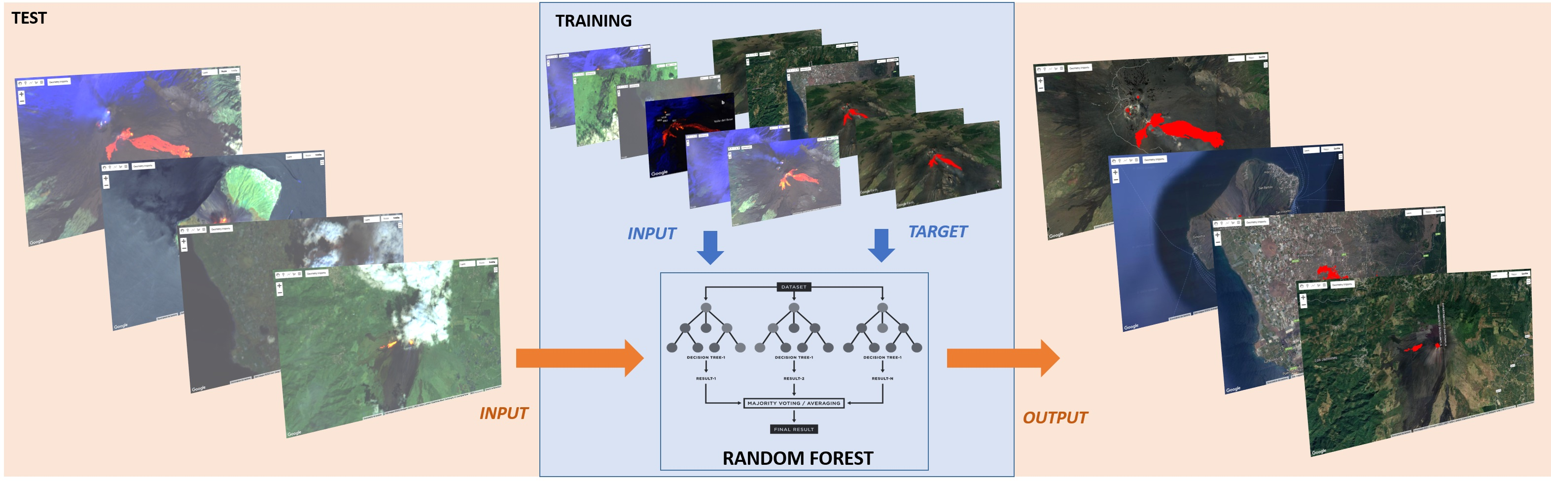
Sentinel-2 consists of a constellation of two identical sun-synchronous satellites, Sentinel-2A (S2A) and Sentinel-2B (S2B), launched in 2015 and 2017, respectively. The revisit frequency of one satellite is 10 days, resulting in a global revisit frequency of 5 days for the constellation. Both satellites are equipped with a MultiSpectral Instrument (MSI) with 13 bands at 10 m spatial resolutions in the visible and near-infrared, at 20 m spatial resolution in the red edge and shortwave infrared part of the spectrum, and at 60 m spatial resolution in the atmospheric bands (“Aerosol,” “Water vapor,” and “Cirrus”). Sentinel-2 (S2) images are made available at different product levels, namely Level-1C (orthorectified TOA) and Level-2A (orthorectified atmospherically corrected surface reflectance SR), in Google Earth Engine [72].
The images used in these studies are Level-1C containing 13 UINT16 spectral bands representing TOA reflectance scaled by 10,000. For this study, TOA reflectance measurements were converted to radiance in [W m−2 sr−1 µm−1].
In particular, radiances measured at bands B2 (496.6 nm (S2A)/492.1 nm (S2B)), B3 (560 nm (S2A)/559 nm (S2B)), B4 (664.5 nm (S2A)/665 nm (S2B)), B5 (703.9 nm (S2A)/703.8 nm (S2B)), B8A (864.8 nm (S2A)/864 nm (S2B)), B11 (1613.7 nm (S2A)/1610.4 nm (S2B)), and B12 (2202.4 nm (S2A)/2185.7 nm (S2B)) are used and referred to as L0.4, L0.5, L0.6, L0.7, L0.8, L1.6, and L2.2, respectively.
The images that have been used for the training and testing phase are reported in Table 2, and the images for the testing phase are also shown in Figure 2.

3. Methods

We aim to design a robust supervised classifier using high spatial resolution images from the S2-MSI exploiting spectral bands ranging from visible to short infrared, which are relevant in the detection of thermal anomalies. This generalized supervised classifier uses spectral information provided by the S2-MSI to learn to discriminate between thermal anomalies (class 1, thermal anomaly) with a high accuracy level, i.e., being able to detect lower intensities changes and background (class 0, background) characterized by different spectral features, e.g., snow and/or clouds. The workflow representing the three main steps of the ML algorithm is illustrated in Figure 3.

3.1. Features Selection

Firstly, discriminative features need to be selected in order to teach the ML model to recognize anomalies. Two sets of bands are considered as the candidate input of the ML model. The first set of features (Feat1) relies on a set of bands that were already being used to recognize, successfully, mid to extreme anomalies worldwide while minimizing false alarms [29]. In particular, three normalized indexes have been used for volcanic applications [28,29], as defined in Equations (1)–(3):
NHI SWNIR = L 1.6 L 0.8 L 1.6 + L 0.8
NHI SWIR = L 2.2 L 1.6 L 2.2 + L 1.6
ND = L 2.2 L 0.8 L 2.2 + L 0.8
where NHISWNIR is a normalized hotspot index (NHI) based on SWIR1 and NIR, NHISWIR is based on SWIR2 and SWIR1, and ND is a normalized index based on SWIR2 and NIR [28,29]. Increased accuracy is achieved by using additional spectral tests based on the bands Red Edge 1, SWIR1, and SWIR2.
The second set of features (Feat2) takes advantage of the fact that the model can discriminate volcanic anomalies and the heterogeneous background, learning the spectral signatures of the monitored surfaces and thermal emissions [73,74,75,76]. In fact, especially when thermal anomalies are less intense, thus affecting less S2-MSI infrared bands, contributions from the other bands may help identify spectral signatures of the erupted bodies and background. In particular, learning spectral signatures of different backgrounds, and having a well-known spectral response, such as clouds, snow, and vegetation, helps reduce false negative detection. Thus, Feat 2 contains radiances from VIS to SWIR. In Table 3, both the feature sets, namely Feat 1 and Feat 2, are summarized.
At this point, training and testing datasets are created for the investigated eruptions using the S2-MSI images listed in Table 2. For each eruptive event, the input and target images need to be prepared. All the bands used in the feature sets (see Table 3) are normalized by using the z-score normalization, accounting for the differences in the range of the selected variables.
The target consists in a binary image where 1 is associated with the thermal anomalies and 0 with the background. Target images have been retrieved using high spatial resolution images from the S2-MSI. The location of true hot pixels building up the actual lava flow map in the S2-MSI image was determined manually by visual inspection [41,77] via expert human analysis for each of the scenes. In particular, in order to do that, experts draw in GEE the target upon the False RGB S2-MSI image (B12-B11-B5) that is able to highlight the incandescent components. Unfortunately, it is not always possible to conclusively define the boundaries of the hot pixels’ clusters, i.e., discriminating where the hot target ends and the background begins [41]. This introduces a degree of subjectivity in any true hot pixel map [78]. However, it is possible to at least assess the algorithm performance with respect to an expert human analyst, i.e., computing accuracy and other performance indexes using the target retrieved by the experts [41]. As a consequence, the target/actual maps have the same spatial resolution as the lowest spatial resolution among the adopted S2-MSI bands, namely a 20 m ground sampling distance. Since lower thermal anomalies are more difficult to be detected, when selecting a target in the training images, we included the pixels with lower temperatures. B12, which is the most suitable band to focus on lower temperatures for the Wien law, has a minimum radiance value of 0.68 [W m−2 sr−1 µm−1] among the anomalous thermal pixels selected as the target.
For both the trained models, the test phase involves images never seen before from the Etna, Stromboli, Cumbre Vieja, and Pacaya volcanoes. As regards the background, pixels belonging to different kinds of backgrounds are provided, namely soil, clouds, snow, rocks, plume, vegetation, and housing. In general, this allows the model to discriminate spectral responses in the selected bands, especially when anomalies are subtle and thus close to the decision boundaries.

3.2. Model Identification

As for the ML algorithm, we used the Random Forest (RF) model for two main reasons. On the one hand, we want to exploit the ability of the decision trees building up the RF to tune their decision rules, i.e., discriminating the spectral features of thermal anomalies from the rest, based on the training data. On the other hand, we adopt an RF rather than a single decision tree to reduce overfitting, to improve generalization since the subset of the training samples is used for each tree, and to enhance the stability since the final outcome is based on several of the decision tree outcomes [79]. The decision tree is a supervised ML model able to make predictions based on simple decision rules inferred from input features during the training phase. The RF is made by a predefined number of decision trees exploiting the bagging technique to make a prediction [80]. In particular, each decision tree is trained independently using samples of the original training dataset with replacement, and their results are combined to get the final RF outcome based on the majority voting [48].
A parameter to set in the RF is the number of trees; here, a number of 100 trees is chosen since it represents a good trade-off between complexity and performance, i.e., a higher number of trees did not improve the performance so to justify the higher complexity. During the training phase, RF learns from data the best decision rules to minimize the error between the target and the model output. In particular, an RF for each set of features is trained, namely RF1 and RF2 being trained with Feat1 and Feat2, respectively (see Table 3).

3.3. Performance Evaluation

Finally, the performance evaluation step is performed using different metrics which have been widely employed to quantify the goodness of the fit between the real and calculated lava flow areas [5] based on the areal dimensions of the calculated (test area) and actual lava flow fields. We avoid the use of indexes accounting for the true negative (TN), pixels correctly classified as background pixels, such as the false positive rate (FPR), because for imbalanced datasets, such as in this case (more background-negative than anomalous-positive pixels), this model’s performance index would be largely biased by the TN. A larger number of negative samples, such as in this case, would lead to a high TN and, thus, low FPR. However, this would not reflect the model’s capability to correctly identify a thermal anomaly but the background instead. Since we are focused on the positive class, i.e., identifying thermal anomalies, we consider the following indexes more appropriate for our task [81]:
  • accuracy (ACC) = A ( t e s t     r e a l ) A ( t e s t     r e a l )
  • precision (also known as the positive predictive value, PPV) = A ( t e s t     r e a l ) A ( t e s t   )
  • recall (also known as the true positive rate, TPR) = A ( t e s t     r e a l ) A ( r e a l   )
ACC involves A(test ∩ real) and A(test ∪ real), which are the areas of the intersection and union between the calculated and actual lava flows (the targets), respectively. This index evaluates the difference in the emplacement between the diverse lava flow fields and the goodness of the maps obtained. PPV indicates the percentage of calculated lava flow fields covered by the actual lava flows. TPR is similar to the previous one and evaluates the percentage of the actual lava flow field covered by the calculated lava flows. The three indices have values between 0 and 1, with 1 for a complete overlap, i.e., the calculated area coincides totally with the actual lava flow field, and 0 for a maximum error, i.e., lack of common areas between the calculated and actual lava flows. The comparison between the ACC, PPV, and TPR gives insights into how the calculated emplacements change with respect to the actual areas. Precisely, the testing area underestimates the actual one if the PPV is higher than the ACC, while it overestimates if the TPR is greater than the ACC [82,83,84,85].
The fixed threshold algorithm is implemented for comparison purposes, considering the well-known decision rules [28].

4. Results

We trained the RF models with multiple volcanic eruptive events using training and testing images as the set of the S2-MSI acquisitions reported in Table 2. During the training phase, we used, as a target for each volcano case study, portions of the lava flows manually selected and labelled as the anomaly and background.
For each variable in the feature space, an importance value is retrieved from the random forest models [86,87], showing how much relevant and discriminative the variable is in the random forest model for the classification task under investigation. These values are computed as follows: Since the features for the internal nodes are selected with Gini impurity or information gain, how each feature decreases the impurity of the split (the feature with the highest decrease is selected for the internal node) can be measured. For each feature, we can collect how, on average, it decreases the impurity. The average over all the trees in the forest is the measure of the feature importance.
The importance values’ percentages for both RF1 and RF2 are shown in Figure 4. Figure 5 and Figure 6 show the test set, in particular, the S2-MSI False RGB (B12-B8A-B5) images, the RF outcomes, and the fixed threshold outcomes for Etna on 21 February 2021 (Figure 5a–d), Stromboli on 27 July 2019 (Figure 5e–h), Cumbre Vieja on 25 September 2021 (Figure 6a–d), and Pacaya on 31 October 2020 (Figure 6e–h). The S2-MSI False RGB (B12-B8A-B5) images with an appropriate stretch are shown to highlight less intense anomalies otherwise not clearly visible.

5. Discussion

Our results highlight the ability of the Random Forest to learn the detection of low to extreme thermal anomalies using spectral observations. In particular, both the proposed RF models show a good generalization capability, being able to map thermal anomalies over several different volcanoes. We obtained a good performance level and an accuracy that is around 0.9 for both RF1 and RF2 as the average for all the volcanoes’ study cases with respect to 0.83 for the fixed threshold (FT) algorithm (Table 4). In particular, they perform well even when applied to volcanoes never seen during the training phase, i.e., Pacaya. In fact, training the random forest with wide-spanning eruptive events in different areas in the world allows us to learn the best features to correctly classify cooler to incandescent thermal anomalies with a low number of missed detections, as shown by the TPR index (Table 4). The first improvement is achieved by RF1 with respect to the FT algorithm. Using the NIR and SWIR bands (that are usually adopted to monitor mid to high thermal features), RF1 is able to detect subtler anomalies. This is due to the fact that RF1 has tuned its parameters from the data, thus being able to generalize better in order to account for subtle changes. An example of this is shown in Figure 6b,c, where the FT is only able to detect the hotter portion of the volcanic anomaly in Cumbre Vieja while RF1 is able to map far more anomalies. A further improvement is achieved with RF2, which, by using visible bands, learns the spectral signatures of the trained, monitored surfaces. In fact, when the emitted radiance is low, the reflected radiance becomes dominant, and thus, the capability of the model to learn them allows us to reduce the number of false negatives. This is reflected in a higher TPR.
From Table 4, we can compare the performance of the three algorithms, and we can state that RFs outperform the FT. Furthermore, even though RF2 has slightly higher TPR and ACC for the reasons previously stated, the performances of RF1 and RF2 are very similar. On the one hand, ACC and TPR are higher using RFs than the fixed threshold algorithm, meaning that RFs are able to well predict thermal anomalies with a lower number of false negative detections with respect to the fixed threshold approach. In other words, RFs underestimate less than the fixed threshold algorithms. This is due to the fact that the RF is trained to detect even lower thermal anomalies, as can be noticed in all the study cases presented. On the other hand, PPV is high for RFs but lower than the fixed threshold approach, meaning that RFs have a higher number of false positives, and thus, RFs overestimate more with respect to fixed threshold algorithms. This is expected because, being that the RFs are able to detect, also, low thermal anomalies, false positives due to hot reflections may be detected in areas very close to volcanic anomalies, as in the case of Cumbre Vieja, where false positives are clearly visible due to the presence of thermal reflection in clouds. Thus, the higher value of PPV for the fixed threshold approach is due to the fact that the thresholds used are more conservative in preventing false positive detections. However, this leads the fixed threshold algorithm to miss anomalies, as it is shown in Figure 5 and Figure 6.
This means that even though some of the anomalies detected by the RFs are due to reflection (a lower PPV), some missed by the FT are instead detected by the RFs, being subtle anomalies (a higher TPR). In particular, a bigger portion of real anomalies is detected than the ones misclassified as false anomalies, resulting in a greater accuracy estimated using RFs than the FT, i.e., 0.9 to 0.91 and 0.83, respectively (Figure 7).
In summary, RFs achieve a better compromise than fixed threshold algorithms in terms of missed detection and false alarms. In fact, since all the performance indexes are high and belong to a narrow range of around 0.9, i.e., (0.87, 0.92) and (0.89, 0.91) for RF1 and RF2, respectively, there is not a clear underestimation/overestimation tendency of the RF models. On the contrary, the fixed threshold algorithm has lower performance indexes belonging to a wider range, i.e.,(0.79, 0.99), showing a clear underestimation tendency of this model, i.e., its precision is far higher than its accuracy (see Figure 7).
In particular, we considered the Stromboli test case, i.e., the 27 July 2019 eruption, which was characterized by a lava overflow from the summit crater. This is shown in the S2-MSI False RGB with a stretch that helps highlight the lower thermal anomalies. Furthermore, four fires that developed on the South-East side of the island are clearly visible, as well (Figure 5e). The emplacements of the overflows have been verified from the thermal camera of the INGV network [www.ct.ingv.it (accessed on 15 July 2022)]. The algorithm based on the fixed thresholds, of which it has been shown to work well globally, misses the cooler anomalies, namely the thinner overflow and the one out of the four bigger fires (Figure 5f). The thermal anomaly map of the RF1 model is able to detect some pixels of the cooler overflow, the incandescent overflow, and the four fires (Figure 5g). A further improvement is shown using RF2, where more pixels belonging to the thinner overflow are detected (Figure 5h). In order to assess the advantages of using a data-driven approach with respect to a fixed threshold algorithm, we applied RF algorithms to another test case image from Etna, 11 February 2022, where the cooling portions of lava flows are visible. The first available S2-MSI image was acquired on 11 February 2022, where the cooling portions of the lava flows are visible. As can be noticed in Figure 8, a greater portion of thermal anomalies is detected by the RFs (Figure 8c,d) than by the fixed threshold algorithm (Figure 8b). In particular, lower thermal anomalies are detected, as is confirmed by the false RGB in Figure 8. These results show the effectiveness of the RF data-driven approach in detecting low to extreme thermal anomalies. Although six scenes for training have been used, being a pixel-based approach, the number of samples considered is hundreds of thousands, accounting for different thermal features and enough to train machine learning techniques. Nevertheless, future works will focus on increasing the dataset size to make the model more and more generalizable.

6. Conclusions

We have presented a robust data-driven strategy based on the random forest model to map lower to extreme thermal anomalies using Sentinel-2 high spatial resolution images. We have exploited the decision rules strategy of decision trees and the generalization capability of RF models to tune relevant spectral features to train satellite data acquired over different volcanoes. This allowed us to automatically map thermal anomalies avoiding fixed a priori thresholds. We have used two sets of input features, obtaining two RF models that have shown similar performances. It is worth noting that also using visible bands allows us to enhance the model’s capability to detect less intense anomalies by exploiting the learned spectral signatures of the monitored surfaces.
RFs trained on multiple volcanoes and eruptions are able to well-classify, from less to very intense, volcanic anomalies and also volcanoes never seen before, i.e., Pacaya, showing great generalization capabilities. This implies that the proposed data-driven approach shows the potential to be used over different volcanoes, obtaining a model available and ready to be used once an eruption occurs worldwide. However, further expansion of the training datasets to more study cases and volcanoes in the future is needed to better generalize this model for lava flow mapping worldwide. Thus, the next steps involve increasing the dataset sizes and, thus, making a GEE app available to be used on a global scale.

Author Contributions

Conceptualization, C.C.; methodology, C.C. and E.A.; software, C.C., E.A. and F.T.; validation, F.T. and C.D; formal analysis, C.D.N.; investigation, C.C.; resources, E.A.; data curation, E.A. and C.C.; writing—original draft preparation, C.C.; writing—review and editing, F.T.; visualization, C.D.N.; supervision, C.D.N.; project administration, C.D.N. All authors have read and agreed to the published version of the manuscript.

Funding

This research was funded by [ATHOS Research Programme] (OB.FU. 0867.010).

Data Availability Statement

Data used in this paper are available in GEE.

Acknowledgments

This work was developed within the framework of the Laboratory of Technologies for Volcanology (TechnoLab) at the INGV in Catania (Italy). We gratefully acknowledge the funding support from the ATHOS (Advanced Tools and metHods for cOmputational fluid dynamicS) Research Programme.

Conflicts of Interest

The authors declare no conflict of interest.

References

  1. Harris, A. Thermal Remote Sensing of Active Volcanoes: A User’s Manual; Cambridge University Press: Cambridge, UK, 2013. [Google Scholar]
  2. Ganci, G.; Cappello, A.; Bilotta, G.; Del Negro, C. How the variety of satellite remote sensing data over volcanoes can assist hazard monitoring efforts: The 2011 eruption of Nabro volcano. Remote Sens. Environ. 2020, 236, 111426. [Google Scholar] [CrossRef]
  3. Ganci, G.; Bilotta, G.; Cappello, A.; Herault, A.; Del Negro, C. HOTSAT: A multiplatform system for the thermal monitoring of volcanic activity using satellite data. Geol. Soc. Lond. Spec. Publ. 2016, 426, 207–221. [Google Scholar] [CrossRef]
  4. Abrams, M.; Abbott, E.; Kahle, A. Combined use of visible, reflected infrared, and thermal infrared images for mapping Hawaiian lava flows. J. Geophys. Res. 1991, 96, 475–484. [Google Scholar] [CrossRef]
  5. Corradino, C.; Ganci, G.; Bilotta, G.; Cappello, A.; Del Negro, C.; Fortuna, L. Smart decision support systems for volcanic applications. Energies 2019, 12, 1216. [Google Scholar] [CrossRef]
  6. Patrick, M.R.; Kauahikaua, J.; Orr, T.; Davies, A.; Ramsey, M. Operational thermal remote sensing and lava flow monitoring at the Hawaiian Volcano Observatory. Geol. Soc. Lond. Spec. Publ. 2016, 426, 489–503. [Google Scholar] [CrossRef]
  7. Cappello, A.; Ganci, G.; Bilotta, G.; Herault, A.; Zago, V.; Del Negro, C. Satellite-driven modeling approach for monitoring lava flow hazards during the 2017 Etna eruption. Ann. Geophys. 2018, 61, 13. [Google Scholar] [CrossRef]
  8. Pergola, N.; D’Angelo, G.; Lisi, M.; Marchese, F.; Mazzeo, G.; Tramutoli, V. Time domain analysis of robust satellite techniques (RST) for near real-time monitoring of active volcanoes and thermal precursor identification. Phys. Chem. Earth Parts A/B/C 2009, 34, 380–385. [Google Scholar] [CrossRef]
  9. Coppola, D.; Laiolo, M.; Cigolini, C.; Delle Donne, D.; Ripepe, M. Enhanced volcanic hot-spot detection using MODIS IR data: Results from the MIROVA system. Geol. Soc. Lond. Spec. Publ. 2016, 426, 181–205. [Google Scholar] [CrossRef]
  10. Vicari, A.; Bilotta, G.; Bonfiglio, S.; Cappello, A.; Ganci, G.; Hèrault, A.; Rustico, E.; Gallo, G.; Del Negro, C. LAV@ HAZARD: A web-GIS interface for volcanic hazard assessment. Ann. Geophys. 2011, 54. [Google Scholar] [CrossRef]
  11. Ganci, G.; Harris, A.J.; Del Negro, C.; Guéhenneux, Y.; Cappello, A.; Labazuy, P.; Calvari, S.; Gouhier, M. A year of lava fountaining at Etna: Volumes from SEVIRI. Geophys. Res. Lett. 2012, 39. [Google Scholar] [CrossRef]
  12. Ganci, G.; Vicari, A.; Cappello, A.; Del Negro, C. An emergent strategy for volcano hazard assessment: From thermal satellite monitoring to lava flow modeling. Remote Sens. Environ. 2012, 119, 197–207. [Google Scholar] [CrossRef]
  13. Del Negro, C.; Cappello, A.; Ganci, G. Quantifying lava flow hazards in response to effusive eruption. Geol. Soc. Am. Bull. 2016, 28, 752–763. [Google Scholar] [CrossRef]
  14. Blackett, M. Review of the utility of infrared remote sensing for detecting and monitoring volcanic activity with the case study of shortwave infrared data for Lascar Volcano from 2001–2005. Geol. Soc. Lond. Spec. Publ. 2013, 380, 107–135. [Google Scholar] [CrossRef]
  15. Kubanek, J.; Richardson, J.A.; Charbonnier, S.J.; Connor, L.J. Lava flow mapping and volume calculations for the 2012–2013 Tolbachik, Kamchatka, fissure eruption using bistatic TanDEM-X InSAR. Bull. Volcanol. 2015, 77, 106. [Google Scholar] [CrossRef]
  16. Bonaccorso, A.; Caltabiano, T.; Currenti, G.; Del Negro, C.; Gambino, S.; Ganci, G.; Giammanco, S.; Greco, F.; Pistorio, A.; Salerno, G.; et al. Dynamics of a lava fountain revealed by geophysical, geochemical and thermal satellite measurements: The case of the 10 April 2011 Mt. Etna eruption. Geophys. Res. Lett. 2011, 38, L24307. [Google Scholar]
  17. Wooster, M.J.; Roberts, G.; Perry, G.L.W.; Kaufman, Y.J. Retrieval of biomass combustion rates and totals from fire radiative power observations: FRP derivation and calibration relationships between biomass consumption and fire radiative energy release. J. Geophys. Res. Atmos. 2005, 110, 311. [Google Scholar] [CrossRef]
  18. Wooster, M.J.; Zhukov, B.; Oertel, D. Fire radiative energy for quantitative study of biomass burning: Derivation from the BIRD experimental satellite and comparison to MODIS fire products. Remote Sens. Environ. 2003, 86, 83–107. [Google Scholar] [CrossRef]
  19. Zakšek, K.; Hort, M.; Lorenz, E. Satellite and ground based thermal observation of the 2014 effusive eruption at Stromboli volcano. Remote Sens. 2015, 7, 17190–17211. [Google Scholar] [CrossRef]
  20. Vulpiani, G.; Ripepe, M.; Valade, S. Mass discharge rate retrieval combining weather radar and thermal camera observations. J. Geophys. Res. Solid Earth 2016, 121, 5679–5695. [Google Scholar] [CrossRef]
  21. Bato, M.G.; Froger, J.L.; Harris, A.J.L.; Villeneuve, N. Monitoring an effusive eruption at Piton de la Fournaise using radar and thermal infrared remote sensing data: Insights into the October 2010 eruption and its lava flows. Geol. Soc. Lond. Spec. Publ. 2016, 426, 533–552. [Google Scholar] [CrossRef]
  22. Bisson, M.; Spinetti, C.; Andronico, D.; Palaseanu-Lovejoy, M.; Buongiorno, M.F.; Alexandrov, O.; Cecere, T. Ten years of volcanic activity at Mt Etna: High-resolution mapping and accurate quantification of the morphological changes by Pleiades and Lidar data. Int. J. Appl. Earth Obs. Geoinf. 2021, 102, 102369. [Google Scholar] [CrossRef]
  23. Bonaccorso, A.; Currenti, G.; Linde, A.; Sacks, S. New data from borehole strainmeters to infer lava fountain sources (Etna 2011–2012). Geophys. Res. Lett. 2013, 40, 3579–3584. [Google Scholar] [CrossRef]
  24. Ganci, G.; Cappello, A.; Bilotta, G.; Herault, A.; Zago, V.; Del Negro, C. Mapping volcanic deposits of the 2011–2015 Etna eruptive events using satellite remote sensing. Front. Earth Sci. 2018, 6, 83. [Google Scholar] [CrossRef]
  25. Slatcher, N.; James, M.; Calvari, S.; Ganci, G.; Browning, J. Quantifying effusion rates at active volcanoes through integrated time-lapse laser scanning and photography. Remote Sens. 2015, 7, 14967–14987. [Google Scholar] [CrossRef]
  26. Blackett, M. An overview of infrared remote sensing of volcanic activity. J. Imaging 2017, 3, 13. [Google Scholar] [CrossRef]
  27. Pieper, M.; Manolakis, D.; Truslow, E.; Weisner, A.; Bostick, R.; Cooley, T. Wavelength Calibration Correction Technique for Improved Emissivity Retrieval. IEEE J. Sel. Top. Appl. Earth Obs. Remote Sens. 2020, 13, 642–648. [Google Scholar] [CrossRef]
  28. Marchese, F.; Genzano, N.; Neri, M.; Falconieri, A.; Mazzeo, G.; Pergola, N. A multi-channel algorithm for mapping volcanic thermal anomalies by means of Sentinel-2 MSI and Landsat-8 OLI data. Remote Sens. 2019, 11, 2876. [Google Scholar] [CrossRef]
  29. Genzano, N.; Pergola, N.; Marchese, F. A Google Earth Engine tool to investigate, map and monitor volcanic thermal anomalies at global scale by means of mid-high spatial resolution satellite data. Remote Sens. 2020, 12, 3232. [Google Scholar] [CrossRef]
  30. Corradino, C.; Bilotta, G.; Cappello, A.; Fortuna, L.; Del Negro, C. Combining Radar and Optical Satellite Imagery with Machine Learning to Map Lava Flows at Mount Etna and Fogo Island. Energies 2021, 14, 197. [Google Scholar] [CrossRef]
  31. Plank, S.; Marchese, F.; Genzano, N.; Nolde, M.; Martinis, S. The short life of the volcanic island New Late’iki (Tonga) analyzed by multi-sensor remote sensing data. Sci. Rep. 2020, 10, 1–15. [Google Scholar] [CrossRef]
  32. Marchese, F.; Filizzola, C.; Lacava, T.; Falconieri, A.; Faruolo, M.; Genzano, N.; Mazzeo, G.; Pietrapertosa, C.; Pergola, N.; Tramutoli, V.; et al. Correction: Marchese et al. Mt. Etna Paroxysms of February–April 2021 Monitored and Quantified through a Multi-Platform Satellite Observing System. Remote Sens. 2021, 13, 3074. Remote Sens. 2022, 14, 2746. [Google Scholar] [CrossRef]
  33. Tramutoli, V.; Filizzola, C.; Genzano, N.; Lisi, M. Robust satellite techniques for detecting preseismic thermal anomalies. In Pre-Earthquake Processes: A Multidisciplinary Approach to Earthquake Prediction Studies; American Geophysical Union: Washington, DC, USA, 2018; pp. 243–258. [Google Scholar]
  34. Steffke, A.M.; Harris, A.J. A review of algorithms for detecting volcanic hot spots in satellite infrared data. Bull. Volcanol. 2011, 73, 1109–1137. [Google Scholar] [CrossRef]
  35. Jiao, Z.H.; Zhao, J.; Shan, X. Pre-seismic anomalies from optical satellite observations: A review. Nat. Hazards Earth Syst. Sci. 2018, 18, 1013–1036. [Google Scholar] [CrossRef]
  36. Wright, R.; Flynn, L.P.; Garbeil, H.; Harris, A.J.; Pilger, E. MODVOLC: Near-real-time thermal monitoring of global volcanism. J. Volcanol. Geotherm. Res. 2004, 135, 29–49. [Google Scholar] [CrossRef]
  37. Higgins, J.; Harris, A. VAST: A program to locate and analyse volcanic thermal anomalies automatically from remotely sensed data. Comput. Geosci. 1997, 23, 627–645. [Google Scholar] [CrossRef]
  38. Giglio, L.; Schroeder, W.; Justice, C.O. The collection 6 MODIS active fire detection algorithm and fire products. Remote Sens. Environ. 2016, 178, 31–41. [Google Scholar] [CrossRef]
  39. Murphy, S.W.; Oppenheimer, C.; De Souza Filho, C.R. Calculating radiant flux from thermally mixed pixels using a spectral library. Remote Sens. Environ. 2014, 142, 83–94. [Google Scholar] [CrossRef]
  40. Hua, L.; Shao, G. The progress of operational forest fire monitoring with infrared remote sensing. J. For. Res. 2017, 28, 215–229. [Google Scholar] [CrossRef]
  41. Murphy, S.W.; de Souza Filho, C.R.; Wright, R.; Sabatino, G.; Pabon, R.C. HOTMAP: Global hot target detection at moderate spatial resolution. Remote Sens. Environ. 2016, 177, 78–88. [Google Scholar] [CrossRef]
  42. Layana, S.; Aguilera, F.; Rojo, G.; Vergara, Á.; Salazar, P.; Quispe, J.; Urra, P.; Urrutia, D. Volcanic Anomalies monitoring System (VOLCANOMS), a low-cost volcanic monitoring system based on Landsat images. Remote Sens. 2020, 12, 1589. [Google Scholar] [CrossRef]
  43. Massimetti, F.; Coppola, D.; Laiolo, M.; Valade, S.; Cigolini, C.; Ripepe, M. Volcanic hot-spot detection using SENTINEL-2: A comparison with MODIS–MIROVA thermal data series. Remote Sens. 2020, 12, 820. [Google Scholar] [CrossRef] [Green Version]
  44. Corradino, C.; Amato, E.; Torrisi, F.; Del Negro, C. Towards an automatic generalized machine learning approach to map lava flows. In Proceedings of the 2021 17th International Workshop on Cellular Nanoscale Networks and their Applications (CNNA), Catania, Italy, 29 September–1 October 2021; pp. 1–4. [Google Scholar] [CrossRef]
  45. Amato, E.; Corradino, C.; Torrisi, F.; Del Negro, C. Mapping lava flows at Etna Volcano using Google Earth Engine, open-access satellite data, and machine learning. In Proceedings of the 2021 International Conference on Electrical, Computer, Communications and Mechatronics Engineering (ICECCME), Mauritius, 7–8 October 2021; pp. 1–6. [Google Scholar] [CrossRef]
  46. Anantrasirichai, N.; Biggs, J.; Albino, F.; Hill, P.; Bull, D. Application of Machine Learning to Classification of Volcanic Deformation in Routinely Generated InSAR Data. J. Geophys. Res. Solid Earth 2018, 123, 6592–6606. [Google Scholar] [CrossRef]
  47. Lary, D.J.; Alavi, A.H.; Gandomi, A.H.; Walker, A.L. Machine learning in geosciences and remote sensing. Geosci. Front. 2016, 7, 3–10. [Google Scholar] [CrossRef]
  48. Li, C.; Wang, J.; Wang, L.; Hu, L.; Gong, P. Comparison of classification algorithms and training sample sizes in urban land classification with Landsat thematic mapper imagery. Remote Sens. 2014, 6, 964–983. [Google Scholar] [CrossRef]
  49. Lüdtke, A.; Jerosch, K.; Herzog, O.; Schlüter, M. Development of a machine learning technique for automatic analysis of seafloor image data: Case example, Pogonophora coverage at mud volcanoes. Comput. Geosci. 2012, 39, 120–128. [Google Scholar] [CrossRef]
  50. Corradino, C.; Ganci, G.; Cappello, A.; Bilotta, G.; Calvari, S.; Del Negro, C. Recognizing Eruptions of Mount Etna through Machine Learning using Multiperspective Infrared Images. Remote Sens. 2020, 12, 970. [Google Scholar] [CrossRef]
  51. Zhang, M.; Zhang, M.; Yang, H.; Jin, Y.; Zhang, X.; Liu, H. Mapping regional soil organic matter based on sentinel-2a and modis imagery using machine learning algorithms and google earth engine. Remote Sens. 2021, 13, 2934. [Google Scholar] [CrossRef]
  52. James, G.; Witten, D.; Hastie, T.; Tibshirani, R. An Introduction to Statistical Learning; Springer: New York, NY, USA, 2013; Volume 112, p. 18. [Google Scholar]
  53. Bonaccorso, G. Machine Learning Algorithms; Packt Publishing Ltd.: Birmingham, UK, 2017. [Google Scholar]
  54. Belgiu, M.; Drăguţ, L. Random forest in remote sensing: A review of applications and future directions. ISPRS J. Photogramm. Remote Sens. 2016, 114, 24–31. [Google Scholar] [CrossRef]
  55. Schonlau, M.; Zou, R.Y. The random forest algorithm for statistical learning. Stata J. 2020, 20, 3–29. [Google Scholar] [CrossRef]
  56. Paul, A.; Mukherjee, D.P.; Das, P.; Gangopadhyay, A.; Chintha, A.R.; Kundu, S. Improved random forest for classification. IEEE Trans. Image Processing 2018, 27, 4012–4024. [Google Scholar] [CrossRef]
  57. Longpré, M.A. Reactivation of Cumbre Vieja volcano. Science 2021, 374, 1197–1198. [Google Scholar] [CrossRef] [PubMed]
  58. Carracedo, J.C.; Troll, V.R.; Day, J.M.; Geiger, H.; Aulinas, M.; Soler, V.; Deegan, F.M.; Perez-Torrado, F.J.; Gisbert, G.; Gazel, E.; et al. The 2021 eruption of the Cumbre Vieja Volcanic Ridge on La Palma, Canary Islands. Geol. Today 2022, 38, 94–107. [Google Scholar] [CrossRef]
  59. Eibl, E.P.; Thordarson, T.; Höskuldsson, Á.; Gudnason, E.Á.; Dietrich, T.; Hersir, G.P.; Ágústsdóttir, T. Evolving Shallow-conduit Container Affects the Lava Fountaining during the 2021 Fagradalsfjall Eruption, Iceland. Res. Sq. 2022. [Google Scholar] [CrossRef]
  60. Pedersen, G.B.; Belart, J.M.; Óskarsson, B.V.; Gudmundsson, M.T.; Gies, N.; Högnadóttir, T.; Hjartardóttir, Á.R.; Pinel, V.; Berthier, E.; Dürig, T.; et al. Volume, effusion rate, and lava transport during the 2021 Fagradalsfjall eruption: Results from near real-time photogrammetric monitoring. Geophys. Res. Lett. 2022, 49, e2021GL097125. [Google Scholar] [CrossRef]
  61. Calvari, S.; Di Traglia, F.; Ganci, G.; Giudicepietro, F.; Macedonio, G.; Cappello, A.; Nolesini, T.; Pecora, E.; Bilotta, G.; Centorrino, V.; et al. Overflows and pyroclastic density currents in March-April 2020 at Stromboli volcano detected by remote sensing and seismic monitoring data. Remote Sens. 2020, 12, 3010. [Google Scholar] [CrossRef]
  62. Corradino, C.; Amato, E.; Torrisi, F.; Calvari, S.; Del Negro, C. Classifying Major Explosions and Paroxysms at Stromboli Volcano (Italy) from Space. Remote Sens. 2021, 13, 4080. [Google Scholar] [CrossRef]
  63. Aiuppa, A.; Bertagnini, A.; Métrich, N.; Moretti, R.; Di Muro, A.; Liuzzo, M.; Tamburello, G. A model of degassing for Stromboli volcano. Earth Planet. Sci. Lett. 2010, 295, 195–204. [Google Scholar] [CrossRef]
  64. Rose, W.I.; Palma, J.L.; Wolf, R.E.; Gomez, R.M. A 50 yr eruption of a basaltic composite cone: Pacaya, Guatemala. Geol. Soc. Am. Spec. Pap. 2013, 498, 1–21. [Google Scholar]
  65. Schaefer, L.N.; Lu, Z.; Oommen, T. Post-eruption deformation processes measured using ALOS-1 and UAVSAR InSAR at Pacaya Volcano, Guatemala. Remote Sens. 2016, 8, 73. [Google Scholar]
  66. Ganci, G.; Cappello, A.; Zago, V.; Bilotta, G.; Herault, A.; Del Negro, C. 3D Lava flow mapping of the 17–25 May 2016 Etna eruption using tri-stereo optical satellite data. Ann. Geophys. 2018, 62. [Google Scholar] [CrossRef]
  67. Bonaccorso, A.; Calvari, S.; Currenti, G.; Del Negro, C.; Ganci, G.; Linde, A.; Napoli, R.; Sacks, S.; Sicali, A. From source to surface: Dynamics of Etna’s lava fountains investigated by continuous strain, magnetic, ground and satellite thermal data. Bull. Volcanol. 2013, 75, 690. [Google Scholar] [CrossRef]
  68. Marchese, F.; Filizzola, C.; Lacava, T.; Falconieri, A.; Faruolo, M.; Genzano, N.; Mazzeo, G.; Pietrapertosa, C.; Pergola, N.; Tramutoli, V.; et al. Etna paroxysms of February–April 2021 monitored and quantified through a multi-platform satellite observing system. Remote Sens. 2021, 13, 3074. [Google Scholar] [CrossRef]
  69. Calvari, S.; Bonaccorso, A.; Ganci, G. Anatomy of a Paroxysmal Lava Fountain at Etna Volcano: The Case of the 12 March 2021, Episode. Remote Sens. 2021, 13, 3052. [Google Scholar] [CrossRef]
  70. Torrisi, F.; Folzani, F.; Corradino, C.; Amato, E.; Del Negro, C. Detecting Volcanic Ash Plume Components from Space using Machine Learning Techniques. Earth Space Sci. Open Arch. 2021, 1. [Google Scholar] [CrossRef]
  71. Torrisi, F. Automatic approach to detect volcanic plumes using SEVIRI data and machine learning techniques. Il Nuovo Cim. 45 C 2022, 81. [Google Scholar] [CrossRef]
  72. Gorelick, N.; Hancher, M.; Dixon, M.; Ilyushchenko, S.; Thau, D.; Moore, R. Google Earth Engine: Planetary-scale geospatial analysis for everyone. Remote Sens. Environ. 2017, 202, 18–27. [Google Scholar] [CrossRef]
  73. Spinetti, C.; Mazzarini, F.; Casacchia, R.; Colini, L.; Neri, M.; Behncke, B.; Salvatori, R.; Buongiorno, M.F.; Pareschi, M.T. Spectral properties of volcanic materials from hyperspectral field and satellite data compared with LiDAR data at Mt. Etna. Int. J. Appl. Earth Obs. Geoinf. 2009, 11, 142–155. [Google Scholar] [CrossRef]
  74. Head, E.; Maclean, A.L.; Carn, S. Mapping lava flows from Nyamuragira volcano (1967–2011) with satellite data and automated classification methods. Geomat. Nat. Hazards Risk 2013, 4, 119–144. [Google Scholar] [CrossRef]
  75. Corradino, C.; Ganci, G.; Cappello, A.; Bilotta, G.; Hérault, A.; Del Negro, C. Mapping Recent Lava Flows at Mount Etna Using Multispectral Sentinel-2 Images and Machine Learning Techniques. Remote Sens. 2019, 11, 1916. [Google Scholar] [CrossRef]
  76. Li, L.; Solana, C.; Canters, F.; Kervyn, M. Testing random forest classification for identifying lava flows and mapping age groups on a single Landsat 8 image. J. Volcanol. Geotherm. Res. 2017, 345, 109–124. [Google Scholar] [CrossRef]
  77. Lu, Z.; Rykhus, R.; Masterlark, T.; Dean, K.G. Mapping recent lava flows at Westdahl Volcano, Alaska, using radar and optical satellite imagery. Remote Sens. Environ. 2004, 91, 345–353. [Google Scholar] [CrossRef]
  78. Giglio, L.; Csiszar, I.; Restás, Á.; Morisette, J.T.; Schroeder, W.; Morton, D.; Justice, C.O. Active fire detection and characterization with the advanced spaceborne thermal emission and reflection radiometer (ASTER). Remote Sens. Environ. 2008, 112, 3055–3063. [Google Scholar] [CrossRef]
  79. Hastie, T.; Tibshirani, R.; Friedman, J. Random forests. In The Elements of Statistical Learning; Springer: New York, NY, USA, 2009; pp. 587–604. [Google Scholar]
  80. Ghimire, B.; Rogan, J.; Galiano, V.R.; Panday, P.; Neeti, N. An evaluation of bagging, boosting, and random forests for land-cover classification in Cape Cod, Massachusetts, USA. GIScience Remote Sens. 2012, 49, 623–643. [Google Scholar] [CrossRef]
  81. Bilotta, G.; Cappello, A.; Hérault, A.; Del Negro, C. Influence of topographic data uncertainties and model resolution on the numerical simulation of lava flows. Environ. Model. Softw. 2019, 112, 1–15. [Google Scholar] [CrossRef]
  82. Cappello, A.; Ganci, G.; Calvari, S.; Pérez, N.M.; Hernández, P.A.; Silva, S.V.; Cabral, J.; Del Negro, C.; Vitória, S. Lava flow hazard modeling during the 2014-2015 Fogo eruption, Cape Verde. J. Geophys. Res. Solid Earth 2016, 121, 2290–2303. [Google Scholar] [CrossRef]
  83. Kereszturi, G.; Cappello, A.; Ganci, G.; Procter, J.; Nemeth, K.; Del Negro, C.; Cronin, S.J. Numerical simulation of basaltic lava flows in the Auckland Volcanic Field, New Zealand—Implication for volcanic hazard assessment. Bull. Volcanol. 2014, 76, 879. [Google Scholar] [CrossRef]
  84. Kereszturi, G.; Nemeth, K.; Moufti, M.R.; Cappello, A.; Murcia, H.; Ganci, G.; Del Negro, C.; Procter, J.; Zahran, H.M.A. Emplacement conditions of the 1256 AD Al-Madinah lava flow field in Harrat Rahat, Kingdom of Saudi Arabia—Insights from surface morphology and lava flow simulations. J. Volcanol. Geotherm. Res. 2016, 309, 14–30. [Google Scholar] [CrossRef]
  85. Archer, K.J.; Kimes, R.V. Empirical characterization of random forest variable importance measures. Comput. Stat. Data Anal. 2008, 52, 2249–2260. [Google Scholar] [CrossRef]
  86. Menze, B.H.; Kelm, B.M.; Masuch, R.; Himmelreich, U.; Bachert, P.; Petrich, W.; Hamprecht, F.A. A comparison of random forest and its Gini importance with standard chemometric methods for the feature selection and classification of spectral data. BMC Bioinform. 2009, 10, 213. [Google Scholar] [CrossRef] [Green Version]
  87. Rogers, J.; Gunn, S. Identifying feature relevance using a random forest. In International Statistical and Optimization Perspectives Workshop. In Subspace, Latent Structure and Feature Selection; Springer: Berlin/Heidelberg, Germany, 2005; pp. 173–184. [Google Scholar]
Figure 1. Volcanoes used in the train and test phase for the two models, (a) targeted volcanoes localization, (b) Mt. Etna, (c) Cumbre Vieja, (d) Geldingadalir, (e) Stromboli, and (f) Pacaya. All the images were captured via Google Earth Engine.
Remotesensing 14 04370 g001
Figure 2. Sentinel-2 MSI TOA reflectance images used as the test set for the two models. False RGB (B12, B11, and B5) S2-MSI acquisition over (a) Mt. Etna—21 February 2021—(b) Stromboli—27 July 2019—(c) Cumbre Vieja—25 September 2021—and (d) Pacaya—31 October 2020.
Remotesensing 14 04370 g002
Figure 3. General workflow representing the three main steps of the ML algorithm: features selection, model identification, and performance evaluation.
Remotesensing 14 04370 g003
Figure 4. Feature importance related to the models RF1 (a) and RF2 (b).
Remotesensing 14 04370 g004
Figure 5. Test set: S2-MSI False RGB (B12-B8A-B5) image, the fixed threshold, the RF (NIR and SWIR) and the RF (VIS, NIR, and SWIR) outcomes for Etna on the 21 February 2021, (ad) and Stromboli on the 27 July 2019 (eh). All the images were captured via Google Earth Engine.
Remotesensing 14 04370 g005
Figure 6. Test set: S2-MSI False RGB (B12-B8A-B5) image, the fixed threshold, the RF (NIR and SWIR) and the RF (VIS, NIR, and SWIR) outcomes for Cumbre Vieja on the 25 September 2021 (ad) and Pacaya on the 31 October 2020 (eh). All the images were captured via Google Earth Engine.
Remotesensing 14 04370 g006
Figure 7. Comparison of average recall, precision, and ACC for each volcano for the fixed threshold model, RF1 and RF2.
Remotesensing 14 04370 g007
Figure 8. (a) False RGB (B12, B11, and B5) of Etna of 11 February 2022, (b) fixed-threshold output, (c) RF1 model output, and (d) RF2 model output.
Remotesensing 14 04370 g008
Table 1. Volcanoes investigated with the date of beginning and ending of the eruptive events.
VolcanoEruption Starting DateEruption Ending Date
Etna21 December 202023 December 2020
Etna17 January 202117 January 2021
Etna17 February 202118 February 2021
Geldingadalir19 March 202121 September 2021
Etna20 February 202121 March 2021
Cumbre Vieja19 September 202113 December 2021
Stromboli22 July 201927 July 2019
Pacaya20 October 202013 August 2021
Table 2. Volcanoes investigated with the date of the images acquired from S2-MSI used for the RF models in the training and test phases.
VolcanoS2-MSI Acquisition Date
TrainingTest
Etna23 December 2020 09:53:29/
Etna17 January 2021 09:53:41/
Etna18 February 2021 09:40:29/
Etna23 February 2021 09:53:29/
Geldingadalir10 August 2021 13:12:59/
Cumbre Vieja30 September 2021 12:03:31/
Etna/21 February 2021 09:40:31
Cumbre Vieja/25 September 2021 12:03:19
Stromboli/27 July 2019 09:50:31
Pacaya/31 October 2020 16:24:29
Table 3. Feature sets used for the two models, namely Feat1 and Feat2.
Feat1Feat2
L0.7L0.4
L1.6L0.5
L2.2L0.6
NDL0.8
NHISWNIRL1.6
NHISWIRL2.2
Table 4. Performance indices, i.e., TPR, PPV, and ACC, for the test set for each volcano and average scores using the fixed threshold algorithm (FT), RF1 model, with NIR, SWIR bands, and NHI indices, the RF2 model with VISIBLE, NIR, and SWIR bands. The goodness of the trained models is evaluated by using the performance indexes previously defined.
VolcanoTPRPPVACC
FTRF1RF2FTRF1RF2FTRF1RF2
Etna0.990.990.9910.970.990.950.980.99
Stromboli0.740.990.9910.990.950.740.890.91
Cumbre Vieja0.780.80.80.950.80.80.840.850.86
Pacaya0.660.850.850.990.920.910.790.880.87
Average0.790.870.870.990.920.910.830.90.91
Publisher’s Note: MDPI stays neutral with regard to jurisdictional claims in published maps and institutional affiliations.

