1. Introduction
The backscattered echoes from the sea surface received after a radar electromagnetic wave irradiation to the sea surface are defined as sea clutter [
1]. Target detection in the context of sea clutter is of great importance in both military and civil fields, where the detection of small floating targets on the sea surface is one of the key research directions. The complex sea conditions and the working state of the radar have a great influence on the sea clutter, which makes the sea clutter waves have very complex space-time variation characteristics, such as non-uniform, non-Gaussian, and non-smooth characteristics [
2], which presents a great challenge to the target detection technology in the sea clutter background. Small targets floating on the sea surface have two distinctive characteristics: small radar cross section (RCS) and slow-motion speed. The smaller RCS leads to weaker echoes, so the target information is often drowned in the sea clutter. Small targets floating on the sea surface have slower motion speed and simpler motion pattern, which makes the Doppler features of their echoes often submerged in the wider Doppler spectrum of sea clutter, so it is difficult to distinguish between target echoes and sea clutter on the Doppler spectrum.
Traditional techniques for target detection in the background of sea clutter are usually based on a particular test statistic, for example, Chen. et al. [
3] proposed a target detection method based on the non-extensive entropy of the Doppler spectrum by using the aggregation difference between sea clutter and the target on the Doppler spectrum. However, the detection effect of this method is not satisfactory when more clutter information is mixed in the target Doppler spectrum, or when the aggregation difference between sea clutter and target Doppler spectrum is not obvious. According to the difference of texture change between sea clutter and target in time-Doppler spectra (TDS) images, a detection method based on local binary pattern (LBP) feature space is proposed in the literature [
4]. However, this detection method requires a long time to accumulate observations and the detection results are unreliable when the target to clutter deviation ratio is low. A single statistical feature is often difficult to comprehensively describe the difference between the target echoes and sea clutter. The target detection method based on fusing multiple statistical features makes up for the shortcomings of the single feature-based detection method to a certain extent. For example, Xu. et al. [
5] proposed a method for detecting small targets at sea based on fusing multiple features in the time domain and frequency domain, which improves the detection accuracy to some extent; the literature [
6] proposes a feature-expandable detection method in combination with spike suppression techniques, increasing the number of discrepancy features used to six. However, the multi-feature fusion method requires good complementary characteristics among statistical features, and it is also difficult to achieve the desired effect in the case of low signal-to-clutter ratio (SCR) and short-term observation accumulation. Moreover, it is difficult to achieve good generalization ability of the algorithm by using specific human-selected statistical features.
The rapid development of deep learning methods in recent years has provided a new research idea for target detection in the background of sea clutter. Convolutional neural network (CNN) can mine the abstract features contained in images; it not only has high accuracy classification ability and excellent generalization ability, but also does not require human intervention in the process of image feature extraction, so it has been gradually applied and developed in the field of radar. For example, a method based on CNN was proposed in the literature [
7] for the detection and classification of micro-motion targets in the background of sea clutter, and the results verified that CNN has the advantage of high accuracy and intelligence in the recognition of radar echo signal time-frequency map feature extraction.
In order to take advantage of deep learning in the field of image classification, this paper explores a new framework for encoding Doppler spectral sequences of radar echoes into images, transforming the time-ordered target detection problem into an image classification problem. To find the best image encoding method for Doppler spectral sequences, two different encoding methods are explored in this paper: Gramian Angular Summation Field (GASF) and Gramian Angular Difference Field (GADF) [
8]. To emphasize the importance of the texture information of the main locations in the encoded graph, this study attempts to add the CA [
9] mechanism to the MBConv module of EfficientNet [
10], a lightweight network model, and uses the adaptive AdamW optimization algorithm [
11] to optimize the model convergence. Finally, the validation on GADF and GASF datasets shows that the proposed algorithm not only has high recognition accuracy but also has fewer model parameters, and the proposed algorithm has significantly better accuracy than similar optimal algorithms on the basis of lightweight computing.
The sections of this paper are organized as follows:
Section 2 describes the experimental data and research methods used in the experiments;
Section 3 presents the experimental details and findings; the discussion is organized in
Section 4; the paper ends with a conclusion in
Section 5.
2. Materials and Methods
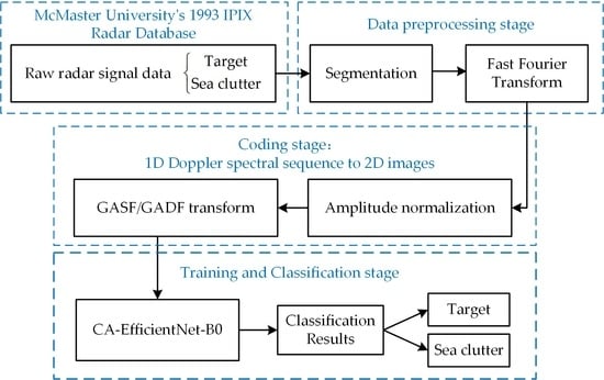
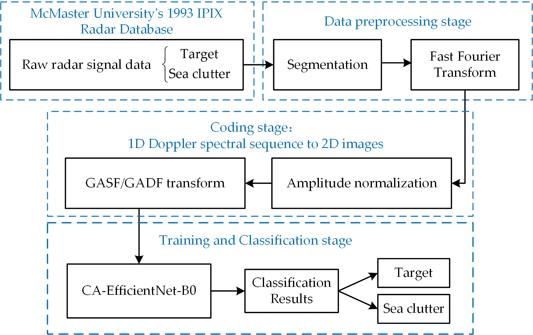
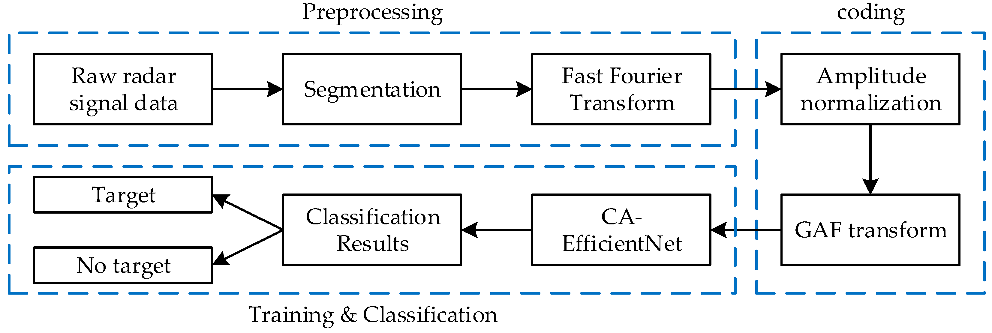
This study aims to propose a framework for classifying radar echo data using deep learning techniques. In this study, the raw radar echo data are first segmented, and then the segmented data are fast Fourier transformed to obtain the corresponding Doppler spectral sequence, followed by applying GASF and GADF to encode the Doppler spectral sequence into an image. Then, the transformed images are fed into the CA-EfficientNet-B0 network model incorporating the CA attention module for training, and finally the images to be detected are fed into the trained model for processing to identify the features in the images and perform classification.
This detection algorithm is divided into three main stages: (1) data preprocessing; (2) sequence coding; and (3) model training and prediction.
Figure 1 shows the block diagram of the improved EfficientNet-based algorithm for detecting small targets floating on the sea surface. The details of this algorithm are described in the subsequent subsections.
2.1. Data Description
The measured sea clutter data used in this paper come from the IPIX (Intelligent Pixel processing X-band) radar database website of McMaster University in Canada [
12]. The dataset was collected in 1993, measured with X-band fully coherent radar. The IPIX radar can transmit and receive electromagnetic waves of horizontal polarization (H-polarization) and vertical polarization (V-polarization) with center frequency of 9.39, peak power of 8, pulse repetition frequency (PRF) of 1 kHz, pulse width of 0.2, range resolution 30, and the number of pulses is 131072. Each group of data includes data of four polarization modes, VV, HH, VH and HV, and each polarization mode data includes echo signals of 14 range cells. The target is within one of the range cells, usually 2–3 range cells adjacent to the target cell are affected cells. The target is an airtight spherical container of diameter 1 wrapped in aluminum foil, capable of floating on the sea surface and moving randomly with the waves. The cell where the target is located is labeled as the primary target cell, the cell affected by the target is labeled as the secondary cell, and the rest of the cells are clutter-only cells. For ease of use, these 14 datasets are numbered and their file names, wind speeds, effective wave heights, primary target cells, and affected cells are listed in
Table 1.
2.2. Signal to Clutter Ratio Analysis
For the 14 sets of measured datasets in
Table 1, the SCR in short time intervals fluctuated around the Average SCR(ASCR) [
4]. Assuming that the target echo and sea clutter of the target cell are independent of each other, the ASCR of each dataset under any polarization can be calculated by the following equation [
13]:
where
represents the average power of sea clutter, estimated from the time series of all clutter cells of length 2
17.
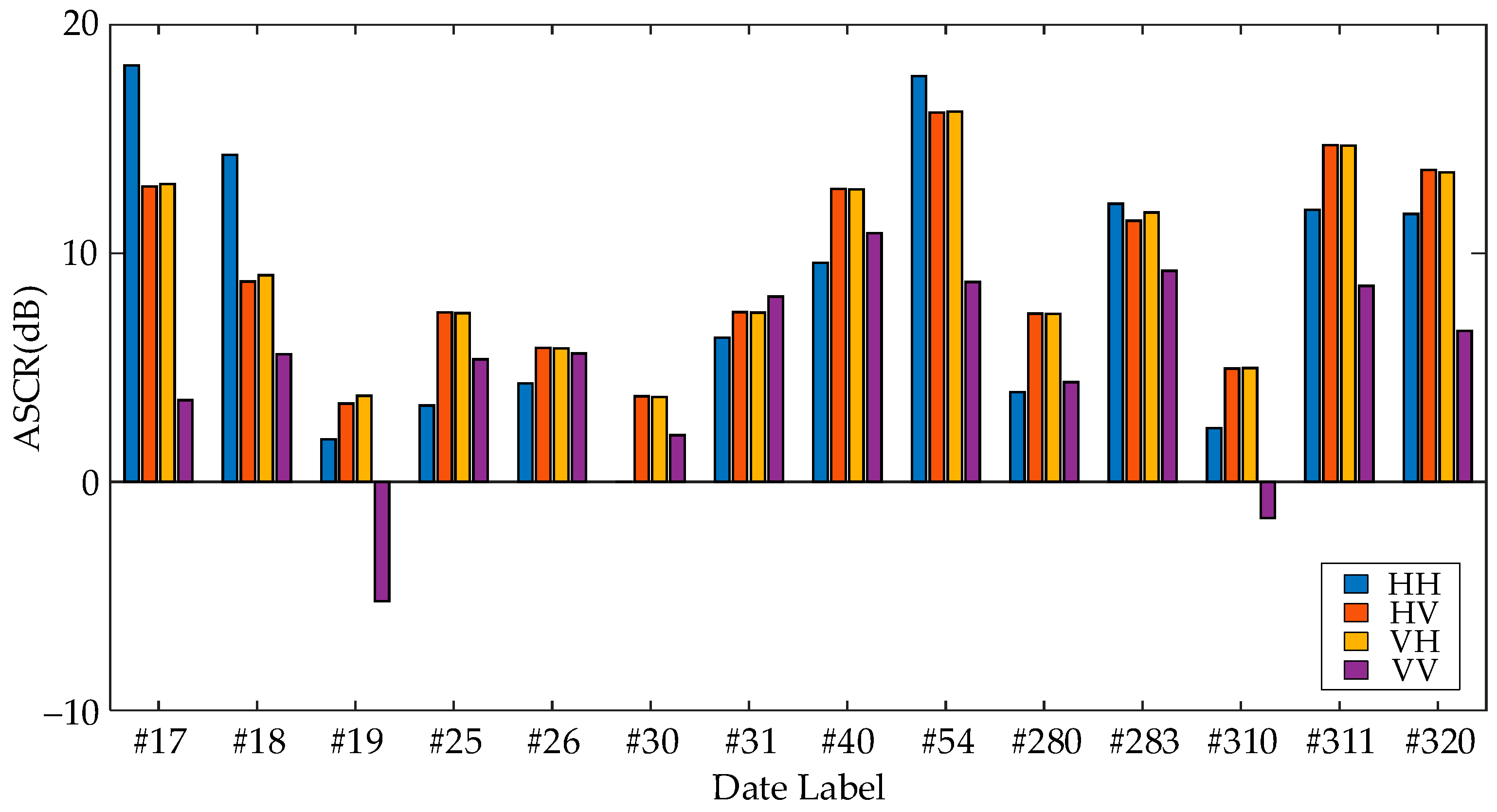
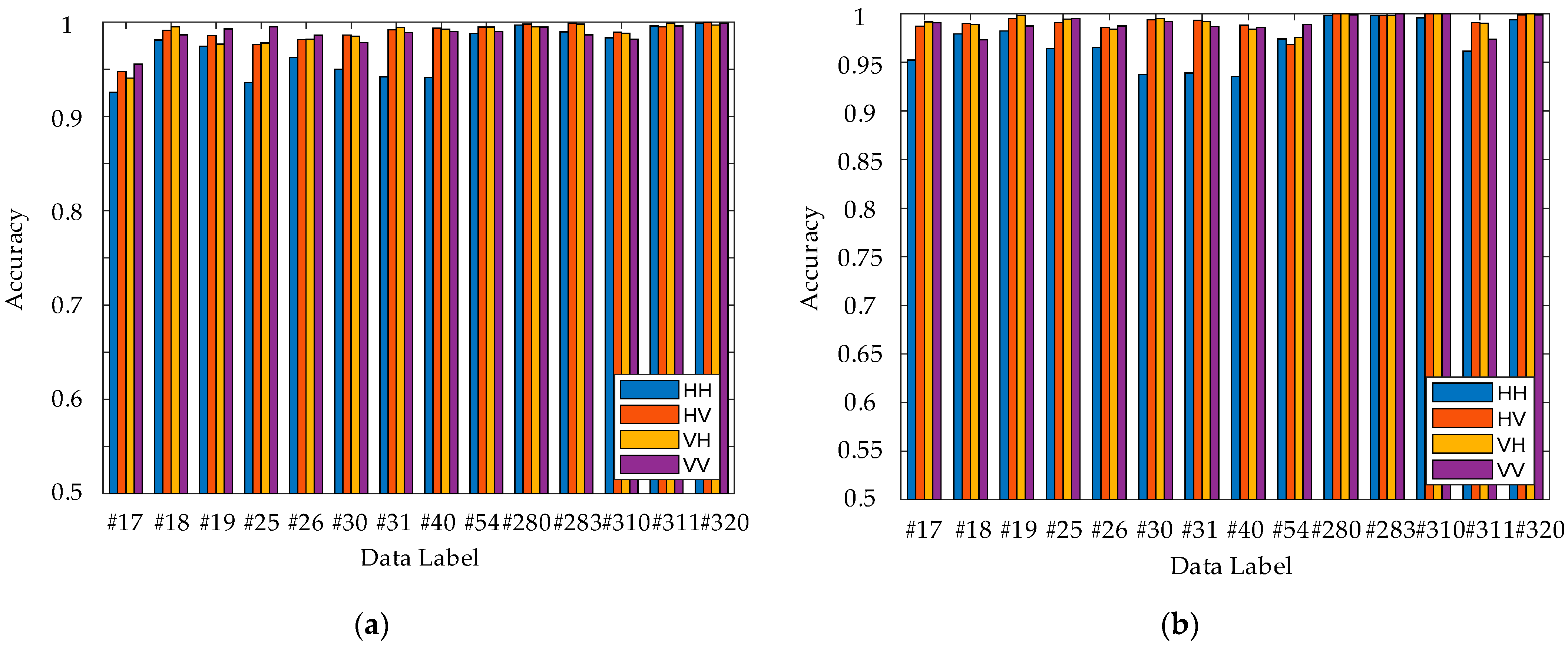
In this paper, we analyzed the ASCR of the target cell for 14 datasets under four polarization models, and the results are shown in
Figure 2. As can be seen from
Figure 2, the 14 datasets have completely different ASCR. In the same dataset, the radar echoes of HH, HV and VH polarization have higher ASCR than those of VV polarization, which is related to the clutter level under different polarization modes, the polarization characteristics of the target, the sea state and the radar-illuminated area of the target during the data acquisition. The ASCRs of the 14 datasets under the four polarization methods are distributed in the range of
, so these 14 datasets can be well used to measure the target detection performance of the proposed algorithm in this paper.
2.3. Analysis of Doppler Spectrum Characteristics
At each range cell, the received radar echo consists of the target, sea clutter, and noise. The echoes obtained by the IPIX radar can be divided into two categories: (1) If the measured range cell contains a target, the received echo consists of the target echo, noise, and sea clutter; (2) If the measured range cell does not contain a target, then the received echo contains only sea clutter and noise. At high SCR, the Doppler spectrum of target echo and sea clutter usually has an obvious difference: under the same sea condition, compared with sea clutter Doppler spectrum, the Doppler spectrum of target echo has stronger aggregation, lower central frequency, and more concentrated energy distribution.
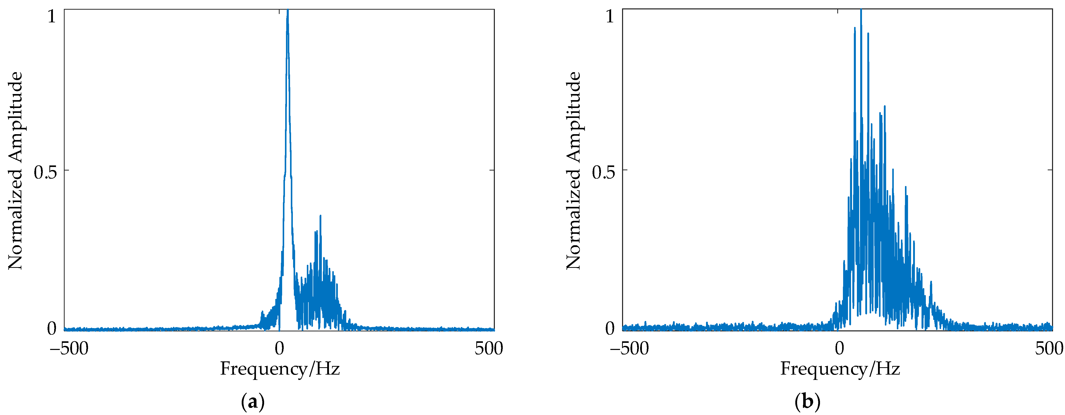
Taking the data file #280VV as an example, this paper selects cell 1 (sea clutter cell) and cell 8 (target cell) as a comparison, and splits the point sequence of each distance cell into 255 segments, with the length of each segment being 1024 and the overlap rate of two adjacent segments being 50%, and then performs 1024-point fast Fourier transform (FFT) and normalization on the segmented data to obtain its normalized Doppler spectrum as shown in
Figure 3.
From
Figure 3, it can be seen that the center frequency of the Doppler spectrum of both the target echo and the sea clutter is positive, which indicates that the ocean waves are moving closer to the radar. Compared with the target echoes, the sea clutter has a wider range of energy distribution in the frequency domain, this is because the ocean waves have more variable motion states and more complex scattering structures. In addition, although the motion state of the target will change with the change of sea state, the spatial geometry of the target is fixed, and the reflection of energy is more concentrated, so the Doppler spectrum of the target is more aggregated.
In fact, the differences between target echoes and sea clutter in the Doppler spectrum are not always as obvious as shown in
Figure 3, and target echoes and sea clutter often overlap highly in the time and frequency domains. Some statistical features proposed at this stage cannot fully describe the difference information contained in the Doppler spectrum of target echo and sea clutter, so the detection accuracy of the target in sea clutter by the one-dimensional method is not high. In order to exert the superior performance of deep learning in the field of image classification and target recognition, this study encodes the Doppler spectrum sequence of radar echo data into a two-dimensional image, and applies a CNN model to classify the transformed image.
2.4. Time Series Coding Methods
Inspired by the great success of deep learning in computer vision, Wang. et al. [
8] proposed two processing algorithms for encoding time series into images: GASF and GADF. These algorithms can convert a one-dimensional time series into a two-dimensional image, enabling the visualization of time series data. Meanwhile, the encoded image also retains the time dependence and correlation of the original data.
The GAF algorithm represents time series in polar coordinates rather than Cartesian coordinates, which evolved from the Gram matrix. The specific implementation of the steps of the GAF algorithm is as follows: Assuming that a time series
contains
n real-valued observations, we can rescale all the values of
X to the interval
by the normalization method shown in Equation (2):
Similarly, we can readjust all values of
X to the interval [0,1] using the normalization shown in Equation (3):
We denote the rescaled time series as
and then map
to polar coordinates using the following equation:
where
represents the arc cosine of
, corresponding to the angle in the polar coordinate system,
represents the polar coordinate radius corresponding to the timestamp
, and
plays the role of adjusting the span of the polar coordinate system.
The scaled data of the two normalization operations correspond to different angle ranges respectively when converted to the polar coordinate system. The data within the range of
corresponds to the arc cosine function angle range of
, and the arc cosine value range corresponding to the data in the range of
is
. This polar coordinate system-based representation provides us with a new perspective for understanding time series, that is, the timescale changes of the series are mapped to the radius of the polar coordinate system over time, while the amplitude changes are mapped to the angle of the polar coordinate system. By calculating the sum and difference of trigonometric functions between sampling points, GASF and GADF are respectively defined as follows:
In summary, the GAF algorithm is used to convert the one-dimensional time series into a two-dimensional image through three steps: scaling, coordinate system conversion, and trigonometric function operations.
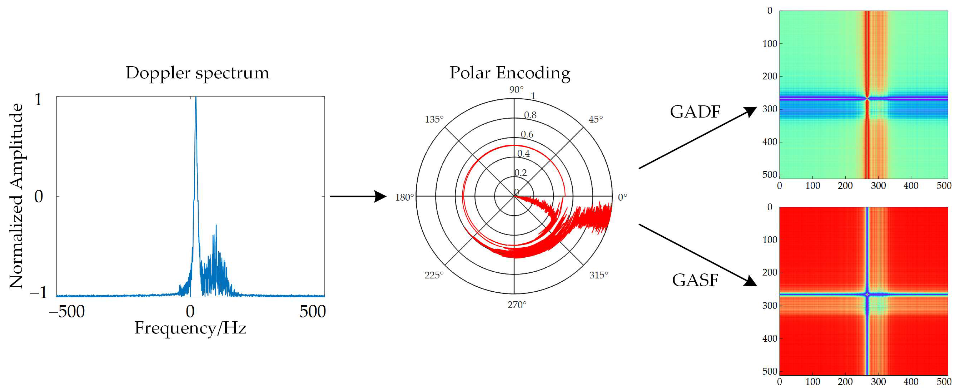
Figure 4 shows the complete process of converting the rescaled Doppler spectrum sequence into a GAF-encoded map. First, the Doppler spectral sequence is normalized using Equation (2); then the normalized Doppler spectral sequence is converted to a polar coordinate system for representation using Equation (4); finally, the data matrices of the GASF and GADF images are obtained using Equations (5) and (6), respectively.
2.5. CA-EfficientNet Network Model
To obtain better accuracy for network models, optimization of network depth, network width, and image resolution is usually adopted, such as ResNet [
14], DenseNet [
15], etc. However, these network models often change only 1 of the 3 dimensions of network depth, network width, and image resolution, and require tedious manual adjustment of parameters, and still yield sub-optimal accuracy and efficiency. In 2017, Google proposed depthwise separable convolution (DSC) as the basis for building the lightweight network MobileNet [
16], which also allows users to modify the two parameters of network width and input resolution to adapt to different application environments; in 2019, Google Brain Team proposed the EfficientNet network model, which takes into account the depth, width, and resolution of the input image without increasing the number of parameters and operations, and scales these three parameters reasonably and efficiently to achieve optimal accuracy.
2.5.1. EfficientNet Model Selection
Compared with other network models, the EfficientNet family of networks can maintain high classification accuracy with a small number of model parameters at the same time. The scale of the network model is mainly determined by the scaling parameters in three dimensions: width, depth, and resolution. The higher the resolution of the input image, the deeper the network is needed to obtain a larger perceptual field of view, and similarly, the more channels are needed to obtain more accurate features. A total of eight models from B0 to B7 are constructed for the EfficientNet network according to the image resolution. The size of the B0~B7 model increases sequentially with higher accuracy and greater memory requirements. Among them, the accuracy of the B7 model is 84.4% and 97.1% for Top-1 and Top-5, respectively, on the natural image ImageNet dataset, which has reached the best accuracy at that time. The B0~B7 models have the least number of operations among the networks that achieve the same accuracy.
For the characteristics of GAF images, we expect the selected base network model to have strong feature extraction capability and high recognition accuracy. We also need to consider the hardware implementability of the network, which requires that the number of parameters of the network model should not be too large. Higher image resolution can show more texture details, which is beneficial for the improvement of recognition accuracy. As the image resolution increases, the time and memory required to train the network model also increases exponentially. In order to select a suitable structure from the EfficientNet family of networks as our base network, we conducted comparison experiments on different network structures on the generated GADF and GASF datasets, respectively. We trained the network with the number of iterations set to 100 and the initial learning rate of 0.001, and the experimental results on the validation set are shown in
Table 2.
From
Table 2, we can see that the computational effort increases exponentially as the complexity of the network model increases, which is manifested by a geometric increase in training time. The classification results on the GADF and GASF validation datasets do not improve with the increase of the complexity of the network. The accuracy of the B7 network model based on GADF validation datasets is higher than that of the B0 network model by 0.03%, and the accuracy of the B7 network model based on GASF validation datasets is higher than that of the B0 network model by 0.06. The accuracy of all other models is lower than that of the B0 network model. Therefore, we chose EfficientNet-B0, which has the least model parameters and the fastest training speed, as the base network for the next step.
The network structure of EfficientNet-B0 is shown in
Table 3, which consists of 16 MBConv blocks, 2 convolutional layers, 1 global average pooling (GAP) layer, and 1 fully connected layer. The MBConv block contains the Depthwise (DW) Convolution, Squeeze-and-Excitation (SE) attention mechanism module, Swish activation function, and Dropout layer. The SE module compresses the input 3D feature matrix into a one-dimensional channel feature vector by a global average pooling operation, which reflects the importance of different channels of the input feature matrix.
2.5.2. Coordinate Attention
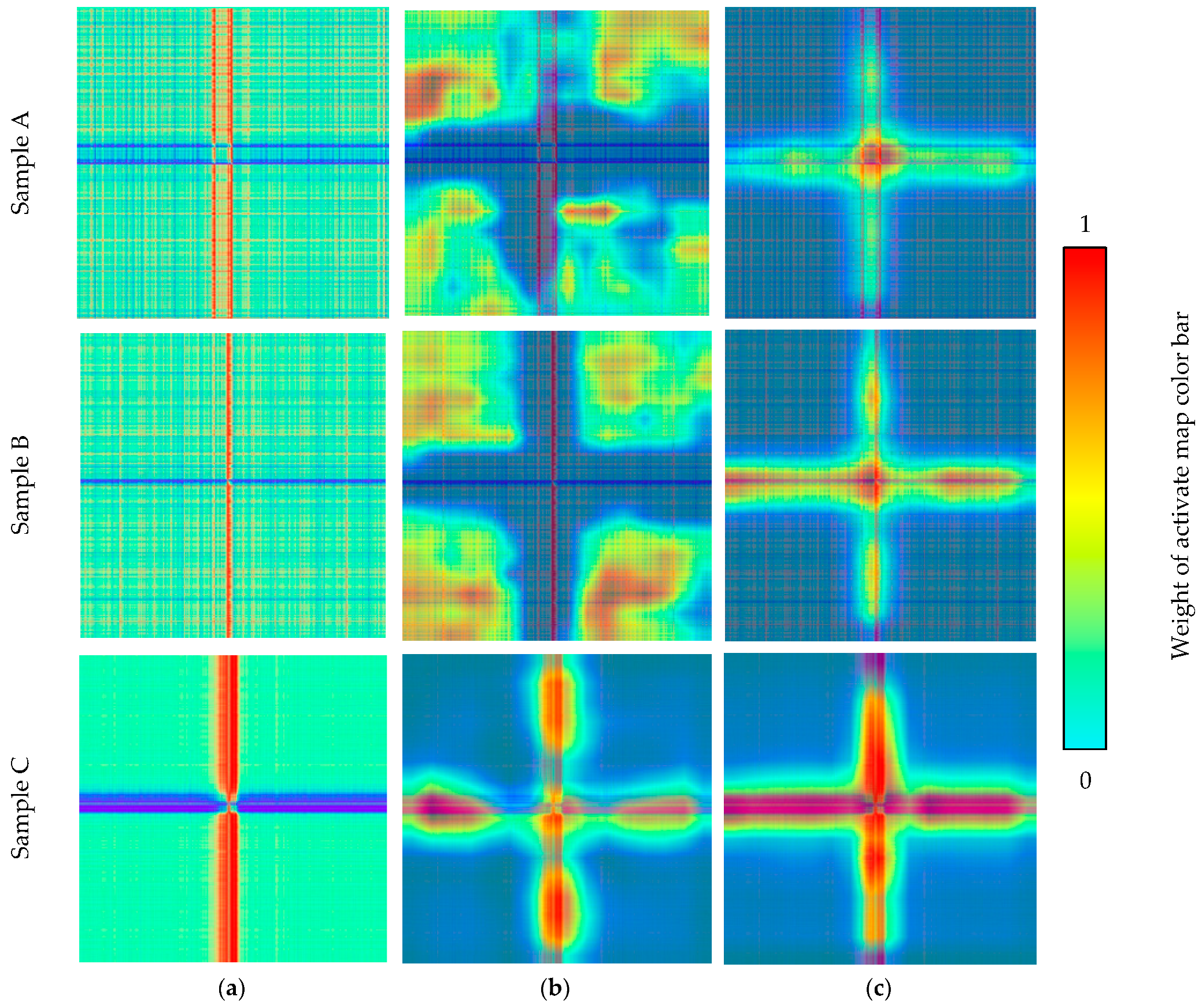
We conducted an observational study on a large sample of both coded maps and found that the texture features of the target and sea clutter are not randomly distributed. These texture features will only appear in specific regions, while most of the remaining regions will have duplicate texture information and no texture information. The focus on these regions with duplicated textures and regions without texture may be ineffective, so we need to emphasize the location information in the coded maps that is critical for target identification.
The channel attention mechanism has a significant effect on improving the model performance, but it only focuses on the long-term dependencies between channels and ignores the importance of location information. A new network attention mechanism is proposed in the literature [
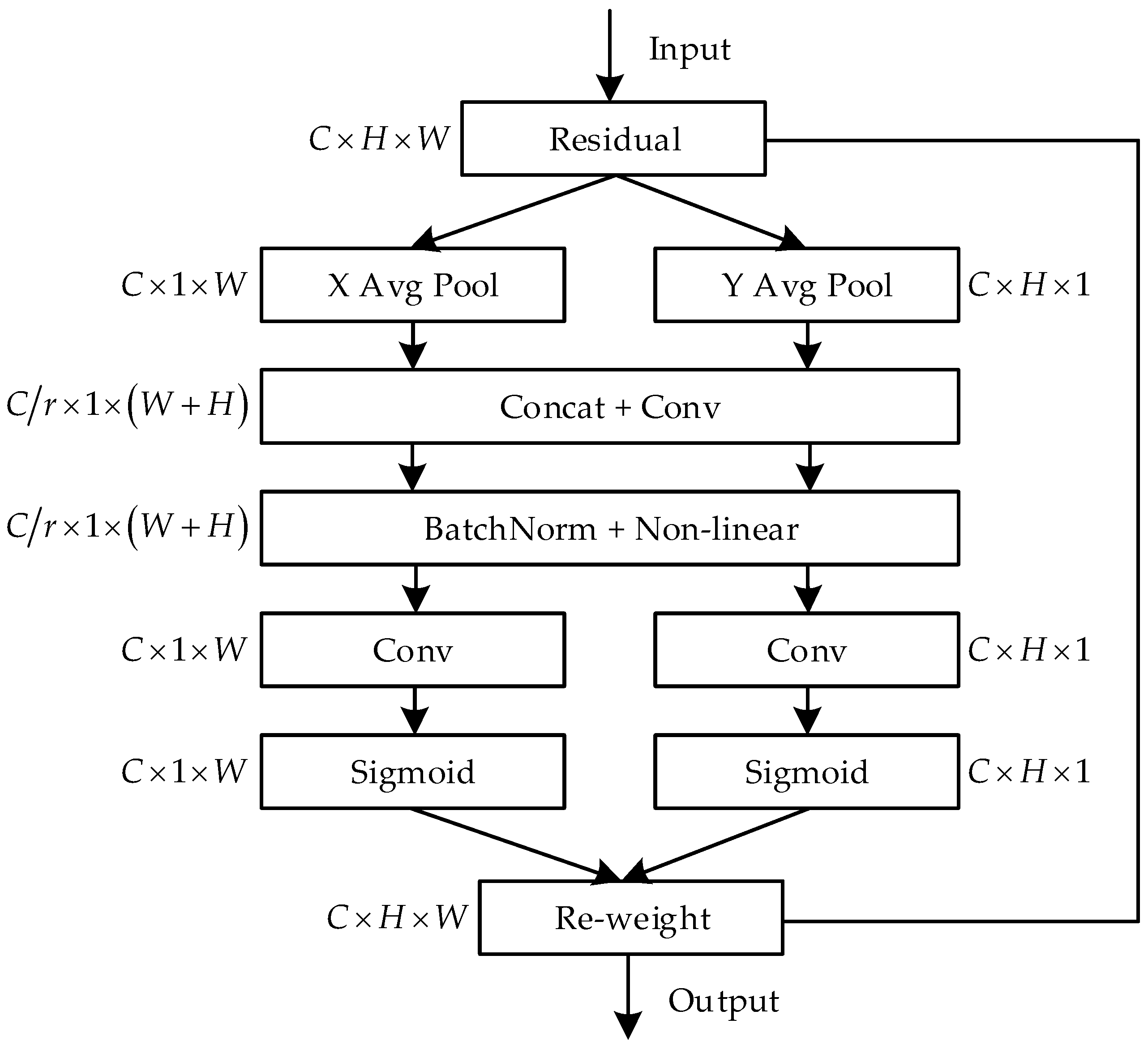
11], which embeds location information into channel attention, called the coordinate attention mechanism. Unlike channel attention that transforms feature tensor into a single feature vector, the coordinate attention mechanism decomposes channel attention into two one-dimensional feature encoding processes that aggregate features along two spatial directions, respectively. In this way, long-term dependencies are captured so that channel dependencies can be obtained while retaining precise location information. The generated feature maps are then encoded into direction-aware and position-aware attentional feature maps, respectively. This pair of attentional maps can be complementarily applied to the input feature maps to increase the representation of the object of interest. The coordinate attention mechanism is relatively simple and computationally small and is easy to insert into the network structure. A structure diagram of the CA module is shown in
Figure 5.
2.5.3. Improvement of EfficientNet
To further improve the recognition accuracy of the sea clutter target detection model, this study introduces CA to further improve EfficientNet to enhance the learning of location information that plays an important role in the coded graph. Compared with the original EfficientNet network model, the following improvements to the network model are mainly made in this study.
Connecting CA modules in the form of residual structures after the first convolutional layer of the network. This is because the CA module changes the weight parameters by combining the features of the convolutional layers, applying larger weights to the important feature channels and smaller weights to other less important feature channels. The CA module enhances the global attention of the CNN so that the network does not lose more critical information due to the pre-convolutional operation, thus improving the model’s ability to distinguish between targets and sea clutter.
The SE module within each MBConv module in the original EfficientNet network is replaced with a CA module. Specifically, for the MBConv module structure shown in
Figure 6, the original SE module after the DW convolution module in it is replaced with a CA module. By this operation, the CA module can be used to capture the long-term dependency between network channels, so that the network can pay attention to the target-relevant region without losing the accurate position information.
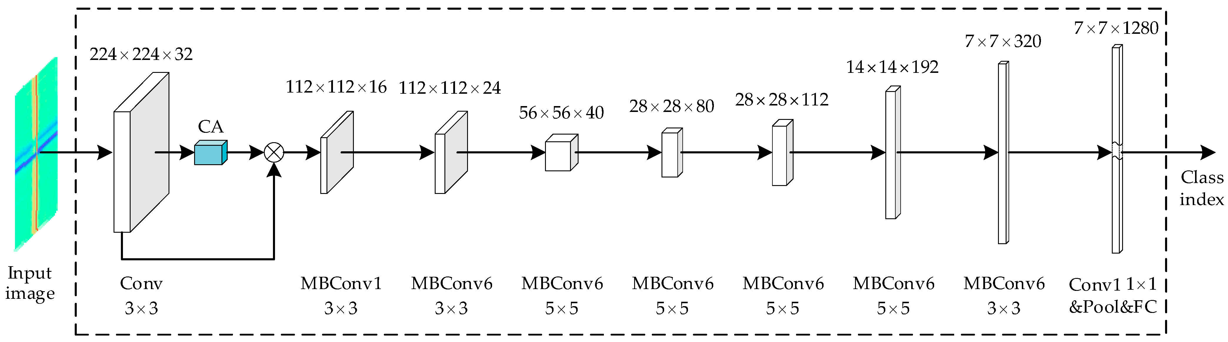
The structure of the improved CA-EfficientNet-B0 network is shown in
Figure 7: first, the input image is converted into a
matrix; then, the feature map after the first layer of the convolution operation is multiplied with the attention feature map enhanced by the CA module at the channel level to obtain the feature map with attention information; then, the higher-level features of the image are further extracted by seven MBConv modules embedded with CA in turn to obtain the 7 × 7 × 1280 feature map; finally, the result of the image recognition is obtained by the fully connected layer.
3. Results
3.1. Construction of Training Dataset
The data used for model training and testing were converted from the measured sea clutter data. The 14 sets of measured data listed in
Table 1 were converted into the corresponding two types of datasets according to the GASF and GADF coding methods mentioned in
Section 2.4, respectively. First, the data of each distance cell are partitioned into subsequences of a length of 1024, and the interval overlap of adjacent subsequences is 50%. Then, the Doppler spectra of corresponding subsequences are calculated using 1024-point FFT, and then the normalized Doppler spectral sequences are encoded into GASF maps and GADF maps, respectively. Finally, they are used to construct the two datasets, respectively. We selected 85,680 images from the existing coding library for our test and validation sets, including 42,840 images for GADF and GASF, with a 4:1 ratio of training to validation and a 2:1 ratio of clutter to target. A total of 57,120 images were selected for the test set, including 28,560 images for GADF and GASF, with a 1:1 ratio of clutter to target.
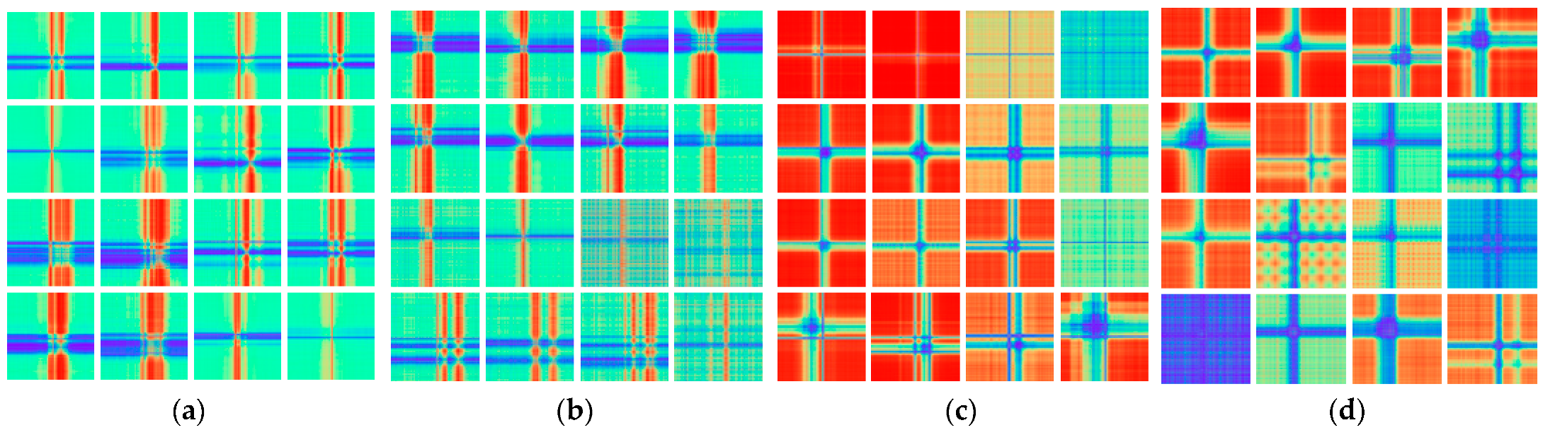
Figure 8 shows the sample of GADF and GASF coded images corresponding to the target and clutter in the dataset.
3.2. Experimental Environment and Parameter Settings
All training and testing experiments were performed on the Linux operating system, and the open source Pytorch deep learning framework was used to build the network model. The CPU was AMD EPYC 7543 32-Core Processor with 30 GB of RAM, and the GPU was RTX A5000 with 24 G of video memory. The programming language was Python3.8, and the integrated development platform was PyCharm2021.1.3. In each batch, 64 images were trained, the iteration period was 100 times, the initial learning rate was set to 0.001, the AdamW optimizer was chosen to optimize the model parameters, the learning rate was adjusted by the cosine annealing algorithm strategy, the learning rate was adjusted from the initial learning rate to 0 within 100 epochs, and the loss function was the SoftMax cross-entropy loss function.
3.3. Test Evaluation Indicators
In order to evaluate the classification performance of the CA-EfficientNet-B0 network model proposed in this paper, the recognition accuracy (Accuracy), F1 value, number of parameters, and Floating-Point Operations (FLOPs) are selected as evaluation metrics in this study. The number of parameters is the total number of parameters that can be trained in the network model, measured in millions (M). The FLOPs are the number of floating-point operations, and are used to measure the complexity of the algorithm or model, and are measured in billions (B). The recognition accuracy is the probability value of the number of correctly predicted samples to the total number of tested samples. For image classification network models, recognition accuracy is the most important evaluation index, and its calculation formula is as follows:
where
denotes the number of correctly predicted samples and
denotes the total number of samples in the test set. To comprehensively evaluate the performance of the CA-EfficientNet model, this study also used the value that considers both the accuracy and recall of the classification model, which is calculated as follows:
where Precision is the accuracy rate, which indicates how many of the totally predicted positive samples in the test set were correctly predicted; Recall is the recall rate, also called the full rate, which indicates how many of the positive samples in the original total positive sample sets were correctly predicted. The precision and recall rates are calculated as follows:
where TP, FP, TN, and FN represent the number of true positive, false positive, true negative, and false negative samples, respectively.
3.4. Training and Testing
For the CA-Efficient network model proposed in
Section 2.5, the model was trained using the experimental setup given in
Section 3.2. The training loss and validation loss curves are shown in
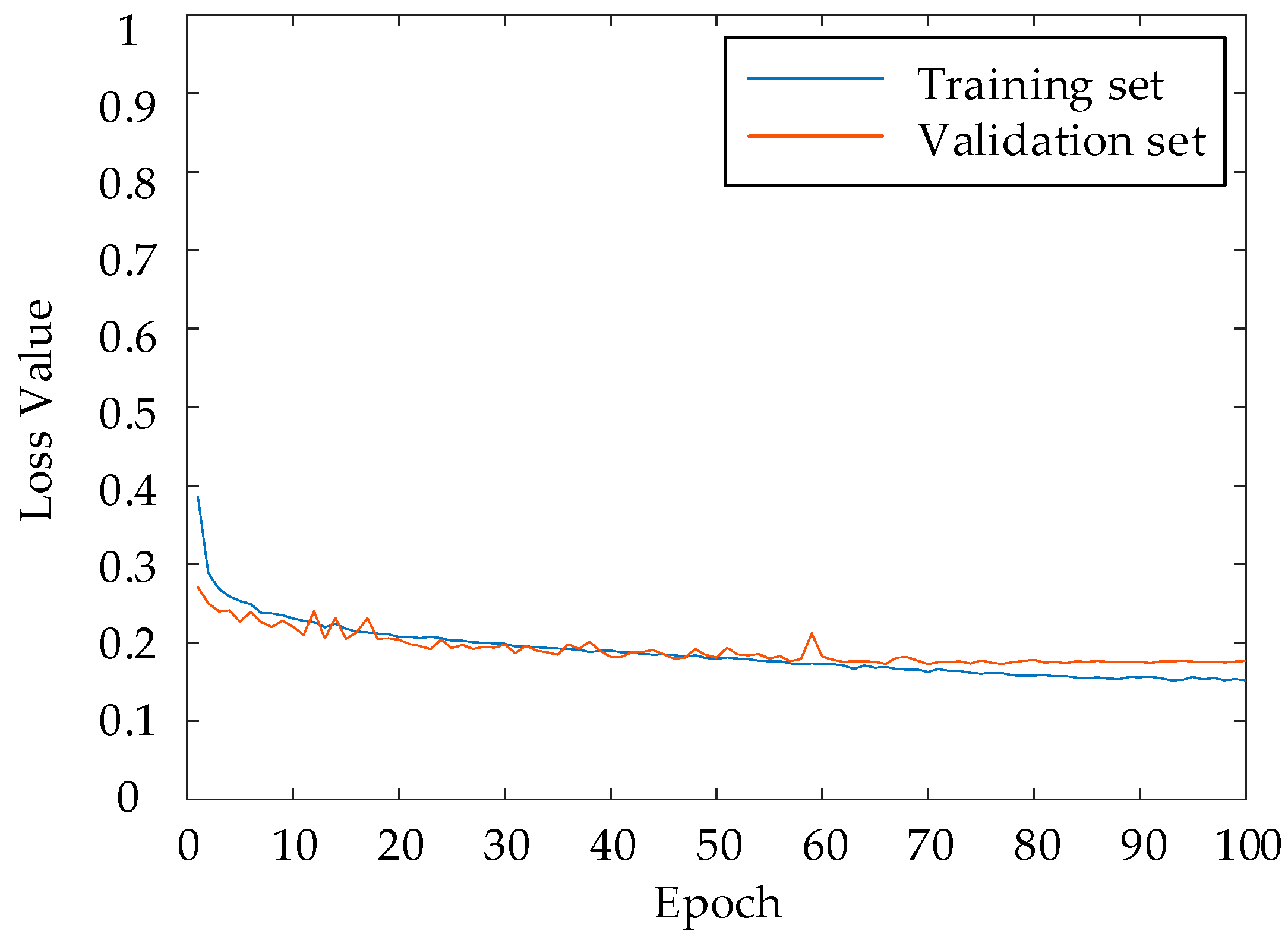
Figure 9. From the figure, it can be seen that the training and validation loss values can drop steadily and quickly with the increase in the value of the epoch. It indicates the effectiveness and learnability of the model. At iteration number 70, the validation loss value was close to convergence and the classification accuracy tended to be stable. The training loss value basically converged at the 90th iteration, indicating that the model reached saturation and the recognition accuracy no longer increases. This indicates that the experimental setup of this study is reasonable and feasible.
3.5. CA-EfficientNet Model Ablation Trials
In order to verify the effectiveness of the CA-EfficientNet-B0 model proposed in this study, four ablation test schemes were used in this study as follows.
Scheme 1: Using EfficientNet-B0 only, with the optimizer choosing stochastic gradient descent (SGD) + momentum and the learning rate adjustment strategy choosing cosine annealing algorithm.
Scheme 2: Replacing the optimizer with the AdamW optimization algorithm on the basis of Scheme 1.
Scheme 3: Replacing the SE module of the MBConv module in the EfficientNet-B0 network with the CA module on the basis of Scheme 2.
Scheme 4: Based on Scheme 3, the CA module is introduced after the first convolutional layer to form the lightweight network model CA-EfficientNet-B0 proposed in this study.
The experimental results of the above ablation test schemes are shown in
Table 4. From the experimental results of Scheme 1 and Scheme 2, it is clear that the AdamW optimizer can robustly improve the convergence of the model. Comparing the experimental results of Scheme 2 and Scheme 3, it is clear that the CA module has stronger attention learning ability than the SE module. Comparing the experimental results of Scheme 3 and Scheme 4, it is clear that adding the CA module after the first module is effective. From the experimental results of Scheme 4, it can be seen that the improved CA-EfficientNet-B0 model proposed in this study achieves 96.13% and 96.28% recognition accuracy on the GADF and GASF test datasets, respectively. Compared with the baseline model, the accuracy of the improved network model proposed in this study was improved by 1.74% and 2.06% on the GADF and GASF datasets, respectively. The combined experimental results of Schemes 1, 2, 3, and 4 show that the model improvement scheme and the network training strategy in this study are feasible and effective. In summary, the CA-EfficientNet-B0 model is a lightweight and deep network model with good recognition accuracy.
5. Conclusions
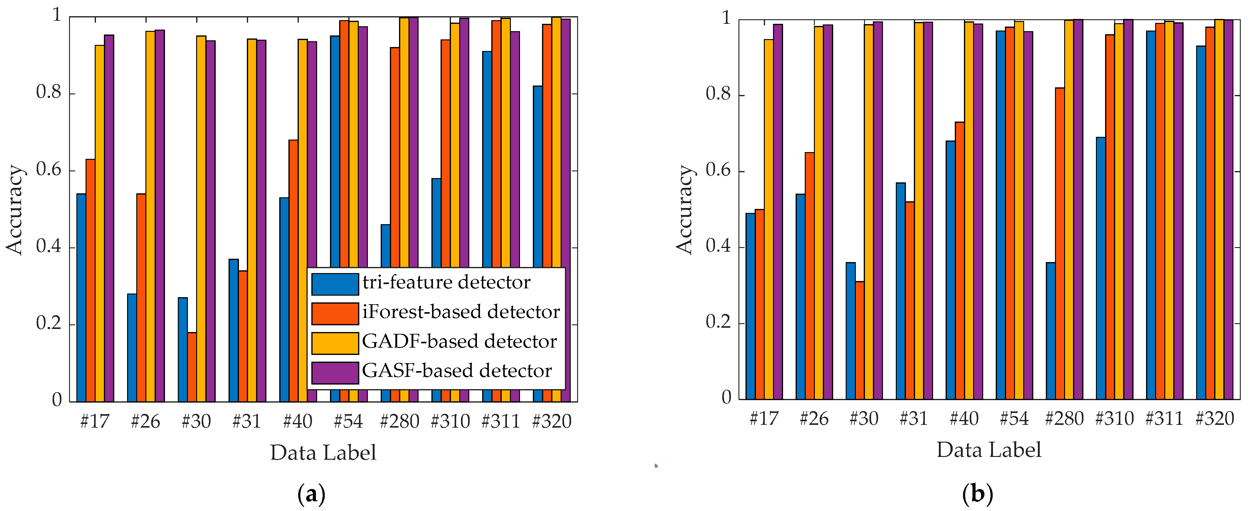
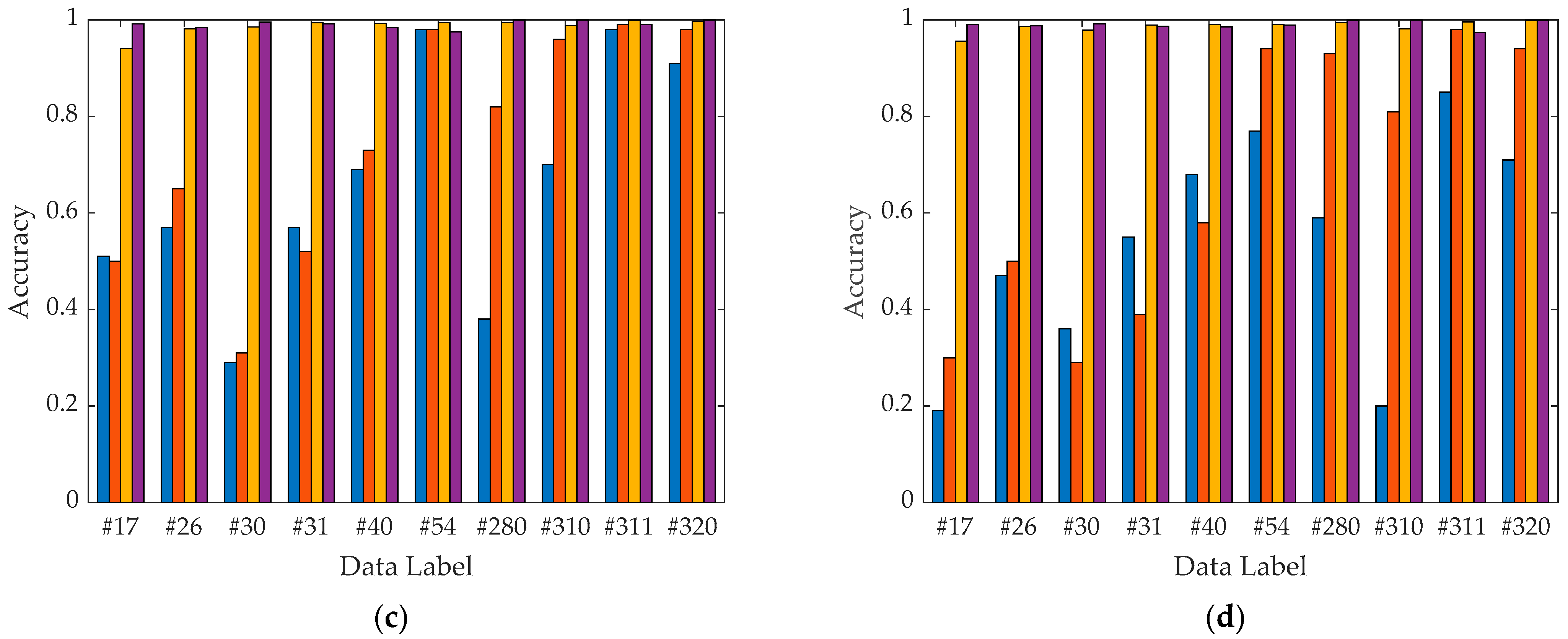
In this paper, we convert the target recognition problem into a classification problem for Doppler spectral encoded maps. We use the improved CA-EfficientNet-B0 model to train and test the experimentally generated dataset for the detection of targets on the sea surface. The detection and classification results show that the CA-EfficientNet-B0 network model proposed in this paper has the advantage of high accuracy and intelligence in the detection of small floating targets on the sea surface, and our method is effective in the classification of both targets and clutter. In addition, by comparing with other classical classification algorithms, it is shown that the CA-EfficientNet-B0-based method proposed in this paper has more advantages in detection and recognition probability, and also provides a new idea for radar sea moving target detection and classification. Both the proposed GADF and GASF coded graph detection methods have good recognition performance, and for the same Doppler spectral sequence, the two coding methods exhibit different characteristics. It leads to the datasets constructed based on the two coding methods exhibiting different detection performance in the same network model, and the average detection accuracy of the dataset based on the GASF coding method is higher than that of the GADF coding method based on the datasets.
Since there are some differences in the description and details of the same Doppler spectral sequence between GASF and GADF coding, how to fuse the two different coding methods and apply them to the deep learning model is a problem that needs to be solved in the future. In addition, finding a more suitable time series coding algorithm for this research and further improving the detection accuracy of the network model are also the future exploration directions of this research.


