Establishment and Extension of a Fast Descriptor for Point Cloud Registration

Abstract

Point cloud registration (PCR) is a vital problem in remote sensing and computer vision, which has various important applications, such as 3D reconstruction, object recognition, and simultaneous localization and mapping (SLAM). Although scholars have investigated a variety of methods for PCR, the applications have been limited by low accuracy, high memory footprint, and slow speed, especially for dealing with a large number of point cloud data. To solve these problems, a novel local descriptor is proposed for efficient PCR. We formed a comprehensive description of local geometries with their statistical properties on a normal angle, dot product of query point normal and vector from the point to its neighborhood point, the distance between the query point and its neighborhood point, and curvature variation. Sub-features in descriptors were low-dimensional and computationally efficient. Moreover, we applied the optimized sample consensus (OSAC) algorithm to iteratively estimate the optimum transformation from point correspondences. OSAC is robust and practical for matching highly self-similar features. Experiments and comparisons with the commonly used descriptor were conducted on several synthetic datasets and our real scanned bridge data. The result of the simulation experiments showed that the rotation angle error was below 0.025° and the translation error was below 0.0035 m. The real dataset was terrestrial laser scanning (TLS) data of Sujiaba Bridge in Chongqing, China. The results showed the proposed descriptor successfully registered the practical TLS data with the smallest errors. The experiments demonstrate that the proposed method is fast with high alignment accuracy and achieves a better performance than previous commonly used methods.

1. Introduction

In recent years, the research of computer vision and autonomous driving has received more and more attention. Three-dimensional rigid PCR is a basic and critical problem in the field of 3D vision, such as 3D modeling [1,2], localization for robot navigation [3,4,5], object recognition [6,7,8], and surface alignment [9,10]. The purpose of PCR is to seek the best transformation parameters that precisely aligns a pair of point in different coordinate systems.

The iterative nearest point (ICP) algorithm is the most commonly applied PCR method because the iteration is simple, and the convergence speed is fast [11,12,13,14]. It iteratively calculates the optimum transformation until the function criterion converges to the specified value. Unfortunately, the ICP algorithm is susceptible to local minima [15], so good initialization is required to obtain satisfactory registration results. Therefore, the common practical solution is the “coarse to fine” strategy [16,17,18]; that is, a good initial position is obtained by using the coarse registration, and then the ICP algorithm can achieve an accurate alignment with a fast speed. Due to the original point cloud with unknown orientations, coarse registration isis a challenging task and has attracted increasing attention in the past few years. Our proposed algorithm belongs to the coarse registration category. Generally, we categorize the coarse registration algorithms based on global features [19] and local features [20]. The shape contexts [21] and extended Gaussian images [22,23] methods which belong to global feature descriptors, have the advantage of rotation invariance. Considering the complexity of the descriptor and memory footprint, the methods based on local features are generally efficient in aligning the source and target point clouds [24,25,26,27]. Therefore, we mainly focus on the PCR method based on local features.

To date, the point pair feature (PPF) descriptor is the classical method for local surface description [28]. Johnson and Hebert [29] designed spin image (SI) features, and the local reference axis (LRA) is created by using 3D points with relevant directions. Then according to the correlation coefficient of SI, the matching point pairs are established. Although SI is one of the most commonly cited methods, it is highly disturbed by the data resolution. The point feature histogram (PFH) descriptor has the advantages of high discriminatory and descriptive power but is extremely time-consuming [30]. Then to solve the problem, the fast point feature histogram (FPFH) [31] descriptor is proposed by calculating the normal angle, weighting, and summing the features. It significantly accelerates the PCR speed. The signature of histograms of orientations (SHOT) [32] method first establishes LRA. Then dataset is fixed to LRA and is divided into different blocks. The deviation angle of normal is summed in each block. Finally, the SHOT feature is obtained by concatenating all the histograms. The SHOT method achieves good performance in terms of efficiency, discrimination, and robustness [33]. The rotation projection statistics (RoPS) feature descriptor is one of the best-performing feature descriptors in feature matching. This method mainly consists of three processing steps: LRF definition [34], RoPS feature construction, and 3D object recognition. The eigenvalue decomposition of the scatter matrix formed three eigenvectors. Then the LRF establishment is based on the eigenvectors. Triple orthogonal local depth images (TOLDI) [35] is a relatively new feature descriptor, three orthogonal depth maps of a specified point are obtained by projection discretization. The pixel values of depth mapping are directly spliced as a description of a specified point.

As mentioned above, the researchers have conducted detailed studies on the coarse registration algorithm based on feature descriptors. Feature-based methods do not rely on the initial pose, while good features will speed up the registration and improve the accuracy of PCR. With the development of 3D scanner technology, the point cloud is more and more convenient to acquire, and the capacity of data is large. Due to the large capacity of point clouds, the dimension of feature, storage overload, and calculation cost is extremely high. Meanwhile, wrong matching point pairs will occur because of self-similar features derived from low-dimensional information [36]. In this paper, we analyze some typical local features and integrate them into a new descriptor. Specifically, we use the geometric features brought by normal information, dot product of normal and vector from specified point to its neighborhood point, distance parameter, and curvature variation. We validate our proposed method by conducting a comparison with popular methods on synthetic and real scanning datasets. Experimental results show that the proposed registration method based on the new descriptor has higher registration accuracy, fast calculation speed, and low memory footprint. To summarize, the main contributions of the proposed method are as follows:

(1)

We analyze some typical local invariant features and integrate them into a new descriptor. The proposed descriptor is highly descriptive. It contains rich information by considering angle, dot product, distance, and curvature characteristics.

(2)

Our method maintains a high registration accuracy with fast speed and low memory footprint. Besides the original point cloud, only the 32-D descriptor is stored in the memory. Hence, the proposed descriptor is time and memory efficient.

(3)

The new method can process directly on the scattered point clouds, which do not require any prior information. It does not need error preprocessing steps which are time-consuming.

The remainder of this paper is structured as follows. In Section 2, we introduce the proposed feature descriptor and present the details of the registration method based on the novel descriptor. We present the detailed description of experiment data in Section 3. The results and comparisons are given to test the accuracy, effectiveness, and efficiency of the proposed method, and we also discuss our results in Section 4. Finally, we draw conclusions in Section 5.

2. Methodology

The proposed method in this paper mainly consists of four steps. First, the source and target point clouds are simplified to 3D key points using the voxel grid method. We present the local descriptor of 3D key points for feature description. Then, point correspondences are established via feature matching. Finally, we utilize the OSAC algorithm to eliminate false matching point pairs. A good alignment position is obtained by using coarse registration.

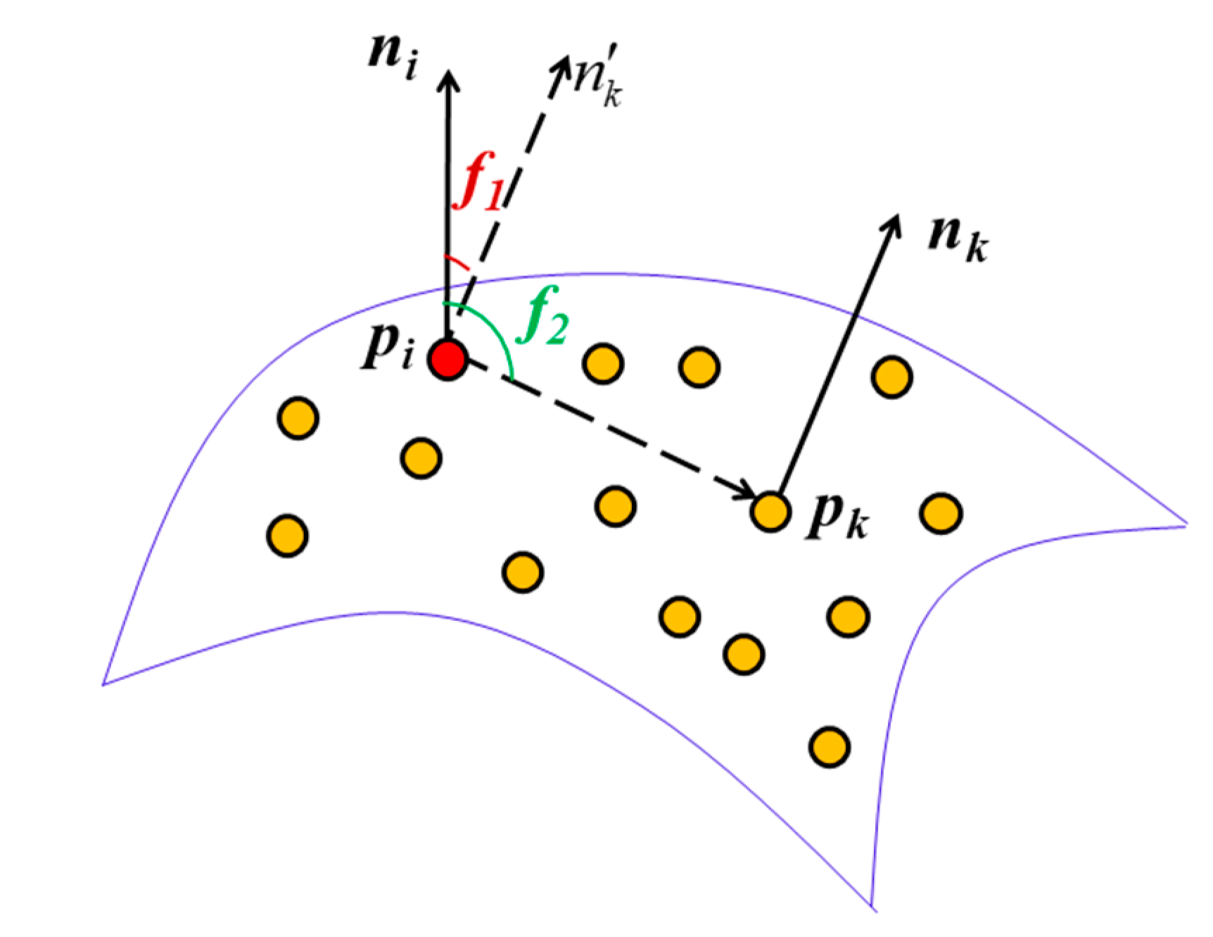
2.1. Definition of Descriptor

Local feature-based methods for 3D registration align a pair of point clouds by using point correspondences. The correspondences are usually obtained via matching feature descriptors. Hence, in order to acquire a sufficient number of correct matching correspondences, the feature descriptor should be descriptive, robust, and distinctive. More importantly, it should be invariant to rigid transformation. In this chapter, we briefly introduce a novel local feature descriptor by calculating the statistics of local invariant features.

Geometric features such as normal vector, distance parameter, and curvature variation reflect the most basic geometry of the point cloud. They are vital to express the local features of the point cloud. In addition, these specific features are invariant features with rotation or translation. They are distinctive to allow for effective description and are easy to calculate. We propose the use of a better system that combines several aspects of the geometry of a point’s neighborhood for estimating a multi-value feature set.

The feature description proposed in this paper is mainly divided into four steps: (1) calculating the normal angles, (2) calculating the dot product, (3) calculating the distance between the specified point and neighborhood points, and (4) calculating curvature variation. Figure 1 shows the schematic of the proposed method.

2.1.1. Angle between Normals

Previous studies have shown that the angle between a pair of normals has a high discriminative power [37]. To calculate the normal vector, we use the method in literature [38]. A brief introduction is as follows. The covariance matrix C for a data point p is given by,

$$C={\left[\begin{array}{c}{p}_{i_1}-\overline{p}\\ \dots \\ p_{i_k}-\overline{p}\end{array}\right]}^T\cdot \left[\begin{array}{c}{p}_{i_1}-\overline{p}\\ \dots \\ p_{i_k}-\overline{p}\end{array}\right],i_j\in N_p$$

(1)

where $\overline{p}$ is the centroid of the neighborhood point $p_{i_j}$ of point p.

Considering the eigenvector problem, Equation (1) can be expressed as follows,

$$C\cdot {\overrightarrow{v}}_l={\lambda }_l\cdot {\overrightarrow{v}}_l,l\in \left\{0,1,2\right\}$$

(2)

The eigenvalues ${\lambda }_0,{\lambda }_1$ and ${\lambda }_2$ of $C$ and the unit eigenvectors ${\overrightarrow{e}}_0,{\overrightarrow{e}}_1$ and ${\overrightarrow{e}}_2$ are calculated. Note that the vector ${\overrightarrow{e}}_0,{\overrightarrow{e}}_1$ and ${\overrightarrow{e}}_2$ are normalized vectors from ${\overrightarrow{v}}_0,{\overrightarrow{v}}_1$ and ${\overrightarrow{v}}_2$, respectively. The eigenvector corresponding to the minimum eigenvalue of $C$ is defined as the normal of p.

Given a query point $p_i$, the points in the sphere with radius r excluding $p_i$ are the neighborhood point of $p_i$. We suppose $p_k$ is the neighborhood point of $p_i$. The normal direction of $p_i$ and $p_k$ is ${\overrightarrow{n}}_i$ and ${\overrightarrow{n}}_k$, respectively. The cosine of the normal angle between ${\overrightarrow{n}}_i$ and ${\overrightarrow{n}}_k$ can be expressed as follows.

$$\cos {\theta }_{{\overrightarrow{n}}_i{\overrightarrow{v}}_k}=\frac{{\overrightarrow{n}}_i\cdot {\overrightarrow{n}}_k}{\left|{\overrightarrow{n}}_i\right|\left|{\overrightarrow{n}}_k\right|}$$

(3)

where the value range of ${\theta }_{{\overrightarrow{n}}_i{\overrightarrow{n}}_k}$ is [0, 180°]

The ${\theta }_{{\overrightarrow{n}}_i{\overrightarrow{n}}_k}$ is defined as $f_1$ in this paper. The sub-feature $f_1$ is mainly distributed between 0° and 60° in most cases. Hence it is divided into four intervals (0°, 20°), (20°, 40°), (40°, 60°), and (60°, 180°). The diagram of sub-feature $f_1$ and $f_2$ is shown in Figure 2.

2.1.2. Dot Product of Normal and Vector from the Point to Its Neighborhood Point

For the neighborhood of a specified point, the angle of normal and vector from the specified point to its neighborhood point generally differs. Therefore, the feature can be described by the dot product of normal and vector from the data point to its neighborhood point. It is assumed that ${\overrightarrow{p}}_{ki}$ is the vector from the specified point $p_i$ to its neighborhood point $p_k$. The dot product of the normal vector ${\overrightarrow{n}}_i$ and ${\overrightarrow{p}}_{ki}$ is expressed as follows.

$$f_2={\overrightarrow{n}}_i\cdot {\overrightarrow{p}}_{ki}$$

(4)

2.1.3. Distance between Neighborhood Points

The distance between the key point and neighborhood point reflects the characteristics of the point cloud data. Hence, we use the distance between the key points and neighborhood points as the distance parameter.

$$f_3=\Vert {\overrightarrow{p}}_{ki}\Vert$$

(5)

The diagram of the distance parameter $f_3$ is shown in Figure 3.

2.1.4. Curvature Variation

The curvature variation is also vital information, and it is invariant to rotation, translation, and scale. The curvature value reflects the concavity degree of surface. The curvature variation is calculated by eigenvalue analysis of the covariance matrix.

In Equation (2), we assume that ${\lambda }_0\le {\lambda }_1\le {\lambda }_2$, ${\lambda }_0$ describes the variation along the surface normal, i.e., estimates how much the points deviate from the tangent plane. The curvature variation is defined as follows [37],

$${\tau }_n(p)=\frac{{\lambda }_0}{{\lambda }_0+{\lambda }_1+{\lambda }_2}$$

(6)

where ${\tau }_n(p)$ is the curvature variation at point p in a neighborhood of size n. If ${\tau }_n(p)=0$, the point and its corresponding neighborhood points lie on the plane, otherwise ${\tau }_n(p)$ is big, it demonstrates the point p is located in a sharp curve. The ${\tau }_n(p)$ is defined as the sub-feature $f_4$. After proposing three feature parameters, the sub-histograms are obtained: the angle between normal, the dot product of normal and vector from data point to its neighborhood point, the distance between neighborhood points and curvature variation.

If $f_1$ belong to [0°, 20°], [20°, 40°], [40°, 60°] and [60°, 180°], $k_1$ is set 1, 2, 3, 4 respectively. $k_2$ is defined 0 if $f_2<0$ and 1 otherwise. $k_3$ is defined 0 if $f_3<r/2$ and 1 otherwise. $k_4$ is defined 0 if $f_4<{\tau }_{th}$ and 1 otherwise. ${\tau }_{th}$ is the threshold of $f_4$. Empirically, we set ${\tau }_{th}$ = 1/3 [38]. The proposed descriptor consists of four feature ($f_1$, $f_2$, $f_3$ and $f_4$). The sub-features $f_1$, $f_2$, $f_3$, and $f_4$ are divided into 4, 2, 2, and 2 intervals, respectively. The concatenation operation of each sub-feature is multiplication. It is consistent with well-known methods [39], such as SI, SHOT, and ROPS. Therefore, our descriptor can be established as follows.

$$idx=k_1+4\times k_2+4\times 2\times k_3+4\times 2\times 2\times k_4$$

(7)

where the symbol $\times$ represents multiplication. For each neighborhood point of a specified keypoint, the sub-features $f_1$, $f_2$, $f_3$ and $f_4$ can be obtained by using the corresponding formula mentioned above. The value of $idx$ is determined. It is obvious that the minimum value of $k_1$~$k_4$ is 1, 0, 0, 0, respectively, then the minimum value of $idx$ is 1. Meanwhile, the maximum value of $k_1$~$k_4$ is 4, 1, 1, 1, respectively, and the maximum value of $idx$ is 32. Thus the parameter $idx$ is a scalar value with the range of 1~32. The total dimension is 4 × 2 × 2 × 2 = 32 dimensions.

The data point p belongs to a certain histogram bin determined by the $idx$ value. The same operation is done for each neighbor point of p. Finally, the ratio of points in one bin is obtained by the total number divided by the number of each bin. The source and target point cloud obtain the feature histograms with the same operation.

Given a source data $P_S$ and target data $P_T$, we first establish the feature descriptor. However, the capacity of the raw point cloud is extremely large. It leads to a high memory footprint and calculation cost. We use the voxel grid method to simplify the point cloud $P_S$ and $P_T$. Then we calculate the feature descriptor for each point in $P_S$ and $P_T$, which are denoted as $F_S=\left\{f_S^i|i=1,2,\cdots ,N_S\right\}$ and $F_T=\left\{f_T^i|i=1,2,\cdots ,N_T\right\}$.

2.2. Matching

The correspondence is matched based on descriptors. We use the Euclidean distance between descriptors as the matching criterion. Because the point clouds may have non-overlapping parts, there are some points without corresponding matching points [40]. To obtain a robust parameters estimation, at least three matching points are required [41]. The KD-tree algorithm is used for efficient search in the novel feature space, and the L2 norm is applied as the criterion for comparing the similarity of descriptors. Then the point pairs for all points in $P_S$ are determined, and we finally obtain an initial matching correspondence set C,

$$C=\left\{(c_S^i,c_T^i)|c_S^i\in P_S,c_T^i\in P_T\right\},i=\left\{1,2,\cdots ,num(C)\right\}$$

(8)

where $num(C)$ is the number of correspondence set C.

2.3. Mismatch Rejection of OSAC

Once the initial matching point pairs are extracted by the Euclidean distance constraint of the descriptor, one-to-many point pair matching will occur. The classic random sample consensus (RANSAC) [42] method is difficult to identify the correct correspondence when the input dataset is highly self-similar. RANSAC is especially difficult to address in the case of symmetric models, which have points with similar geometric features on both sides [42]. Therefore, we used the OSAC algorithm to reject the mismatched point correspondences [40]. The error metric of the OSAC algorithm is defined as follows [43],

$$D_{avg}(P_1,P_2)=\{\begin{array}{c}\frac{1}{\widehat{N}}{\displaystyle \sum _{i=1}^{\widehat{N}}d({\widehat{p}}_1^i,P_2),if\frac{\widehat{N}}{\min \left\{N_1,N_2\right\}}>\delta }\\ \infty ,otherwise\end{array}$$

(9)

where $P_1=\left\{p_1^i,i=1,2,\cdots ,N_1\right\}$ and $P_2=\left\{p_2^i,i=1,2,\cdots ,N_2\right\}$ are two given point clouds, respectively, $\widehat{N}$ is the qualified points, and $\delta$ is used to judge if $P_1$ and $P_2$ are spatially close.

In Equation (9), $d({\widehat{p}}_1^i,P_2)$ is defined as the point-to-surface distance in the literature [38]. It is defined as follows.

$$d({\widehat{p}}_1^i,P_2)=\underset{j=1,2,\cdots ,N_2}{\min }\Vert {\widehat{p}}_1^i-p_2^j\Vert$$

(10)

Ideally, $d({\widehat{p}}_1^i,P_2)$ would be close to zero if $P_1$ and $P_2$ have overlapping regions and precisely registered. Empirically, we set $\delta =0.3$ [43]. We suppose the initial matching point pair set is $c$. The processing steps of the OSAC algorithm are as follows,

Step 1: We randomly select three non-collinear samples from $c$.

Step 2: Supposing the initial matching point pair set is $c$, we randomly select $x(x\ge 3)$ non-collinear samples from $c$. It is necessary to ensure that the pairwise distances of $\left\{c_S^1,c_S^2,\cdots ,c_S^x\right\}$ and $\left\{c_T^1,c_T^2,\cdots ,c_T^x\right\}$ are larger than $d_{\min }$.

Step 3: As for the ith iteration, we use the samples to estimate the rotation matrix $R_i$ and translation vector ${\overrightarrow{t}}_i$.

Step 4: We transform the remaining points in the source point cloud, that is $P_S$ to $P_{S_i}^{\prime }$, where $P_{S_i}^{\prime }=R\cdot P_S+\overrightarrow{t}$, $P_S$ is the source point cloud.

Step 5: $D_{avg}(P_{S_i}^{\prime },P_T)$ is calculated by using Equation (9), where $P_T$ is the target point cloud. We put $D_{avg}(P_{S_i}^{\prime },P_T)$ to the set $\left\{D_{avg}(P_{S_i}^{\prime },P_T),D_{avg}(P_{S_2}^{\prime },P_T),\cdots ,D_{avg}(P_{S_i}^{\prime },P_T)\right\}$.

Step 6: Repeating the above process until $D_{avg}(P_{S_i}^{\prime },P_T)<D_{\tau }$ or the iteration number exceed a specified maximum iteration number, then stop the iterative calculation.

The parameter $d_{\min }$ is a user-defined minimum distance [43]. We set this parameter as a criterion for the point pair samples selection suggested in [31]. $D_{\tau }$ and the maximum iteration number are two conditions for stopping the iterative calculation. For each iteration, we validate the correctness of the current transformation by computing $D_{avg}(P_{S_i}^{\prime },P_T)$ and then choose the transformation that yields the minimum error metric to coarse registration.

3. Experiments Data

In order to evaluate the performance of our method, we compared the descriptor proposed in this paper with the well-known descriptors FPFH, SHOT, and RoPS. We employed a CPU with an Intel(R) Core(TM) CPU i7-6700@ 3.4 GHz and 8GB RAM with a Windows10 64-bit system.

To make the experiments more convincing, we performed experiments on simulations and real datasets. The simulation datasets were from various popular synthetic datasets [44,45]. The Bunny, Dragon, and Horse point clouds were used in simulation experiment 1. We first manually rotated and translated the dataset randomly and recorded the angle of rotation and translation distance as the ground truth. The experimental performance was evaluated by the error values of rotation and translation in three coordinate axis directions. The smaller the value, the better the matching performance. Second, we performed the same experimental operations when we applied the FPFH, SHOT, and RoPS methods. Finally, the time spent by different methods was calculated. The Happy Buddha point cloud from the Bologna dataset is used in simulation experiment 2. The real data is the TLS data of Sujiaba Bridge which is a high-pier concrete bridge. It should be noted that we only used a single thread to measure the running time.

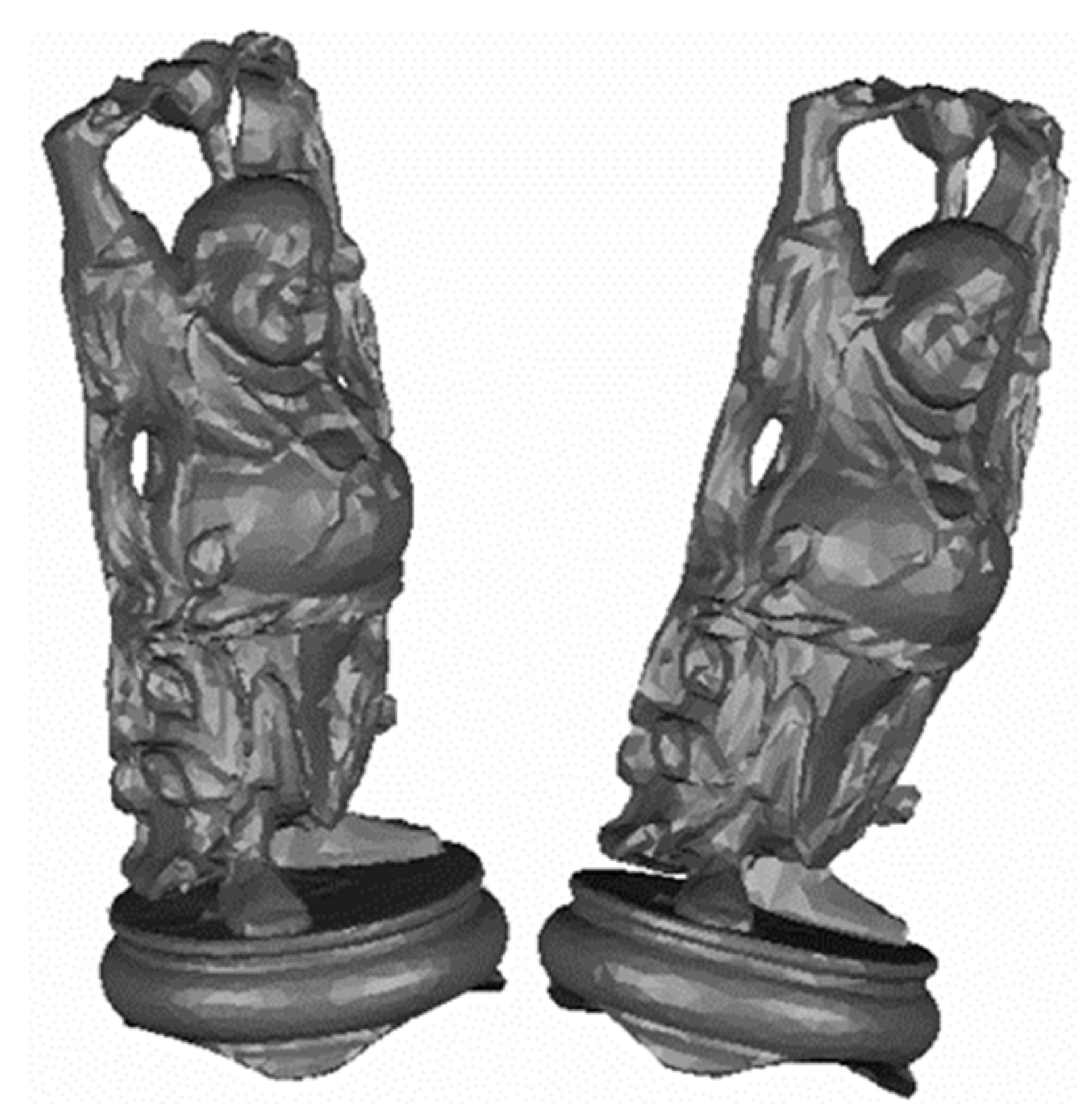
3.1. The Simulation Expriments Datasets

In simulation experiment 1, every point set was rotated 10, 20, 20 degrees and translated 0.05, 0.1, 0.1 m in x-, y- and z-directions, respectively. For the most practical applications where the point cloud was not 100% overlap, we also matched the several point clouds with partial overlap.

In simulation experiment 2, we used Happy Buddha point clouds from the Bologna dataset. This dataset is generated by randomly rotating and translating three to five models, which are from the Stanford 3D scanning warehouse, to create clutter variances. The Happy Buddha point clouds from different sample scenes are shown in Figure 4.

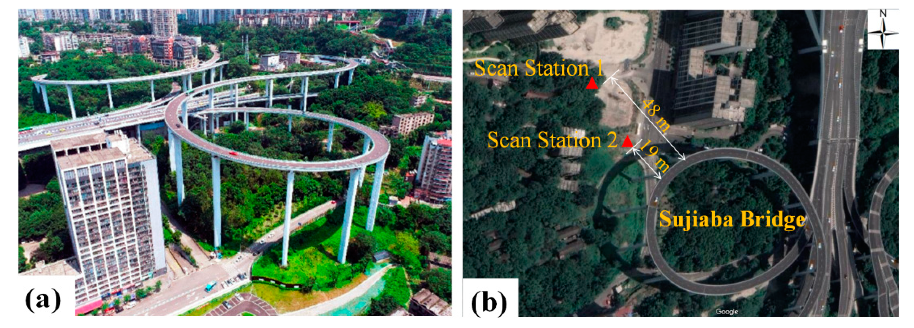
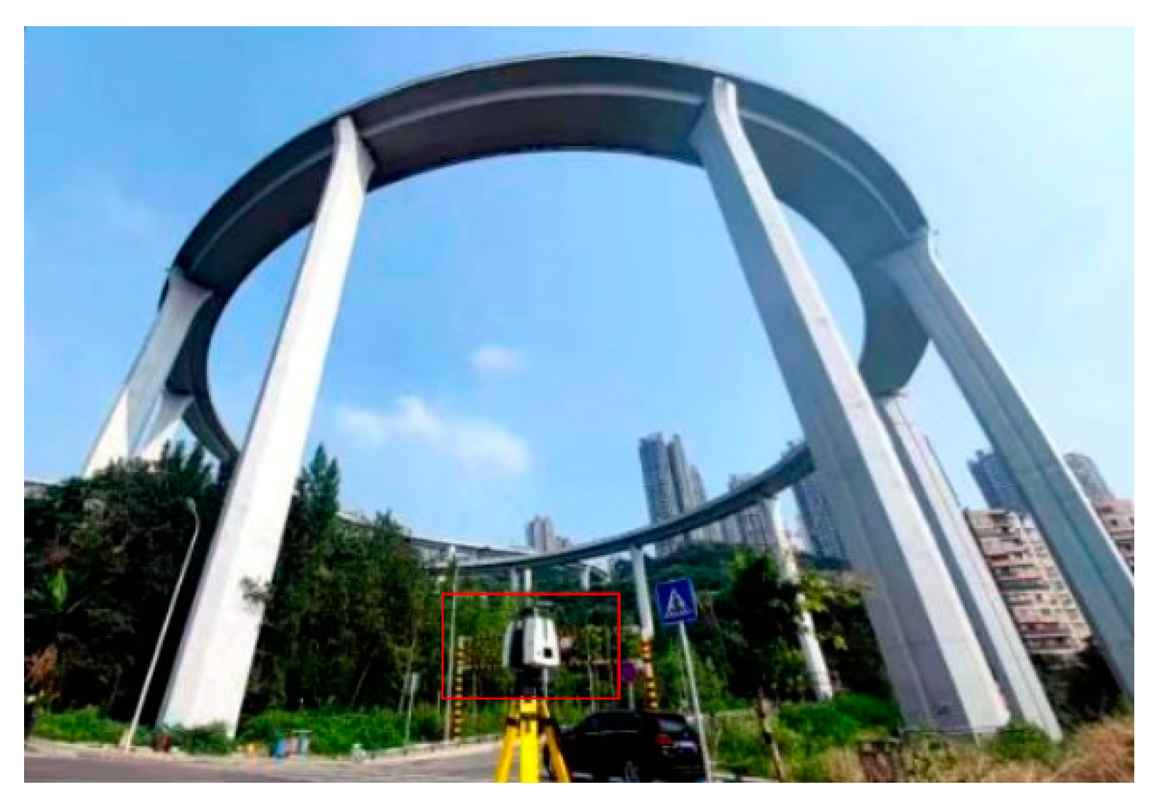
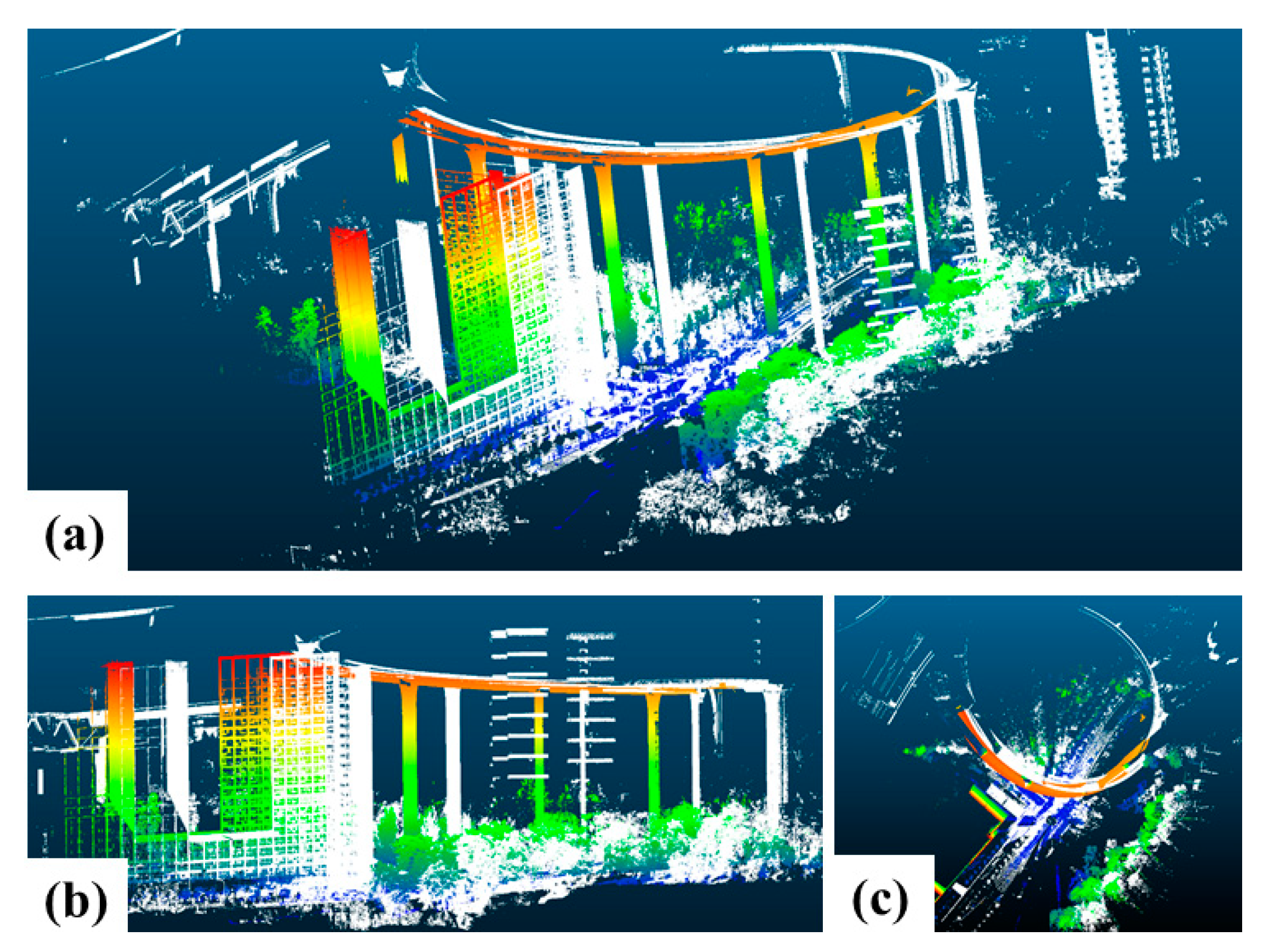
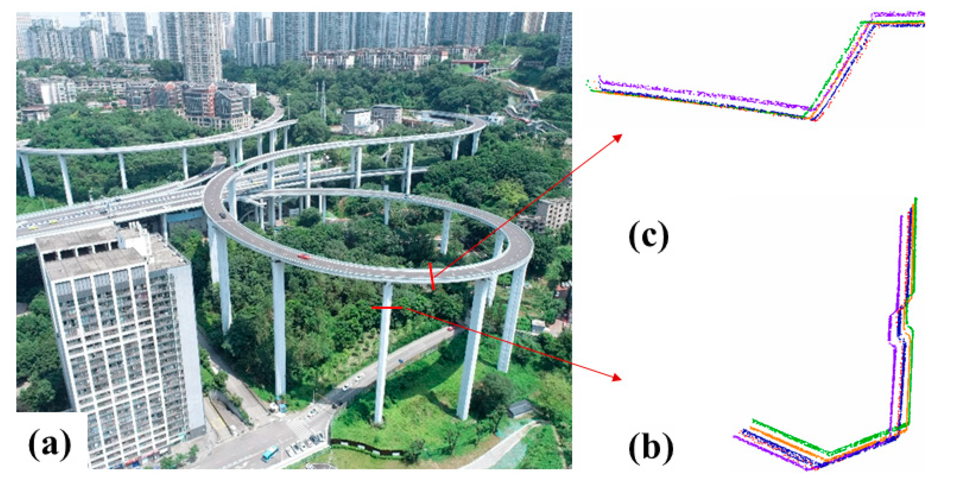
3.2. The Real Experiment Dataset

The real dataset was the TLS data of Sujiaba Bridge. The bridge is located in Nan’ an District, Chongqing, China. It is the highest ramp bridge in China, with the height of 72 m. In this study, we used a Leica P50 laser scanner to acquire data. The scanner is a ground-based 3D laser scanner that has the advantages of a long scanning range with minimal noise. The object studied, and photos showing Sujiaba Bridge are shown in Figure 5.

Table 1. Parameter of Leica P50 3D laser scanner [46].

Parameter	Value
Scan range mode	0.4~120 m, 0.4~270 m, 0.4~570 m, >1 km
Scan Rate	Maximum 1,000,000 points/s
Vertical/horizontal field-of-view	360°/290°
Range noise *	0.4 mm @ 10 m 0.5 mm @ 50 m
Dual-axis compensator	1.5″

* at 78% albedo.

lists the technical parameter of the Leica P50 laser scanner.

We collected TLS data of Sujiaba Bridge in two stations on 8 July 2021. The Sujiaba Bridge TLS data acquisition in scan station 1 is shown in Figure 6. The Leica P50 scanner was set near the bridge, the scanning range mode was set at 0.4~270 m, and the scanning resolution was set at 3 mm @ 10 m. The original point clouds of the bridge are shown in Figure 7.

4. Results and Discussions

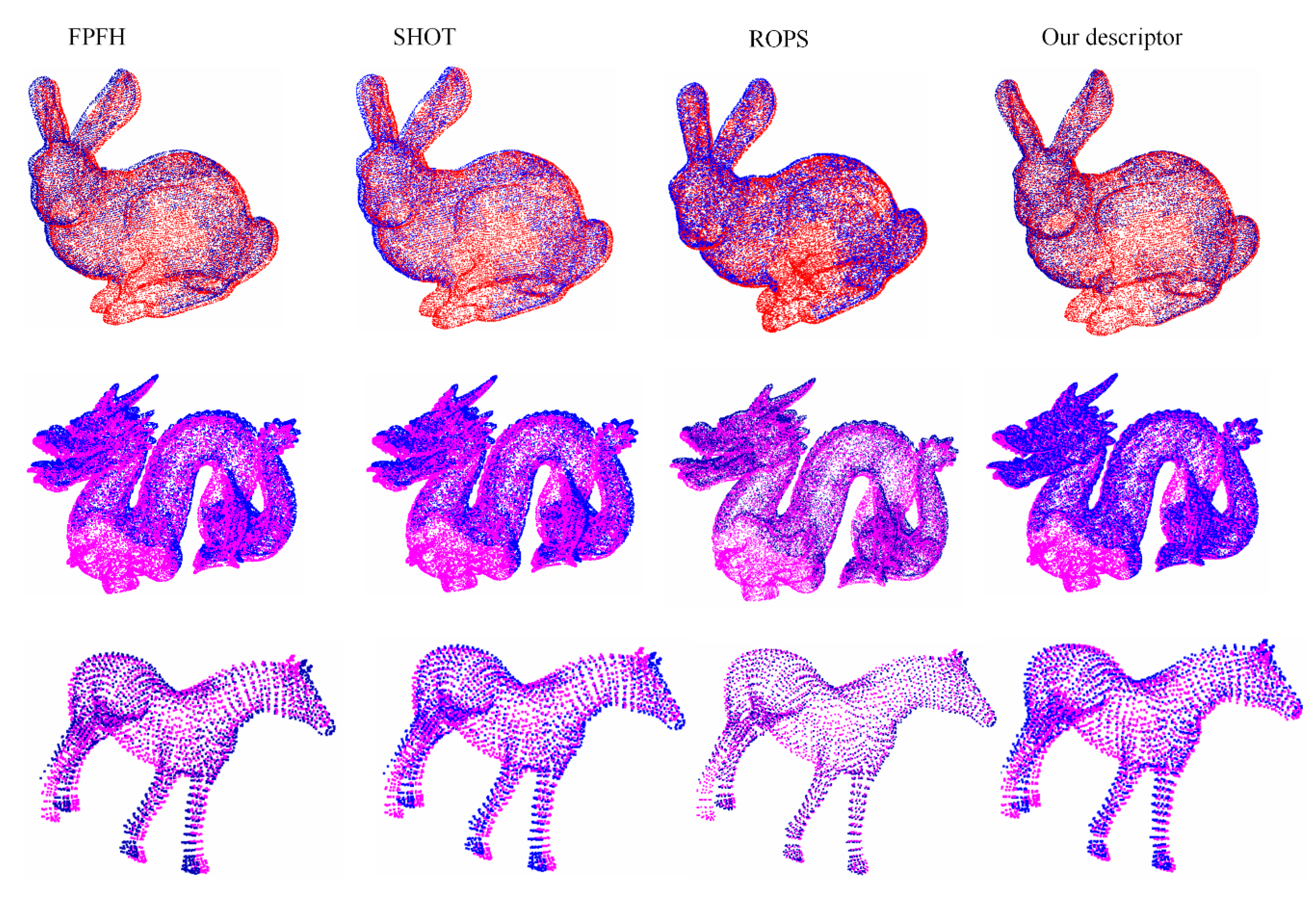
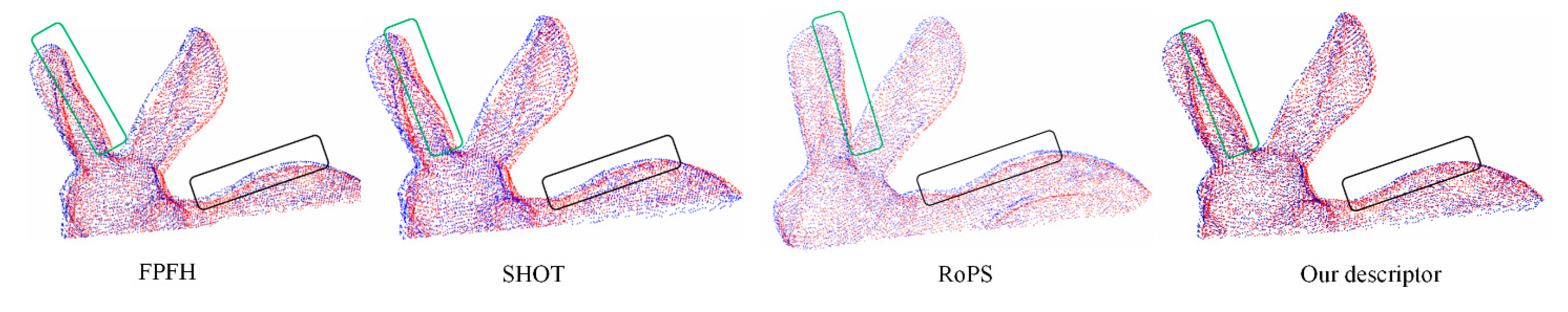
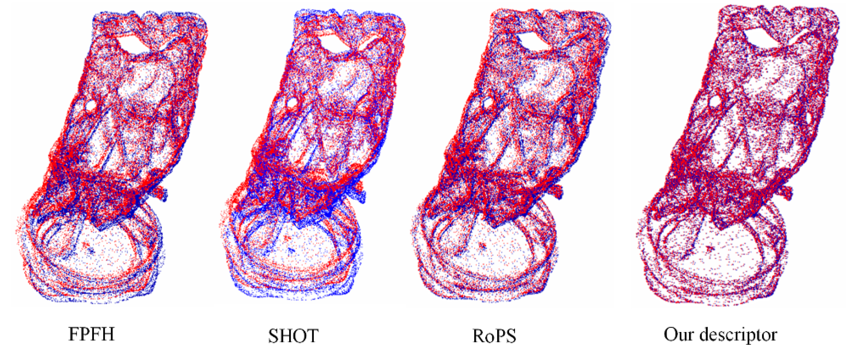
4.1. The Result of Simulation Experiments

The experimental result of point sets with an overlap percent of 0.6 is shown in Figure 8. It can be seen from Figure 8 that FPFH, SHOT, RoPS, and our descriptor all successfully register the datasets. The visual result of our descriptor has less distinctive patches of red or blue except for the non-overlap area. More explicitly, the enlarged registration result of the Bunny based on three descriptors is shown in Figure 9. The details of the ears and backs of the Bunny, based on our descriptor, achieve the best performance. Moreover, the details of other point clouds, such as the beards and tails of the Dragon, hooves, and mouth of the Horse, also visually show that the performance of our descriptor is better than FPFH, SHOT, and RoPS.

Table 2. Registration error with FPFH, SHOT, RoPS, and Our method on simulation experiment.

Dataset	Method	Rotation Error (°)			Translation Error (m)
		x	y	z	x	y	z
Bunny	FPFH	0.027	−0.018	0.034	−0.0032	0.0039	0.0028
	SHOT	0.021	−0.019	0.028	−0.0034	0.0025	0.0020
	RoPS	0.028	−0.017	0.023	−0.0029	0.0026	0.0024
	Our method	0.019	−0.013	0.021	−0.0019	0.0021	0.0017
Dragon	FPFH	−0.031	0.028	−0.043	0.0038	0.0026	−0.0036
	SHOT	−0.028	0.019	−0.036	0.0041	0.0024	−0.0029
	RoPS	−0.029	0.022	−0.038	0.0034	0.0025	−0.0031
	Our method	−0.023	0.014	−0.021	0.0032	0.0018	−0.0029
Horse	FPFH	−0.026	−0.025	0.023	0.0021	−0.0033	−0.0031
	SHOT	−0.023	−0.026	0.031	0.0025	−0.0036	−0.0029
	RoPS	−0.024	−0.023	0.027	0.0023	−0.0028	−0.0026
	Our method	−0.014	−0.016	0.017	0.0018	−0.0029	−0.0024

lists the rotation and translation errors along the x-, y-, and z-directions by using three different methods. It can be seen from Table 2 that the registration error of our method on three-point sets is very small. It further demonstrates the effectiveness of our algorithm. If a fine PCR is conducted, especially the commonly applied ICP algorithm, our algorithm provides a good initial pose. It will speed the ICP iterative convergence by only fewer iterations. Note that our method significantly outperforms than FPFH, SHOT, and RoPS methods.

The registration result of the Happy Buddha based on FPFH, SHOT, RoPS, and our proposed method is shown in Figure 10. The FPFH, SHOT, RoPS, and our descriptor also successfully register the real datasets. The visual result of our descriptor has less distinctive patches of red or blue. The details of the Happy Buddha edge also visually show the performance of our descriptor is better than FPFH, SHOT, and RoPS.

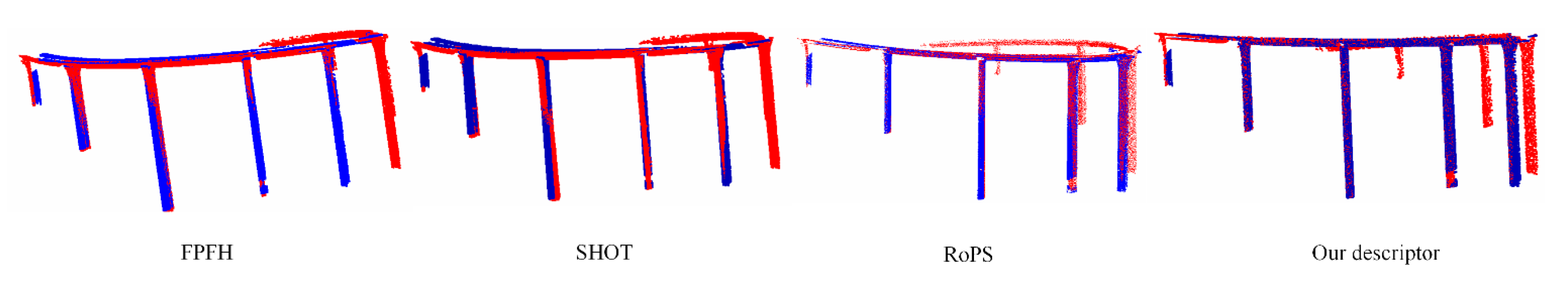
4.2. The Result of Real Experiment

The PCR result of FPFH, SHOT, RoPS, and our proposed method on Sujiaba TLS data is shown in Figure 11. It can be seen from Figure 11 that FPFH, SHOT, RoPS, and our descriptor also successfully register the real datasets. Moreover, our descriptor also has less distinctive patches of red or blue except for the non-overlap area. The comparison of the detailed registration result of Sujiaba Bridge based on four methods is shown in Figure 12. From the enlarged details of specified cross-section in bridge piers with top view and in main girders with side view, we clearly see that the distance between registration result based on our descriptor (blue) and the target point cloud (red) is the closet. It shows that our descriptor has the smallest translation error corresponding to the target point cloud. In addition, the purple line (FPFH), orange line (SHOT), and green line (RoPS) intersect with the blue line (target) at a large angle. It demonstrates that the result of FPFH, SHOT, and RoPS have a bigger rotation angle error than our descriptor. It further demonstrates that our descriptor significantly outperforms FPFH, SHOT, and RoPS methods in the real scan dataset.

The time consumption of our descriptor is obtained with similar accuracy. However, it should be noted that the time of our descriptor is the smallest. It is mainly because the method proposed has a low calculation dimension. The dimension of our descriptor is 32. Meanwhile, the FPFH is 33, the SHOT is 352, and the RoPS is 135. Although FPFH has only 33 dimensions, the extraction time is high because SPFH is calculated twice [47].

In general, the FPFH, SHOT, RoPS, and our proposed method successfully register the synthetic and real datasets. The PCR error of our method is the smallest. Additionally, the PCR speed of the method proposed herein is the fastest. The proposed method aims to establish a fast descriptor for PCR. After the experiment on the simulation and real datasets, the advantages of our method are summarized as follows.

(1)

In terms of precision, our method achieves a better performance than FPFH, SHOT, and RoPS. The wrong matching correspondences will occur because of high self-similar features. The classic algorithm RANSAC is mostly used for rejecting mismatches [48,49]. However, the RANSAC struggles to identify the mismatches. Therefore, it still has room for improvement in terms of precision. We selected the typical feature of the point cloud, which is invariant for transformation. Then we integrated the sub-feature into a new comprehensive descriptor. More importantly, we used the OSAC algorithm to eliminate wrong matching correspondences. The test results show that the new descriptor proposed herein has high precision and low dimension. In addition, our method does not rely on the good initial pose of the point cloud. It is practical for real data with unknown orientation.

(2)

In terms of consuming time, the well-known descriptors, such as FPFH, SHOT, and RoPS, occupy a large amount of data memory [50,51,52]. Meanwhile, most processes in our method are based on 3D key points. Besides the original point cloud, only the 32D descriptor are stored in the memory. Moreover, FPFH, SHOT, and RoPS have lower matching efficiency because of their feature dimensions [53]. Due to the low memory footprint and high PCR speed, our method has significant advantages.

The proposed method also has some limitations; we used an empirical equation to integrate the four sub-features. It is simple, easy to implement and strict in theory. However, it is not compact and may cause redundancy. In particular, to meet the requirements of bridge health monitoring, the quality of the bridge point cloud should be very high. The characteristics of the bridge point cloud are very particular. For example, the x-o-y plane of bridge TLS data should be an absolute horizontal plane. The dual-axis compensator of the Leica P50 scanner can achieve an accuracy of 1.5″ [11]. We try to decorrelate the values based on the characteristics of the bridge point cloud in the future. The sub-feature fusion algorithm should be further studied to obtain a more reasonable descriptor.

5. Conclusions

In this paper, we proposed a PCR method based on a novel local feature descriptor for point clouds. First, a new feature descriptor was designed by combining normal information, dot product, neighborhood distance, and curvature. Second, we established point-to-point correspondences based on feature descriptors via the popular distance metric L2 norm and apply the OSAC algorithm to eliminate false matching correspondences. Finally, we performed experiments on simulation and real datasets. We compared the performance of our proposed descriptor with well-known methods FPFH, SHOT, and RoPS.

In the first experiment, FPFH, SHOT, RoPS, and our descriptor all successfully register several synthetic datasets. The result of simulation experiments shows that the rotation angle error is below 0.025°, and the translation distance error is below 0.0035 m. Our method achieves an encouraging result, especially in detail. The real data test shows that the PCR errors based on our descriptor are smaller than FPFH, SHOT, and RoPS methods. Compared with the existing popular method, our proposed algorithm maintains a similar accuracy level with higher efficiency.

In general, considering the complexity of feature description and the high demands on calculating resources in practical applications, our method maintains a high registration accuracy with fast speed and low memory footprint. It is more suitable for practical TLS data.

References

1. Remondino, F. From point cloud to surface: The modeling and visualization problem. In Proceedings of the ISPRS WG V/6 Workshop “Visualization and Animation of Reality-Based 3D Models”, Tarasp-Vulpera, Switzerland, 24–28 February 2003; International Archives of the Photogrammetry, Remote Sensing and Spatial Information Sciences. p. 34. [Google Scholar]
2. Sahebdivani, S.; Arefi, H.; Maboudi, M. Rail track detection and projection-based 3D modeling from UAV point cloud. Sensors 2020, 20, 5220. [Google Scholar] [CrossRef]
3. Wang, X.; Mizukami, Y.; Tada, M.; Matsuno, F. Navigation of a mobile robot in a dynamic environment using a point cloud map. Artif. Life Robot. 2021, 26, 10–20. [Google Scholar] [CrossRef]
4. Rosas-Cervantes, V.; Lee, S.G. 3D localization of a mobile robot by using Monte Carlo algorithm and 2D features of 3D point cloud. Int. J. Control Autom. Syst. 2020, 18, 2955–2965. [Google Scholar] [CrossRef]
5. Perez-Grau, F.J.; Caballero, F.; Viguria, A.; Ollero, A. Multi-sensor three-dimensional Monte Carlo localization for long-term aerial robot navigation. Int. J. Adv. Robot. Syst. 2017, 14, 1729881417732757. [Google Scholar] [CrossRef]
6. Alhamzi, K.; Elmogy, M.; Barakat, S. 3D object recognition based on local and global features using point cloud library. Int. J. Adv. Comput. Technol. 2015, 7, 43. [Google Scholar]
7. Pratama, A.R.P.; Dewantara, B.S.B.; Sari, D.M.; Pramadihanto, D. Density-based Clustering for 3D Stacked Pipe Object Recognition using Directly-given Point Cloud Data on Convolutional Neural Network. EMITTER Int. J. Eng. Technol. 2022, 10, 153–169. [Google Scholar]
8. Bai, X.; Hu, Z.; Zhu, X.; Huang, Q.; Chen, Y.; Fu, H.; Tai, C. Transfusion: Robust lidar-camera fusion for 3D object detection with transformers. In Proceedings of the IEEE/CVF Conference on Computer Vision and Pattern Recognition, New Orleans, LA, USA, 21–24 June 2022; pp. 1090–1099. [Google Scholar]
9. Mineo, C.; Pierce, S.G.; Summan, R. Novel algorithms for 3D surface point cloud boundary detection and edge reconstruction. J. Comput. Des. Eng. 2019, 6, 81–91. [Google Scholar] [CrossRef]
10. Sun, T.; Liu, G.; Li, R.; Liu, S.; Zhu, S.; Zeng, B. Quadratic terms based point-to-surface 3D representation for deep learning of point cloud. IEEE Trans. Circuits Syst. Video Technol. 2021, 32, 2705–2718. [Google Scholar] [CrossRef]
11. Zhou, Y.; Han, D.; Hu, K.; Qin, G.; Xiang, Z.; Ying, C.; Zhao, L.; Hu, X. Accurate virtual trial assembly method of prefabricated steel components using terrestrial laser scanning. Adv. Civ. Eng. 2021, 2021, 9916859. [Google Scholar] [CrossRef]
12. Zhao, L.; Ma, X.; Xiang, Z.; Zhang, S.; Hu, C.; Zhou, Y.; Chen, G. Landslide Deformation Extraction from Terrestrial Laser Scanning Data with Weighted Least Squares Regularization Iteration Solution. Remote Sens. 2022, 14, 2897. [Google Scholar] [CrossRef]
13. Sharp, G.C.; Lee, S.W.; Wehe, D.K. ICP registration using invariant features. IEEE Trans. Pattern Anal. Mach. Intell. 2002, 24, 90–102. [Google Scholar] [CrossRef]
14. Maken, F.A.; Ramos, F.; Ott, L. Stein ICP for Uncertainty Estimation in Point Cloud Matching. IEEE Robot. Autom. Lett. 2021, 7, 1063–1070. [Google Scholar] [CrossRef]
15. Cheng, L.; Chen, S.; Liu, X.; Xu, H.; Wu, Y.; Li, M.; Chen, Y. Registration of laser scanning point clouds: A review. Sensors 2018, 18, 1641. [Google Scholar] [CrossRef] [PubMed]
16. Huang, X.; Zhang, J.; Wu, Q.; Fan, L. A coarse-to-fine algorithm for matching and registration in 3D cross-source point clouds. IEEE Trans. Circuits Syst. Video Technol. 2017, 28, 2965–2977. [Google Scholar] [CrossRef]
17. Yu, H.; Li, F.; Saleh, M.; Busam, B.; Ilic, S. Cofinet: Reliable coarse-to-fine correspondences for robust pointcloud registration. Adv. Neural Inf. Process. Syst. 2021, 34, 23872–23884. [Google Scholar]
18. Xie, Z.; Xu, S.; Li, X. A high-accuracy method for fine registration of overlapping point clouds. Image Vis. Comput. 2010, 28, 563–570. [Google Scholar] [CrossRef]
19. Jaw, J.; Chuang, T. Feature-based registration of terrestrial lidar point clouds. Int. Arch. Photogramm. Remote Sens. Spat. Inf. Sci. 2008, 37, 2. [Google Scholar]
20. Xia, T.; Yang, J.; Chen, L. Automated semantic segmentation of bridge point cloud based on local descriptor and machine learning. Autom. Constr. 2022, 133, 103992. [Google Scholar] [CrossRef]
21. Belongie, S.; Malik, J.; Puzicha, J. Shape matching and object recognition using shape contexts. IEEE Trans. Pattern Anal. Mach. Intell. 2002, 24, 509–522. [Google Scholar] [CrossRef]
22. Makadia, A.; Patterson, A.; Daniilidis, K. Fully automatic registration of 3D point clouds. In Proceedings of the 2006 IEEE Computer Society Conference on Computer Vision and Pattern Recognition (CVPR’06), New York, NY, USA, 17–22 June 2006; Volume 1, pp. 1297–1304. [Google Scholar]
23. Dold, C. Extended Gaussian images for the registration of terrestrial scan data. In Proceedings of the ISPRS Workshop Laser Scanning, Enschede, The Netherlands, 12–14 September 2005; pp. 180–185. [Google Scholar]
24. Poiesi, F.; Boscaini, D. Generalisable and distinctive 3D local deep descriptors for point cloud registration. arXiv 2022, arXiv:2105.10382. [Google Scholar]
25. Bai, X.; Luo, Z.; Zhou, L.; Fu, H.; Quan, L.; Tai, C. D3feat: Joint learning of dense detection and description of 3D local features. In Proceedings of the IEEE/CVF Conference on Computer Vision and Pattern Recognition, Seattle, WA, USA, 13–19 June 2020; pp. 6359–6367. [Google Scholar]
26. Petricek, T.; Svoboda, T. Point cloud registration from local feature correspondences—Evaluation on challenging datasets. PLoS ONE 2017, 12, e0187943. [Google Scholar] [CrossRef] [PubMed]
27. Huang, X.; Mei, G.; Zhang, J.; Abbas, R. A comprehensive survey on point cloud registration. arXiv 2021, arXiv:2103.02690. [Google Scholar]
28. Kiforenko, L.; Drost, B.; Tombari, F.; Krüger, N.; Buch, A.G. A performance evaluation of point pair features. Comput. Vis. Image Underst. 2018, 166, 66–80. [Google Scholar] [CrossRef]
29. Johnson, A.E.; Hebert, M. Using spin images for efficient object recognition in cluttered 3D scenes. IEEE Trans. Pattern Anal. Mach. Intell. 1999, 21, 433–449. [Google Scholar] [CrossRef]
30. Buch, A.G.; Kraft, D.; Robotics, S. Local Point Pair Feature Histogram for Accurate 3D Matching. In Proceedings of the BMVC, Newcastle, UK, 3–6 September 2018; p. 143. [Google Scholar]
31. Rusu, R.B.; Blodow, N.; Beetz, M. Fast point feature histograms (FPFH) for 3D registration. In Proceedings of the 2009 IEEE International Conference on Robotics and Automation, Kobe, Japan, 12–17 May 2009; pp. 3212–3217. [Google Scholar]
32. Tombari, F.; Salti, S.; Stefano, L.D. Unique signatures of histograms for local surface description. In Proceedings of the European Conference on Computer Vision, Heraklion, Greece, 5–11 September 2010; Springer: Berlin/Heidelberg, Germany, 2010; pp. 356–369. [Google Scholar]
33. Salti, S.; Tombari, F.; Stefano, L.D. SHOT: Unique signatures of histograms for surface and texture description. Comput. Vis. Image Underst. 2014, 125, 251–264. [Google Scholar] [CrossRef]
34. Guo, Y.; Sohel, F.; Bennamoun, M.; Lu, M.; Wan, J. Rotational projection statistics for 3D local surface description and object recognition. Int. J. Comput. Vis. 2013, 105, 63–86. [Google Scholar] [CrossRef] [Green Version]
35. Yang, J.; Zhang, Q.; Xiao, Y.; Cao, Z. TOLDI: An effective and robust approach for 3D local shape description. Pattern Recognit. 2017, 65, 175–187. [Google Scholar] [CrossRef]
36. Bai, X.; Luo, Z.; Zhou, L.; Chen, H.; Li, L.; Hu, Z.; Fu, H.; Tai, C. Pointdsc: Robust point cloud registration using deep spatial consistency. In Proceedings of the IEEE/CVF Conference on Computer Vision and Pattern Recognition, Nashville, TN, USA, 20–25 June 2021; pp. 15859–15869. [Google Scholar]
37. Vosselman, G.; Gorte, B.G.H.; Sithole, G.; Rabbani, T. Recognising structure in laser scanner point clouds. Int. Arch. Photogramm. Remote Sens. Spat. Inf. Sci. 2004, 46, 33–38. [Google Scholar]
38. Pauly, M.; Gross, M.; Kobbelt, L.P. Efficient simplification of point-sampled surfaces. In Proceedings of the IEEE Visualization 2002, VIS 2002, Boston, MA, USA, 27 October–1 November 2002; pp. 163–170. [Google Scholar]
39. Dong, Z.; Yang, B.; Liu, Y.; Liang, F.; Li, B.; Zang, Y. A novel binary shape context for 3D local surface description. ISPRS J. Photogramm. Remote Sens. 2017, 130, 431–452. [Google Scholar] [CrossRef]
40. Rusu, R.B.; Blodow, N.; Marton, Z.C.; Beetz, M. Aligning point cloud views using persistent feature histograms. In Proceedings of the 2008 IEEE/RSJ International Conference on Intelligent Robots and Systems, Nice, France, 22–26 September 2008; pp. 3384–3391. [Google Scholar]
41. Deakin, R.E. A Note on the Bursa-Wolf and Molodensky-Badekas Transformations; School of Mathematical and Geospatial Sciences, RMIT University: Melbourne, VIC, Australia, 2006; pp. 1–21. [Google Scholar]
42. Fischler, M.A.; Bolles, R.C. Random sample consensus: A paradigm for model fitting with applications to image analysis and automated cartography. Commun. ACM 1981, 24, 381–395. [Google Scholar] [CrossRef]
43. Yang, J.; Cao, Z.; Zhang, Q. A fast and robust local descriptor for 3D point cloud registration. Inf. Sci. 2016, 346, 163–179. [Google Scholar] [CrossRef]
44. The Standford 3D Scanning Repository. Available online: http://www-graphics.stanford.edu/data/3Dscanrep/ (accessed on 29 June 2022).
45. Available online: http://vision.deis.unibo.it/research/80-shot (accessed on 19 August 2022).
46. Leica ScanStation P50—Long Range 3D Terrestrial Laser Scanner. Available online: https://leica-geosystems.com/products/laser-scanners/scanners/leica-scanstation-p50 (accessed on 29 June 2022).
47. Deschaud, J.E.; Goulette, F. Point cloud non local denoising using local surface descriptor similarity. IAPRS 2010, 38, 109–114. [Google Scholar]
48. Liu, L.; Xiao, J.; Wang, Y.; Lu, Z.; Wang, Y. A novel rock-mass point cloud registration method based on feature line extraction and feature point matching. IEEE Trans. Geosci. Remote Sens. 2021, 60, 5701117. [Google Scholar] [CrossRef]
49. Prakhya, S.M.; Lin, J.; Chandrasekhar, V.; Lin, W.; Liu, B. 3DHoPD: A fast low-dimensional 3-D descriptor. IEEE Robot. Autom. Lett. 2017, 2, 1472–1479. [Google Scholar] [CrossRef]
50. Lei, H.; Jiang, G.; Quan, L. Fast descriptors and correspondence propagation for robust global point cloud registration. IEEE Trans. Image Process. 2017, 26, 3614–3623. [Google Scholar] [CrossRef]
51. Dong, T.; Zhao, Y.; Zhang, Q.; Xue, B.; Li, J.; Li, W. Multi-scale point cloud registration based on topological structure. Concurr. Comput. Pract. Exp. 2022, e6873. [Google Scholar] [CrossRef]
52. Lu, J.; Wang, Z.; Hua, B.; Chen, K. Automatic point cloud registration algorithm based on the feature histogram of local surface. PLoS ONE 2020, 15, e0238802. [Google Scholar] [CrossRef]
53. He, Y.; Yang, J.; Hou, X.; Pang, S.; Chen, J. ICP registration with DCA descriptor for 3D point clouds. Opt. Express 2021, 29, 20423–20439. [Google Scholar] [CrossRef]
Figure 1. The schematic of the proposed descriptor. (a) The original point cloud. (b) Keypoints. (c) The enlarged detail of the red circle and its surrounding points in (b) image. (d) The neighboring points of a specified point. (e) Feature descriptor.
Remotesensing 14 04346 g001
Figure 2. The diagram of sub-feature f 1 and f 2 .
Remotesensing 14 04346 g002
Figure 3. The diagram of distance parameter f 3 . pi is the key point, r is the radius neighborhood of the key point, p k i is the point in the neighborhood sphere with the radius r.
Remotesensing 14 04346 g003
Figure 4. The Happy Buddha point cloud. Note that the point clouds are in ply format.
Remotesensing 14 04346 g004
Figure 5. Photos showing Sujiaba Bridge. (a) UAV image of Sujiaba Bridge; (b) the schematic diagram of scan station in Sujiaba Bridge and the background is from Google Maps. The scan station 1 is 48 m away from the bridge and station 2 is 19 m away from the bridge.
Remotesensing 14 04346 g005
Figure 6. Sujiaba Bridge TLS data acquisition in scan station 1. The red box shows the Leica P50 3D laser scanner.
Remotesensing 14 04346 g006
Figure 7. The original point cloud of Sujiaba Bridge. (a) free view. (b) side view. (c) top view. The TLS data of station 1 is shown in white. The colorful points are the TLS data of station 2. The two-point sets with partial overlap.
Remotesensing 14 04346 g007
Figure 8. Comparison PCR results based on four descriptors, and the overlap ratio is 0.6. The overlap is measured with respect to the surface area. From left to right is the result of FPFH, SHOT, RoPS, and our descriptor, respectively. From top to down is the Bunny, Dragon, and Horse point cloud, respectively. The source point cloud is shown in blue, and the target point cloud is shown in red.
Remotesensing 14 04346 g008
Figure 9. Enlarged result of Bunny based on four descriptors. From left to right is the result of FPFH, SHOT, RoPS, and our descriptor, respectively. The source point cloud is shown in blue, and the target point cloud is shown in red. The black box shows details of the rabbit’s back with a sharp edge, and the green box shows details of the rabbit’s ears.
Remotesensing 14 04346 g009
Figure 10. Comparison Happy Buddha registration result based on four descriptors. From left to right is the result of FPFH, SHOT, RoPS and our descriptor respectively. The source point cloud is shown in blue, and the target point cloud is shown in red.
Remotesensing 14 04346 g010
Figure 11. PCR result of Sujiaba Bridge based on four methods. From left to right is the result of FPFH, SHOT, RoPS, and our descriptors, respectively. The source point cloud is shown in blue, and the target point cloud is shown in red.
Remotesensing 14 04346 g011
Figure 12. Comparison of enlarged registration results of Sujiaba Bridge based on four methods. (a) UAV image of Sujiaba Bridge. (b) Enlarged details of specified cross-section in bridge piers with top view. (c) Enlarged details of specified cross-section in main girders with side view. The target point cloud is shown in red. The result of FPFH, SHOT, RoPS, and our descriptor is shown in purple, orange, green, and blue, respectively.
Remotesensing 14 04346 g012