
3D Reconstruction of Remote Sensing Mountain Areas with TSDF-Based Neural Networks

Abstract
:
1. Introduction
- We investigate the problem of outdoor 3D mountain reconstruction and propose a new TSDF-based reconstruction method. A challenging synthetic dataset is built for this problem.
- We propose a feature enhancement (FE) module, view fusion via reweighted mechanism (VRM), and a spatial–temporal aggregation (STA) module to effectively utilize features from different 2D views and improve feature discriminative capability on voxels. With the above design, we outperform other state-of-the-art TSDF-based methods on our task.
2. Background and Related Work
2.1. Truncated Signed Distance Function (TSDF)
2.2. Depth Estimation
2.3. TSDF-Based Reconstruction
2.4. Implicit Neural Representation
3. Materials and Methods
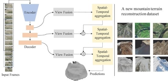
3.1. Overview
3.2. Feature Enhancement Module
3.3. View Fusion via Reweighted Mechanisms
3.4. Spatial-Temporal Aggregation Module
3.5. Implementation Details
4. Results
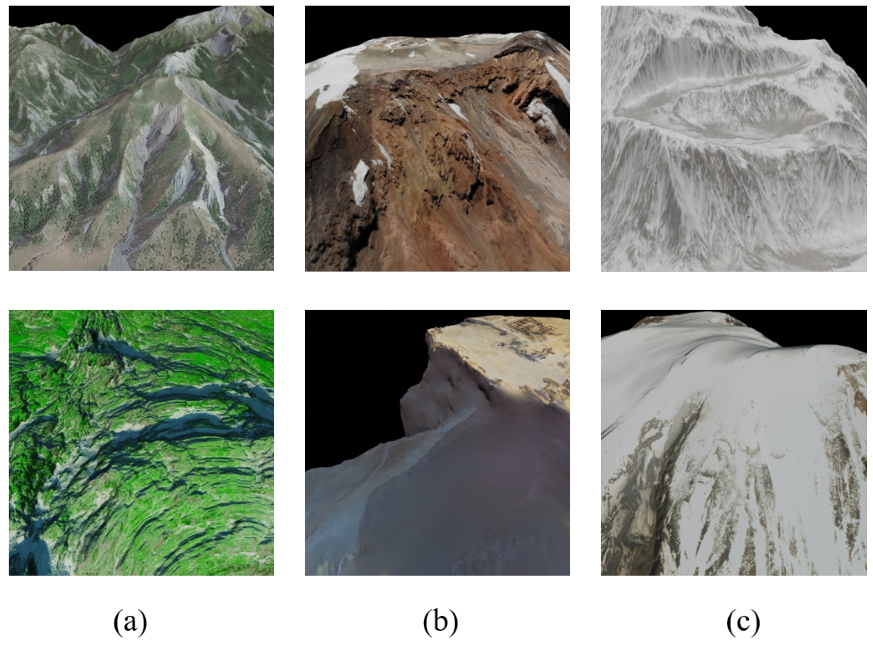
4.1. Dataset
4.2. Comparison Methods and Metrics
4.3. Overall Comparison on the Synthetic Dataset
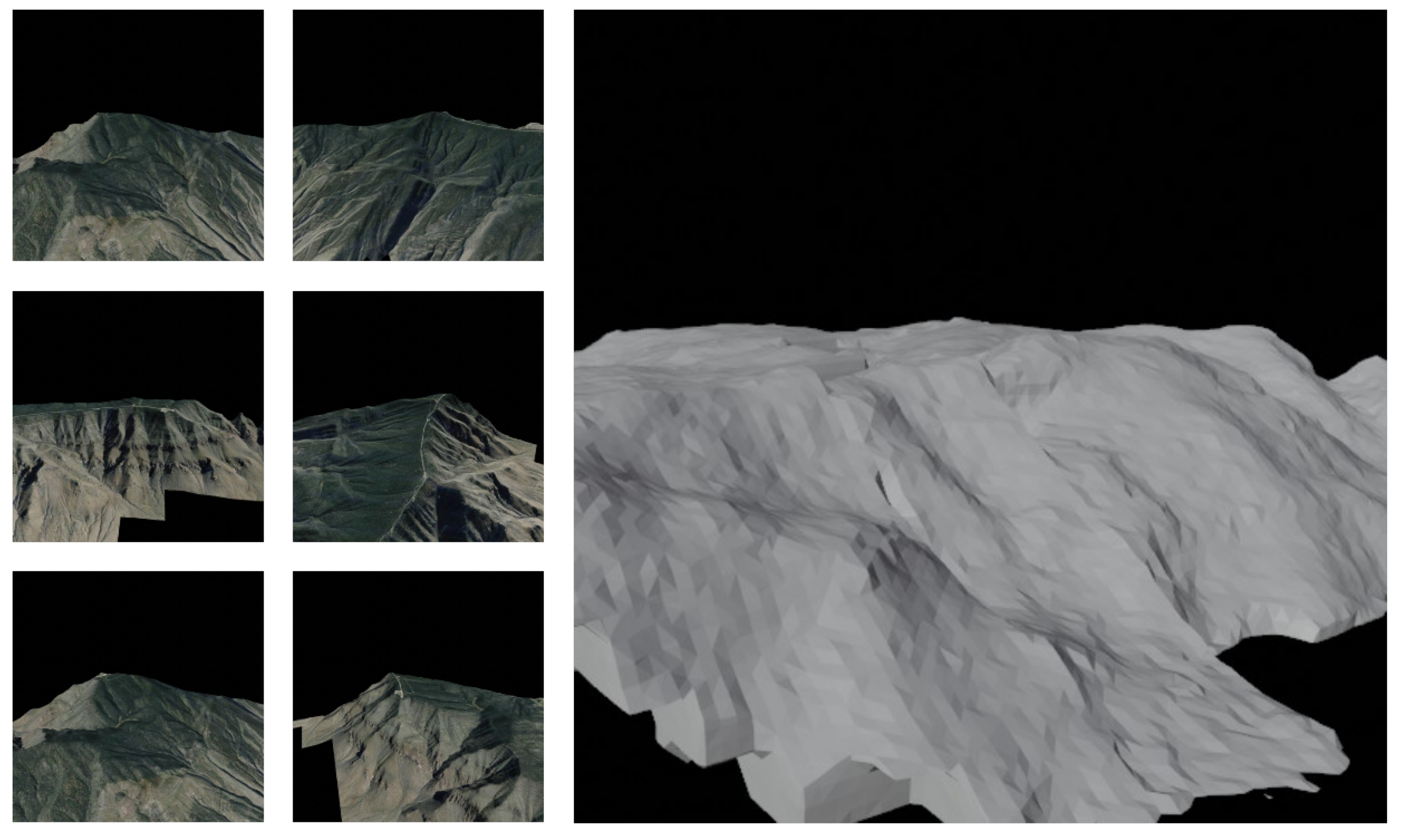
4.4. Generalizing to Real Data
5. Discussion
5.1. Ablation Study
5.2. Limitations and Future
6. Conclusions
Author Contributions
Funding
Data Availability Statement
Acknowledgments
Conflicts of Interest
References
- Li, H.; Chen, S.; Wang, Z.; Li, W. Fusion of LiDAR data and orthoimage for automatic building reconstruction. In Proceedings of the IEEE International Geoscience and Remote Sensing Symposium, IGARSS 2010, Honolulu, HI, USA, 25–30 July 2010. [Google Scholar]
- Xiong, B.; Jiang, W.; Li, D.; Qi, M. Voxel Grid-Based Fast Registration of Terrestrial Point Cloud. Remote Sens. 2021, 13, 1905. [Google Scholar] [CrossRef]
- Schiavulli, D.; Nunziata, F.; Migliaccio, M.; Frappart, F.; Ramilien, G.; Darrozes, J. Reconstruction of the Radar Image From Actual DDMs Collected by TechDemoSat-1 GNSS-R Mission. IEEE J. Sel. Top. Appl. Earth Obs. Remote Sens. 2016, 9, 4700–4708. [Google Scholar] [CrossRef]
- Aghababaee, H.; Ferraioli, G.; Schirinzi, G.; Pascazio, V. Corrections to “Regularization of SAR Tomography for 3-D Height Reconstruction in Urban Areas” [Feb 19 648–659]. Sel. Top. Appl. Earth Obs. Remote Sens. IEEE J. 2019, 12, 1063. [Google Scholar] [CrossRef]
- Wang, M.; Wei, S.; Shi, J.; Wu, Y.; Tian, B. CSR-Net: A Novel Complex-valued Network for Fast and Precise 3-D Microwave Sparse Reconstruction. IEEE J. Sel. Top. Appl. Earth Obs. Remote Sens. 2020, 13, 4476–4492. [Google Scholar] [CrossRef]
- Yang, Y.C.; Lu, C.Y.; Huang, S.J.; Yang, T.Z.; Chang, Y.C.; Ho, C.R. On the Reconstruction of Missing Sea Surface Temperature Data from Himawari-8 in Adjacent Waters of Taiwan Using DINEOF Conducted with 25-h Data. Remote Sens. 2022, 14, 2818. [Google Scholar] [CrossRef]
- Zhang, E.; Fu, Y.; Wang, J.; Liu, L.; Yu, K.; Peng, J. MSAC-Net: 3D Multi-Scale Attention Convolutional Network for Multi-Spectral Imagery Pansharpening. Remote Sens. 2022, 14, 2761. [Google Scholar] [CrossRef]
- Williams, S.; Parker, L.T.; Howard, A.M. Terrain Reconstruction of Glacial Surfaces: Robotic Surveying Techniques. Robot. Autom. Mag. IEEE 2012, 19, 59–71. [Google Scholar] [CrossRef]
- Kazhdan, M.; Bolitho, M.; Hoppe, H. Poisson surface reconstruction. In Proceedings of the Fourth Eurographics Symposium on Geometry Processing, Cagliari Sardinia, Italy, 26–28 June 2006; Volume 7. [Google Scholar]
- Lorensen, W.E.; Cline, H.E. Marching cubes: A high resolution 3D surface construction algorithm. ACM Siggraph Comput. Graph. 1987, 21, 163–169. [Google Scholar] [CrossRef]
- Murez, Z.; van As, T.; Bartolozzi, J.; Sinha, A.; Badrinarayanan, V.; Rabinovich, A. Atlas: End-to-end 3d scene reconstruction from posed images. In Proceedings of the Computer Vision–ECCV 2020: 16th European Conference, Glasgow, UK, 23–28 August 2020; Part VII 16. Springer: Berlin/Heidelberg, Germany, 2020; pp. 414–431. [Google Scholar]
- Choe, J.; Im, S.; Rameau, F.; Kang, M.; Kweon, I.S. Volumefusion: Deep depth fusion for 3d scene reconstruction. In Proceedings of the IEEE/CVF International Conference on Computer Vision, Montreal, QC, Canada, 11 October 2021; pp. 16086–16095. [Google Scholar]
- Sun, J.; Xie, Y.; Chen, L.; Zhou, X.; Bao, H. NeuralRecon: Real-Time Coherent 3D Reconstruction from Monocular Video. In Proceedings of the IEEE/CVF Conference on Computer Vision and Pattern Recognition, Nashville, TN, USA, 20–25 June 2021; pp. 15598–15607. [Google Scholar]
- Bozic, A.; Palafox, P.; Thies, J.; Dai, A.; Nießner, M. Transformerfusion: Monocular rgb scene reconstruction using transformers. Adv. Neural Inf. Process. Syst. 2021, 34, 1403–1414. [Google Scholar]
- Chang, A.X.; Funkhouser, T.; Guibas, L.; Hanrahan, P.; Huang, Q.; Li, Z.; Savarese, S.; Savva, M.; Song, S.; Su, H. ShapeNet: An Information-Rich 3D Model Repository. arXiv 2015, arXiv:1512.03012. [Google Scholar]
- Li, W.; Saeedi, S.; McCormac, J.; Clark, R.; Tzoumanikas, D.; Ye, Q.; Huang, Y.; Tang, R.; Leutenegger, S. Interiornet: Mega-scale multi-sensor photo-realistic indoor scenes dataset. arXiv 2018, arXiv:1809.00716. [Google Scholar]
- Grinvald, M.; Tombari, F.; Siegwart, R.; Nieto, J. TSDF++: A Multi-Object Formulation for Dynamic Object Tracking and Reconstruction. In Proceedings of the 2021 IEEE International Conference on Robotics and Automation (ICRA), Xi’an, China, 30 May–5 June 2021. [Google Scholar]
- Kim, H.; Lee, B. Probabilistic TSDF Fusion Using Bayesian Deep Learning for Dense 3D Reconstruction with a Single RGB Camera. In Proceedings of the 2020 IEEE International Conference on Robotics and Automation (ICRA), Xi’an, China, 30 May–5 June 2020. [Google Scholar]
- Hardouin, G.; Morbidi, F.; Moras, J.; Marzat, J.; Mouaddib, E.M. Surface-driven Next-Best-View planning for exploration of large-scale 3D environments. IFAC-PapersOnLine 2020, 53, 15501–15507. [Google Scholar] [CrossRef]
- Yao, Y.; Luo, Z.; Li, S.; Fang, T.; Quan, L. Mvsnet: Depth inference for unstructured multi-view stereo. In Proceedings of the European Conference on Computer Vision (ECCV), Munich, Germany, 8–14 September 2018; pp. 767–783. [Google Scholar]
- Wang, F.; Galliani, S.; Vogel, C.; Speciale, P.; Pollefeys, M. PatchmatchNet: Learned Multi-View Patchmatch Stereo. In Proceedings of the IEEE/CVF Conference on Computer Vision and Pattern Recognition, Nashville, TN, USA, 20–25 June 2021; pp. 14194–14203. [Google Scholar]
- Vaswani, A.; Shazeer, N.; Parmar, N.; Uszkoreit, J.; Jones, L.; Gomez, A.N.; Kaiser, Ł.; Polosukhin, I. Attention is all you need. In Proceedings of the Advances in Neural Information Processing Systems, Long Beach, CA, USA, 4–9 December 2017; pp. 5998–6008.
- Newcombe, R.A.; Izadi, S.; Hilliges, O.; Molyneaux, D.; Kim, D.; Davison, A.J.; Kohi, P.; Shotton, J.; Hodges, S.; Fitzgibbon, A. Kinectfusion: Real-time dense surface mapping and tracking. In Proceedings of the 2011 10th IEEE International Symposium on Mixed and Augmented Reality, Basel, Switzerland, 26–29 October 2011; pp. 127–136. [Google Scholar]
- Im, S.; Jeon, H.G.; Lin, S.; Kweon, I.S. Dpsnet: End-to-end deep plane sweep stereo. arXiv 2019, arXiv:1905.00538. [Google Scholar]
- Hou, Y.; Kannala, J.; Solin, A. Multi-view stereo by temporal nonparametric fusion. In Proceedings of the IEEE/CVF International Conference on Computer Vision, Seoul, Korea, 27 October–2 November 2019; pp. 2651–2660. [Google Scholar]
- Wei, Y.; Liu, S.; Rao, Y.; Zhao, W.; Lu, J.; Zhou, J. Nerfingmvs: Guided optimization of neural radiance fields for indoor multi-view stereo. In Proceedings of the IEEE/CVF International Conference on Computer Vision, Montreal, QC, Canada, 11 October 2021; pp. 5610–5619. [Google Scholar]
- Kazhdan, M.; Hoppe, H. Screened poisson surface reconstruction. ACM Trans. Graph. (ToG) 2013, 32, 1–13. [Google Scholar] [CrossRef] [Green Version]
- Labatut, P.; Pons, J.P.; Keriven, R. Robust and efficient surface reconstruction from range data. In Computer Graphics Forum; Wiley Online Library: Hoboken, NJ, USA, 2009; Volume 28, pp. 2275–2290. [Google Scholar]
- Weder, S.; Schonberger, J.L.; Pollefeys, M.; Oswald, M.R. NeuralFusion: Online Depth Fusion in Latent Space. In Proceedings of the IEEE/CVF Conference on Computer Vision and Pattern Recognition, Nashville, TN, USA, 20–25 June 2021; pp. 3162–3172. [Google Scholar]
- Mildenhall, B.; Srinivasan, P.P.; Tancik, M.; Barron, J.T.; Ramamoorthi, R.; Ng, R. Nerf: Representing scenes as neural radiance fields for view synthesis. In Proceedings of the European Conference on Computer Vision, Glasgow, UK, 23–28 August 2020; Springer: Berlin/Heidelberg, Germany, 2020; pp. 405–421. [Google Scholar]
- Martin-Brualla, R.; Radwan, N.; Sajjadi, M.S.; Barron, J.T.; Dosovitskiy, A.; Duckworth, D. Nerf in the wild: Neural radiance fields for unconstrained photo collections. In Proceedings of the IEEE/CVF Conference on Computer Vision and Pattern Recognition, Nashville, TN, USA, 20–25 June 2021; pp. 7210–7219. [Google Scholar]
- Chen, Y.; Liu, S.; Wang, X. Learning continuous image representation with local implicit image function. In Proceedings of the IEEE/CVF Conference on Computer Vision and Pattern Recognition, Nashville, TN, USA, 20–25 June 2021; pp. 8628–8638. [Google Scholar]
- Xu, X.; Wang, Z.; Shi, H. UltraSR: Spatial Encoding is a Missing Key for Implicit Image Function-based Arbitrary-Scale Super-Resolution. arXiv 2021, arXiv:2103.12716. [Google Scholar]
- Skorokhodov, I.; Ignatyev, S.; Elhoseiny, M. Adversarial generation of continuous images. In Proceedings of the IEEE/CVF Conference on Computer Vision and Pattern Recognition, Nashville, TN, USA, 20–25 June 2021; pp. 10753–10764. [Google Scholar]
- Anokhin, I.; Demochkin, K.; Khakhulin, T.; Sterkin, G.; Korzhenkov, D. Image Generators with Conditionally-Independent Pixel Synthesis. In Proceedings of the IEEE/CVF Conference on Computer Vision and Pattern Recognition (CVPR), Nashville, TN, USA, 20–25 June 2021. [Google Scholar]
- Dupont, E.; Teh, Y.W.; Doucet, A. Generative Models as Distributions of Functions. arXiv 2021, arXiv:2102.04776. [Google Scholar]
- Chen, Z.; Zhang, H. Learning Implicit Fields for Generative Shape Modeling. In Proceedings of the 2019 IEEE/CVF Conference on Computer Vision and Pattern Recognition (CVPR), Long Beach, CA, USA, 15–20 June 2019. [Google Scholar]
- Mescheder, L.; Oechsle, M.; Niemeyer, M.; Nowozin, S.; Geiger, A. Occupancy Networks: Learning 3D Reconstruction in Function Space. In Proceedings of the IEEE/CVF Conference on Computer Vision and Pattern Recognition, Long Beach, CA, USA, 15–20 June 2019. [Google Scholar]
- Park, J.; Florence, P.; Straub, J.; Newcombe, R.; Lovegrove, S. DeepSDF: Learning Continuous Signed Distance Functions for Shape Representation. In Proceedings of the IEEE/CVF Conference on Computer Vision and Pattern Recognition, Long Beach, CA, USA, 15–20 June 2019. [Google Scholar]
- Tancik, M.; Srinivasan, P.P.; Mildenhall, B.; Fridovich-Keil, S.; Raghavan, N.; Singhal, U.; Ramamoorthi, R.; Barron, J.T.; Ng, R. Fourier features let networks learn high frequency functions in low dimensional domains. arXiv 2020, arXiv:2006.10739. [Google Scholar]
- Hu, J.; Shen, L.; Sun, G. Squeeze-and-excitation networks. In Proceedings of the IEEE Conference on Computer Vision and Pattern Recognition, Salt Lake City, UT, USA, 18–23 June 2018; pp. 7132–7141. [Google Scholar]
- Wen, Z.; Lin, W.; Wang, T.; Xu, G. Distract Your Attention: Multi-head Cross Attention Network for Facial Expression Recognition. arXiv 2021, arXiv:2109.07270. [Google Scholar]
- Xu, X.; Hao, J. U-Former: Improving Monaural Speech Enhancement with Multi-head Self and Cross Attention. arXiv 2022, arXiv:2205.08681. [Google Scholar]
- Tan, M.; Chen, B.; Pang, R.; Vasudevan, V.; Sandler, M.; Howard, A.; Le, Q.V. Mnasnet: Platform-aware neural architecture search for mobile. In Proceedings of the IEEE/CVF Conference on Computer Vision and Pattern Recognition, Long Beach, CA, USA, 15–20 June 2019; pp. 2820–2828. [Google Scholar]
- Tang, H.; Liu, Z.; Zhao, S.; Lin, Y.; Lin, J.; Wang, H.; Han, S. Searching efficient 3d architectures with sparse point-voxel convolution. In Proceedings of the European Conference on Computer Vision, Glasgow, UK, 23–28 August 2020; Springer: Berlin/Heidelberg, Germany, 2020; pp. 685–702. [Google Scholar]
- Schonberger, J.L.; Frahm, J.M. Structure-from-motion revisited. In Proceedings of the IEEE Conference on Computer Vision and Pattern Recognition, Las Vegas, NV, USA, 27–30 June 2016; pp. 4104–4113. [Google Scholar]
- Eigen, D.; Puhrsch, C.; Fergus, R. Depth map prediction from a single image using a multi-scale deep network. arXiv 2014, arXiv:1406.2283. [Google Scholar]


| Modules | Input Demisons | OutPut Demensions |
|---|---|---|
| Backbone | Level 1:24 | |
| Level 2:40 | ||
| Level 3:80 | ||
| FE | The input dimensions of the three levels are correspondingly {80, 80, 80} | The output dimensions of the three levels are correspondingly {80, 80, 80} |
| Aggregation network | The input dimensions of Conv1 in three levels are {80,80,80} | The output dimensions of Conv1 in three levels are {40, 40, 40} |
| The input dimensions of Conv2 in three levels are {40, 40, 40} | The output dimensions of Conv2 in three levels are {16, 32, 64} | |
| VRM | The input dimensions of MLP in three levels are {24, 40, 80} | The output dimensions of MLP in three levels are {9, 9, 9} |
| STA | The dimension of Queries in three levels are {24, 48, 96} | The dimension of Queries in three levels are {128, 128, 128} |
| The dimension of Keys in three levels are {24, 48, 96} | The dimension of Keys in three levels are {128,128,128} | |
| The dimension of Values in three levels are {24, 48, 96} | The dimension of Values in three levels are {128, 128, 128} | |
| Last MLP | The input dimension of the last MLP in three levels are {24, 48, 96} | 1 |
| 2D | 3D | ||
|---|---|---|---|
| Abs Rel | L1 | ||
| Abs Diff | Acc | ||
| Sq Rel | Comp | ||
| RMSE | Prec | ||
| Recall | |||
| Comp | F-score | ||
| 1 Voxel Size | 1.5 Voxel Size | |||||||||
|---|---|---|---|---|---|---|---|---|---|---|
| Method | Layer | F-Score↑ | Prec↑ | Recall↑ | F-Score↑ | Prec↑ | Recall↑ | Acc↓ | Comp↓ | Time↓(ms) |
| DPSNet | double | 0.67 | 1.00 | 0.50 | 1.05 | 1.53 | 0.80 | 49.59 | 51.47 | 175 |
| GPMVS | double | 0.29 | 0.20 | 0.48 | 0.467 | 0.32 | 0.88 | 62.03 | 49.74 | 186 |
| Altas | double | 14.86 | 14.84 | 15.46 | 24.92 | 21.24 | 23.11 | 10.81 | 5.15 | 11.7 |
| NeuralRecon | double | 43.16 | 65.54 | 34.26 | 55.09 | 84.25 | 43.77 | 1.10 | 7.90 | 32.0 |
| Ours | double | 52.16 | 65.87 | 44.26 | 64.63 | 81.23 | 55.00 | 1.76 | 4.53 | 35.4 |
| COLMAP | single | 82.55 | 99.45 | 71.21 | 87.55 | 99.72 | 78.68 | 0.40 | 1.47 | 420 |
| NeuralRecon | single | 56.60 | 71.93 | 48.69 | 65.61 | 83.63 | 56.43 | 0.88 | 5.63 | 32.0 |
| Ours | single | 64.03 | 76.94 | 56.22 | 70.00 | 82.90 | 61.82 | 1.40 | 3.82 | 35.4 |
| Method | Abs Rel↓ | Abs Diff↓ | Sq Rel↓ | RMSE↓ | Comp↑ | |
|---|---|---|---|---|---|---|
| GPMVS | 0.90 | 44.74 | 60.92 | 50.39 | 0.17 | 84.04 |
| DPSNet | 0.44 | 24.80 | 14.77 | 27.09 | 0.29 | 84.10 |
| NerualRecon | 0.12 | 3.23 | 1.71 | 5.02 | 0.83 | 70.22 |
| Ours | 0.04 | 2.16 | 0.64 | 3.81 | 0.97 | 63.90 |
| Method | FE | VRM | STA | F-Score | Prec | Recall | Memory Consumption |
|---|---|---|---|---|---|---|---|
| baseline | × | × | × | 50.09 | 77.55 | 39.44 | 2.2 GB |
| NeuralRecon | × | × | × | 55.09 | 84.25 | 43.77 | <4 GB |
| ours | √ | × | × | 60.68 | 67.22 | 57.74 | 3.7 GB |
| ours | × | √ | × | 62.23 | 75.72 | 55.35 | 3.6 GB |
| ours | × | × | √ | 58.79 | 76.49 | 48.93 | 4.4 GB |
| ours | √ | √ | × | 62.72 | 77.44 | 55.37 | 2.1 GB |
| ours | × | √ | √ | 62.45 | 75.70 | 54.71 | 2.2 GB |
| ours | √ | × | √ | 63.12 | 70.31 | 58.86 | 2.1 GB |
| ours | √ | √ | √ | 64.63 | 81.23 | 55.00 | 2.2 GB |
Publisher’s Note: MDPI stays neutral with regard to jurisdictional claims in published maps and institutional affiliations. |
© 2022 by the authors. Licensee MDPI, Basel, Switzerland. This article is an open access article distributed under the terms and conditions of the Creative Commons Attribution (CC BY) license (https://creativecommons.org/licenses/by/4.0/).
Share and Cite
Qi, Z.; Zou, Z.; Chen, H.; Shi, Z. 3D Reconstruction of Remote Sensing Mountain Areas with TSDF-Based Neural Networks. Remote Sens. 2022, 14, 4333. https://doi.org/10.3390/rs14174333
Qi Z, Zou Z, Chen H, Shi Z. 3D Reconstruction of Remote Sensing Mountain Areas with TSDF-Based Neural Networks. Remote Sensing. 2022; 14(17):4333. https://doi.org/10.3390/rs14174333
Chicago/Turabian StyleQi, Zipeng, Zhengxia Zou, Hao Chen, and Zhenwei Shi. 2022. "3D Reconstruction of Remote Sensing Mountain Areas with TSDF-Based Neural Networks" Remote Sensing 14, no. 17: 4333. https://doi.org/10.3390/rs14174333