Article

Detecting Spatial Communities in Vehicle Movements by Combining Multi-Level Merging and Consensus Clustering

Department of Geo-Informatics, Central South University, Changsha 410006, China
*
Author to whom correspondence should be addressed.
Remote Sens. 2022, 14(17), 4144; https://doi.org/10.3390/rs14174144
Submission received: 27 July 2022 / Revised: 20 August 2022 / Accepted: 21 August 2022 / Published: 23 August 2022
(This article belongs to the Special Issue Urban Sensing Methods and Technologies)

Abstract

:
Identifying spatial communities in vehicle movements is vital for sensing human mobility patterns and urban structures. Spatial community detection has been proven to be an NP-Hard problem. Heuristic algorithms were widely used for detecting spatial communities. However, the spatial communities identified by existing heuristic algorithms are usually locally optimal and unstable. To alleviate these limitations, this study developed a hybrid heuristic algorithm by combining multi-level merging and consensus clustering. We first constructed a weighted spatially embedded network with road segments as vertices and the numbers of vehicle trips between the road segments as weights. Then, to jump out of the local optimum trap, a new multi-level merging approach, i.e., iterative local moving and global perturbation, was proposed to optimize the objective function (i.e., modularity) until a maximum of modularity was obtained. Finally, to obtain a representative and reliable spatial community structure, consensus clustering was performed to generate a more stable spatial community structure out of a set of community detection results. Experiments on Beijing taxi trajectory data show that the proposed method outperforms a state-of-the-art method, spatially constrained Leiden (Scleiden), because the proposed method can escape from the local optimum solutions and improve the stability of the identified spatial community structure. The spatial communities identified by the proposed method can reveal the polycentric structure and human mobility patterns in Beijing, which may provide useful references for human-centric urban planning.

1. Introduction

With the rapid development of urban sensing technologies, a large amount of vehicle movement data (such as taxi GPS trajectories) have become increasingly available. Vehicle movement data is useful for understanding human mobility, and spatial interactions in a city [1,2,3,4]. Detecting spatial communities in vehicle movements is an important task of urban computing and social sensing [5,6]. A spatial community in vehicle movements typically refers to a spatially contiguous region where origin-destination (OD) pairs of vehicle movements within that region are significantly more than those between that region and other regions [7,8]. Identification of spatial communities is similar to the regionalization problem, which aims to group small spatial units into some relatively large spatially contiguous regions while optimizing an objective function [7,9]. Identifying spatial communities in vehicle movements can provide new insights into urban planning and traffic management. For example, spatial communities in vehicle movements can identify sub-regions with strong internal spatial interactions. These sub-regions can be used to discover polycentric city structures, which may help city managers to carry out human-centric urban planning [10,11]. Spatial communities in vehicle movements can be used to delineate health care service areas, which are more favorable than the commonly used hospital referral regions [9]. Spatial communities in vehicle movements are also useful for evaluating the uneven traffic correlations in urban road networks and identifying road segment clusters with high correlations. These spatial communities can facilitate traffic control and traffic forecasting [12].
When we aim to identify spatial communities in vehicle movements, a weighted spatially embedded network should be first constructed by aggregating the OD points of vehicle movements onto certain analysis units (e.g., road segments or traffic analysis zones). The weighted spatially embedded network can be defined with the analysis units as vertices and the numbers of OD pairs between the analysis units as weights. Then, spatial community detection methods were used to identify communities from this weighted, spatially embedded network. Spatial community detection is an NP-Hard problem [13]. Although some spatial community detection methods have been developed in recent years, the spatial communities identified by existing methods are usually locally optimal and unstable [14,15]. To alleviate these limitations, we developed a hybrid heuristic algorithm by combining multi-level merging and consensus clustering in this study. To consider the network-constraints of the vehicles, we mapped OD pairs onto road segments and constructed a weighted spatially embedded network with road segments as vertices and the numbers of OD pairs between the road segments as weights. To jump out of the local optimum trap, an iterative local moving and global perturbation approach was developed to optimize the objective function (modularity was used in this study). To reduce the non-determinacy of the identified communities, consensus clustering [16] was performed to generate a more stable spatial community structure out of a set of community detection results. A case study using Beijing taxi trajectory data shows that the proposed method performs better than a state-of-the-art method—Scleiden—in identifying spatial communities. The spatial communities identified by the proposed method are helpful for sensing the polycentric structure and human mobility patterns in Beijing, which may provide useful references for urban managers.
The remainder of this paper is organized as follows: Section 2 reviews the relevant work for identifying spatial communities in vehicle movements; Section 3 describes the study area and dataset of this study; Section 4 introduces the proposed spatial community detection method in detail; Section 5 conducts the experimental evaluations using Beijing taxi trajectory data; Section 6 provides a discussion of this study; and Section 7 concludes this research and outlines the future work.

2. Related Work

Existing spatial community detection methods can be roughly classified into two categories [7]: general-purpose community detection methods and spatial community detection methods.
General-purpose methods first define an objective function to measure the overall community strength and then use an optimization method to explore the optimal division of the network. Modularity may be the most widely used objective function, which evaluates the quality of communities by comparing differences between the observed and expected connections within these communities [17,18,19]. The objective functions defined based on internal and/or external connections compare links within and outside a community to evaluate the quality of that community [20,21,22]. Information theory-based objective functions are also frequently used in community detection. These objective functions transform community detection in networks into a problem of minimizing coding costs [23,24]. When an objective function is specified, community detection is essentially a combinatorial optimization problem. To avoid exhaustively searching all possible partitions, some heuristic algorithms are often used to search communities, e.g., hierarchical clustering [17,18,25], tabu search [26,27], stochastic and recursive [23,28], and swarm intelligent optimization algorithms [29,30]. Existing work has directly used general-purpose methods to detect spatial communities in a weighted spatially embedded network [3,4,10,11]. These methods may identify some interesting spatial interaction patterns. However, without a spatial contiguity constraint, general-purpose methods are usually not robust to noise, data sampling, and spatial aggregation, which may identify spurious spatial communities (e.g., spatially dispersed communities) and/or miss meaningful spatial communities [7,9,31].
In recent years, some spatial community detection methods have taken spatial effects into account. Early methods aim to integrate spatial effects into the objective functions of general-purpose methods. For example, the gravity model was used to model the effect of spatial distance on the expected connections [32,33]. Modularity can also be transformed into geo-modularity by defining an edge weight as the inverse of the spatial distance to the power of n [8]. Integrating spatial effects into the objective functions is helpful for identifying spatial communities. However, additional assumptions (e.g., distance decay effect) and parameters (e.g., parameters of distance decay models) should be user-specified and may affect the community detection results [7]. To overcome these limitations, some contiguity-constrained spatial community detection methods were proposed by enforcing a spatial contiguity constraint in the optimization process. For example, Guo et al. [7] developed a new spatial Tabu optimization method to identify spatially contiguous communities by optimizing a predefined objective function. Wan et al. [34] proposed a density-based method to merge structurally similar and spatially adjacent vertices into spatial communities. Liu et al. [31] developed an ant colony optimization based spatial scan statistic to discover spatial communities in a weighted spatially embedded network. The spatial contiguity constraint can also be enforced after identifying communities using general-purpose methods. Recently, Wang et al. [9] first used Louvain [24] and Leiden [35] algorithms to generate initial communities, then divided spatially discontinuous communities into spatially continuous parts, and finally merged some small communities with their spatially adjacent communities.
Existing work has found that contiguity-constrained spatial community detection methods are more effective for identifying spatial communities in vehicle trajectory data [7,9,31,34]. Spatial community detection has been proven to be an NP-Hard problem [13]. Therefore, existing spatial community detection methods were mainly developed based on heuristic algorithms. Two challenges should be further addressed: (1) Most existing heuristic algorithms for spatial community detection are prone to fall to local optimums [14]. For example, spatial tabu search [7], hierarchical clustering [9], and ant colony optimization [31] only used a local moving strategy to search communities until a local maximum of the selected objective function was attained and (2) existing spatial community detection methods do not produce stable results and are typically dependent on parameter settings [15]. Existing methods for identifying spatial communities typically vary with different seeds and initial conditions [36]. To alleviate the above two limitations, we developed a hybrid heuristic algorithm by combining multi-level merging and consensus clustering in this study.

3. Study Area and Dataset
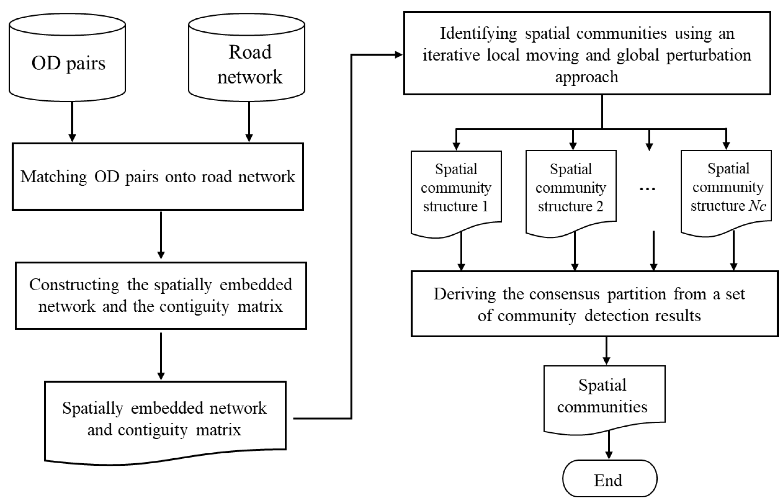
The study area was within the fifth ring road of Beijing (Figure 1). The road network within the study area consists of 10,919 road segments. In this study, the taxi GPS trajectory data was collected on 16 May 2016, (Monday) and 22 May 2016, (Sunday), covering approximately, 30,000 taxis. Each trajectory contains the records of taxi ID, location, time, length, velocity, sampling time, and passenger state. The OD points of vehicle trajectories were mapped onto their nearest road segments [37]. We detected the spatial communities during morning rush hours (7:00–9:00) and afternoon rush hours (16:00–19:00). On Monday, there are 34,604 and 46,677 OD pairs during the morning and afternoon rush hours, respectively. On Sunday, there were 20,520 and 34,361 OD pairs during the morning and afternoon rush hours, respectively.
Detecting spatial communities from these taxi GPS trajectory data is helpful for sensing human mobility patterns and urban structures [10,11]. Existing work has found that spatial communities in vehicle movements are highly related to business centers, transportation hubs, and other popular gathering places [31]. Therefore, 39 highlighted locations were selected to analyze the detected spatial communities. Table 1 lists the detailed descriptions of these locations.

4. Method

The framework of the proposed method is shown in Figure 2. First, we mapped the OD points of vehicle trajectories onto their nearest road segments and constructed a weighted, spatially embedded network. Second, an iterative local moving and global perturbation approach was developed to identify several spatial community detection results. Finally, we performed consensus clustering to generate a more stable and representative spatial community structure out of a set of community detection results.

4.1. Construction of a Weighted Spatially Embedded Network

A weighted spatially embedded network can be defined as G = (V, E, W), where V is the vertex set (a vertex vi refers to a road segment i), E is the edge set (an edge eij refers to the OD pairs between vi and vj), and W is the weight set (the weight wij of each edge corresponds to the number of OD pairs between vi and vj). Two vertices, vi and vj, are spatial neighbors if (1) there is at least one OD pair between vi and vj and (2) vi and vj are topologically adjacent. Figure 3b represents a weighted spatially embedded network constructed based on the road network in Figure 3a, where the letters represent road segments, and the numbers represent the weights of edges. Figure 3c represents the spatial adjacency matrix between road segments. If vi and vj are spatially adjacent, the corresponding position in the adjacency matrix is 1 and 0 otherwise. In this study, a spatial community is defined as a spatially contiguous subgraph of the road network, where OD pairs within that subgraph are significantly more than those between that subgraph and the rest of the road network. In Figure 3b, colored vertices and edges form a spatial community Ci = ( V C i , E C i , W C i ), where V C i = { v A , v B , v D , v E }, E C i = { e A B , e A D , e A E , e B E , e D E }, and W C i = { w A B = 3, w A D = 4, w A E = 5, w B E = 6, w D E = 3}.
In this study, we used modularity to measure the quality of spatial communities [17]. Given a weighted spatially embedded network G and a partitioning C = {C1, C2, …, Cnum}, modularity Q is defined as:
Q = 1 2 m i , j w i j S i S j 2 m δ ( C i , C j )
m is the sum of the edge weights of G, wij is the weight of the edge between vi and vj, S i = j w i j is the strength of the vi, and δ ( C i , C j ) is 1 if C i = C j and 0 otherwise.

4.2. Iterative Local Moving and Global Perturbation Approach

The problem of spatial community identification can be regarded as the optimization problem of modularity. In this study, we developed a new multi-level merging approach, i.e., iterative local moving and global perturbation, to handle the problem of local optimum trap. The iterative local moving and global perturbation approach can be implemented in the following three steps (Figure 4 displays a schematic illustration of the approach):
(1)
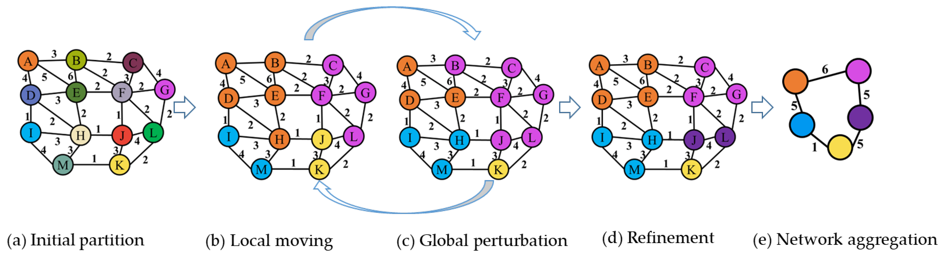
Spatially constrained local moving. We first initialize each vertex as a spatial community (Figure 4a). Then, each vertex vi was moved from the current community to a spatial adjacent community of vi that yields the largest increase in modularity. When modularity cannot be improved by moving each vertex, a local optimum solution is obtained (Figure 4b). Community Cj is a spatial adjacent community of vertex vi if at least one vertex in Cj is the spatial neighbor of vi. The gain of modularity for moving a vertex vi from community Cj to community Ck (jk) can be calculated as:
Δ Q i = k , i n + S i , k 2 m k , t o t + S i 2 m 2 k , i n   2 m k , t o t   2 m 2 + j , i n S i , j 2 m j , t o t S i 2 m 2 j , i n   2 m j , t o t   2 m 2 = 1 2 m S i , k S i , j + S i m j , t o t k , t o t S i
where k , i n and j , i n are the sum of the weights of the edges inside Ck and Cj, respectively. S i , k and S i , j are the sums of the weights of the edges between vi and the vertices in Ck and Cj, respectively. S i is the sum of edge weights linked to vi. k , t o t and j , t o t are the sums of the weights of the edges linked to the vertices in Ck and Cj, respectively. The sum of the edge weights of the network is defined by m;
(2)
Spatially constrained global perturbation. After the local moving operation, we further used a global perturbation operation [38] to reconstruct the local optimum solution. An ideal global perturbation operation should not only jump out of the local optimum trap, but also guide the algorithm to find a possible better solution [27]. To achieve this purpose, for each vertex vi on the boundaries of communities, we first identified the spatial adjacent community of vi, which makes ∆Qi reaches its maximum value. Then, we sorted these vertices in a non-increasing order according to ∆Q. Finally, we selected the first Np vertices to forcibly move them from their original communities to their spatial adjacent communities, even if the ∆Q values are negative (Figure 4c). The spatial continuity of each community cannot be destroyed in the global perturbation process. After the global perturbation, a new round of spatially constrained local moving (Step 1) should be applied to optimize modularity. We performed the global perturbation operation Id times and recorded the community detection result with the highest modularity;
(3)
Refinement and network aggregation. After spatially constrained global perturbation, there may be some weakly-connected (even disconnected) spatial communities. The refinement operation of Leiden [35] was modified to handle this problem. Each spatial community was considered as a sub-network. The spatially constrained local moving method in Step 1 was performed within each sub-network (Figure 4d). A spatial community may be split into several small communities (but not always). After the refinement operation, a network aggregation operation [25] was used to construct a new weighted spatially embedded network, where each vertex is a spatial community and the weights between vertices are the sum of the weights between two communities (Figure 4e).
The above three steps were iteratively implemented until modularity could not be further improved.

4.3. Identification of Stable Spatial Communities Based on Consensus Clustering

The method introduced in Section 4.2 is not deterministic. Multiple runs of the algorithm may produce different results. To handle this problem, consensus clustering was employed to generate a more stable and representative spatial community structure out of a set of community detection results [16,36]. The basic idea is that two vertices are more likely to belong to the same community if they belong to the same community in different partitions. Based on this idea, we first constructed a consensus matrix based on the cooccurrence of vertices in different community detection results. Then, the method in Section 4.2 was performed to identify spatial communities using the consensus matrix.
The consensus matrix D is an N × N matrix, where Dij represents the frequency of vi and vj in the same community, and N is the number of vertices in the weighted spatially embedded network. A large value of Dij indicates that vi and vj frequently appear in the same community. A low value of Dij indicates that vi and vj may be on the boundaries between different communities. To reduce the noise interference and improve the clustering efficiency, we set Dij to 0 if Dij is smaller than a threshold t [36]. A consensus network GC = (V, EC, WC) can be constructed based on the filtered D, where each edge e i j C in the edge set EC refers to the cooccurrence of two vi and vj in the same community, and each weight w i j C in WC corresponds to the frequency of vi and vj in the same community. The spatial community detection method in Section 4.2 was applied to the consensus network Nc times. The consensus clustering operation stops until Nc results discovered from the consensus network are equal.
Figure 5 displays a schematic illustration of the construction of a consensus matrix and consensus network. In Figure 5a, there are three spatial community detection results obtained by the method introduced in Section 4.2. Figure 5b displays the consensus matrix constructed based on the three results in Figure 5a. For example, DAF = 1/3 means that the frequency of vA and vF in the same community is 1/3. The consensus matrix can be further transformed into a consensus network, as shown in Figure 5c. There is an edge between two vertices, vi and vj if D i j > t.

4.4. The Implementation of the Proposed Method

The proposed method requires four parameters: the iteration number of global perturbations Id, the number of perturbation vertices Np, the number of community detection results Nc, and the threshold t. The input data of the proposed method include road networks I and OD pairs of vehicle movements (Trj). The pseudo-code of the proposed method (Algorithm 1) is described as follows.
Algorithm 1SCMiner (Input: R, Trj, Id, Np, Nc, t)
SpatialAdjacencyMatrix = SpatialAdjacencyMatrixConstructiI(R)//Construct the spatial adjacency matrix of the road network
For r = 1: Nc
Network = NetworkConstruction (Trj)//Construct the weighted spatially embedded network
CommunityStructure = InitializeCommunityStructure (Network)//Initialize the spatial community structure
CommunityStructure = SpatiallyConstrainedLocalMoving (CommunityStructure, Network, SpatialAdjacencyMatrix)//Optimize the communities under the contiguity constraint
Flag = True
 while Flag = True:
  For i = 1: Id
   CommunityStructure = SpatiallyConstrainedGlobalPerturbation (CommunityStructure, Network, SpatialAdjacencyMatrix, Np)//Spatially constrained global perturbation
   CommunityStructure = SpatiallyConstrainedLocalMoving (CommunityStructure, Network, SpatialAdjacencyMatrix)//Optimize communities under the contiguity constraint
  End for i
  CommunityStructure = Refinement (CommunityStructure, Network, SpatialAdjacencyMatrix)//Refine the network
  CommunityStructure, Network = NetworkAggregation(CommunityStructure, Network)//Aggregate communities into vertices
  InitialQ = Modularity (CommunityStructure)//Calculate modularity of the spatial community structure
  CommunityStructure = SpatiallyConstrainedLocalMoving (CommunityStructure, Network, SpatialAdjacencyMatrix)//Optimize the communities under the contiguity constraint
  NewQ = Modularity (CommunityStructure)//Calculate modularity of the spatial community structure
  If NewQ = InitialQ:
   Flag = False
 End while
 Insert CommunityStructure into CandidateCommunityStructures
End for r
TrueCommunityStructure = ConsensusClustering (CandidateCommunityStructures, t)//Apply consensus clustering on Nc results
return TrueCommunity
The time and space complexities of the proposed method mainly depend on two elements: (1) The identification of spatial communities using the iterative local moving and global perturbation approach, the time complexity does not exceed O( N c i d N n e i N l o g ( N ) ) and the space complexity is approximately O(N), where Nnei is the mean number of the neighboring communities for each vertex; (2) The identification of stable spatial community structure using consensus clustering, the time complexity does not exceed O( i c N c i d N n e i N l o g ( N ) ), and the space complexity is approximately O(N), where I c is the iteration number of consensus clustering. The total time complexity of the proposed method is approximately O( i c N c i d N n e i N l o g ( N ) ), and the total space complexity of the proposed method is approximately O(N).

5. Experimental Results

The proposed method was compared with a state-of-the-art method—Scleiden [9]. To make a fair comparison between these two methods, we also used consensus clustering to generate a more stable spatial community structure out of a set of community detection results obtained by Scleiden. We named this consensus Scleiden algorithm as Scleiden+. All the methods were implemented in Python 3.7 on a workstation with a 2.20 GHz computer processing unit and 32 GB of memory running the Microsoft Windows 10 operating system. The code for Scleiden was provided by the authors of the original paper.

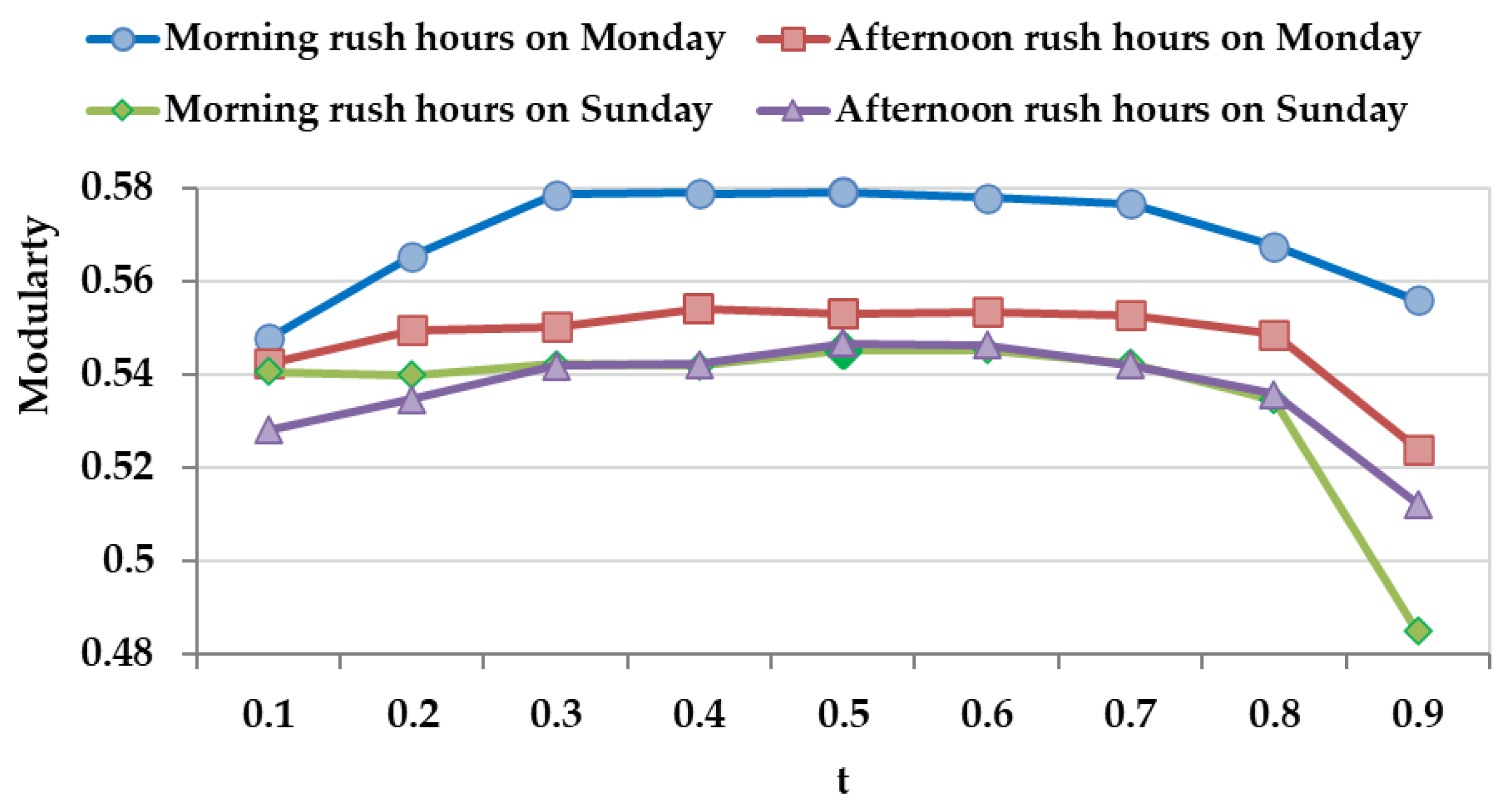
5.1. Parameters Setting

For Scleiden, the threshold of community size was set to 100 and the resolution parameter was set to 1. For the proposed method, we empirically set Np = n/5 and Nc = 20 [27,36], where n is the number of vertices on the boundary of each of the two communities. We have evaluated how the modularity value varied with the iteration number of global perturbations Id. In Figure 6, one can find that the modularity value does not increase obviously with the increase of Id. To balance the quality and efficiency of the proposed method, we set Id = 20 in this study. We also investigated the effect of the filtering threshold (t) on the spatial community quality (Figure 7). One can find that the modularity value usually reaches its maximum when t = 0.5. Therefore, we set t to 0.5 in this study.
In this study, we used modularity to evaluate the quality of spatial communities. It has been proven that modularity optimization has a resolution limit [39]. To maximize modularity value, some small communities cannot be identified. To identify spatial communities with a high resolution, we recursively applied each method to divide a spatial community Ci into sub-communities if the modularity value of Ci is greater than a threshold Qmin [40]. Most real-world networks have Q ≥ 0.3 [41]; therefore, Qmin was set to 0.35 in this study.
Consensus clustering was applied to get a stable result. We have tested how the stability of the results varied with the iteration number (i.e., Ic) of consensus clustering. In each iteration, we measured the consistency of Nc results using the mean of the Normalized Mutual Information (NMI) [42] of each two results in the Nc results. Figure 8 shows the variation of NMI with Ic. A stable result can be obtained when Ic = 2.

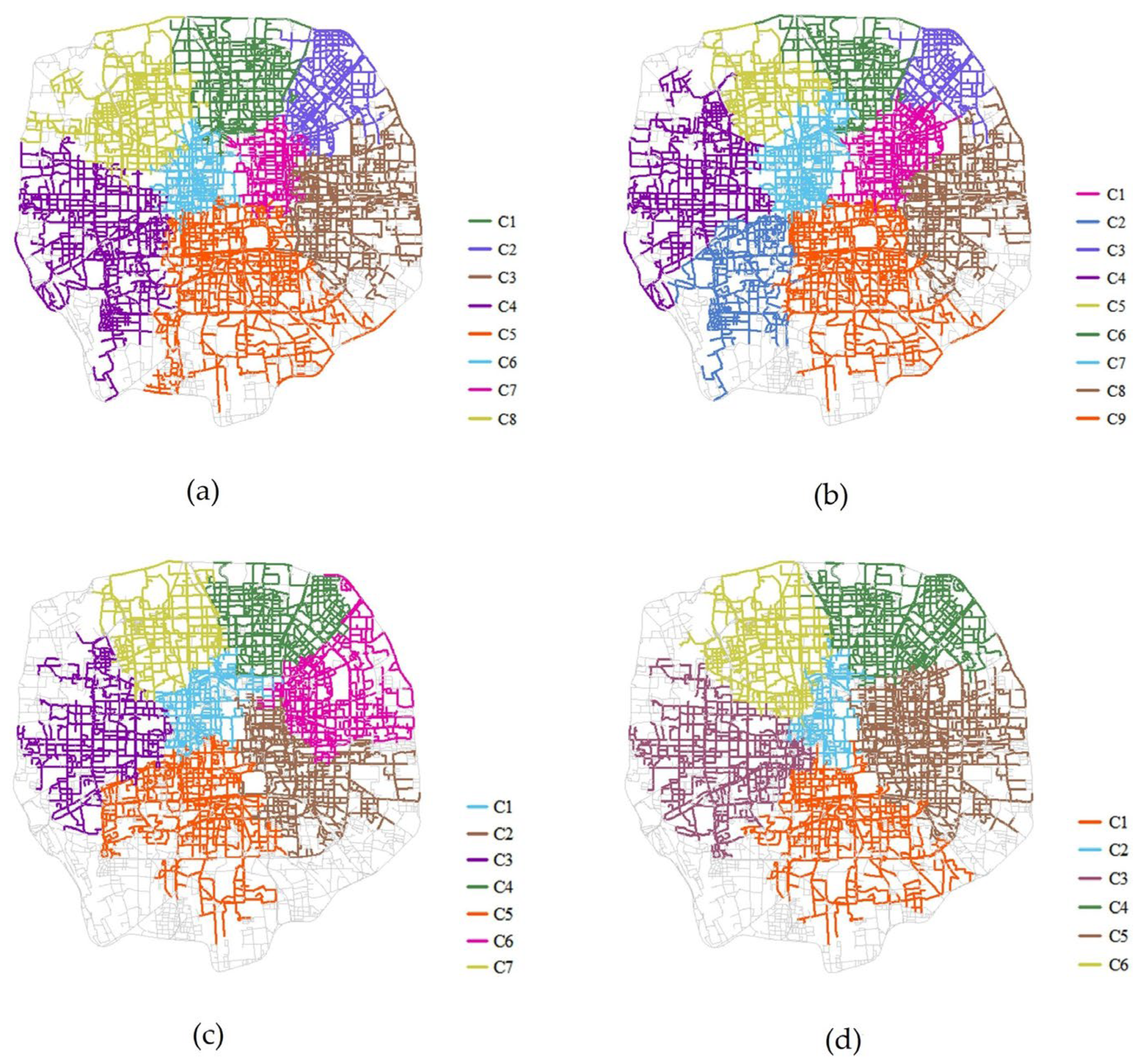
5.2. Spatial Communities during Morning Rush Hours

Figure 9 shows the low-resolution spatial communities discovered by the proposed method and Scleiden+ during the morning rush hours on Monday and Sunday. Figure 10 shows the high-resolution spatial communities discovered by these two methods. From Figure 9, we can find that low-resolution spatial communities discovered by these two methods are similar. However, the spatial ranges of some communities identified by the two methods are different. From Figure 10, one can find that there are obviously differences between the high-resolution spatial communities identified by these two methods. We used the average frequency of OD pairs between road segments within the same community (named the AF index) to quantitatively evaluate the quality of each community [2]. A densely connected community has a high value in the AF index. The AF index values of the communities identified by these two methods are listed in Table 2. One can find that the proposed method performs better in identifying compact communities.
Modularity was also used to quantitatively compare these two methods. The modularity values of the spatial communities detected by these two methods are listed in Table 3. We also ran Scleiden 20 times and calculated the average modularity values of the 20 results (the third column in Table 3). One can find that the modularity values of the spatial communities detected by the proposed method are the highest. Therefore, we can conclude that the proposed method performs better than Scleiden and Scleiden+ in detecting spatial communities during the morning rush hours.

5.3. Spatial Communities during Afternoon Rush Hours

The low-resolution spatial communities discovered by the proposed method and Scleiden+ during afternoon rush hours are displayed in Figure 11. Figure 12 shows the high-resolution spatial communities discovered by these two methods. We can find that the spatial communities identified by these two methods have obvious differences during the afternoon rush hours. The AF index values of the communities identified by these two methods are listed in Table 4. The results show that the communities identified by the proposed method are more compact than those identified by Scleiden+. Comparing Figure 11a with Figure 11b, it can be found that the proposed method identified a community (C1 whose AF index value is 6.8) in the city center on Monday; however, Scleiden+ divided C1 into different communities. From Table 4, we can find that the segmentation of C1 leads to the decrease of community compactness.
Modularity was also used to quantitatively evaluate the performance of the three methods. The third column in Table 5 shows the average modularity values of the 20 results obtained by Scleiden. From Table 5, one can find that the modularity values of the spatial communities identified by the proposed method are the highest.

6. Discussion

The experimental results on the taxi GPS trajectory data in Beijing show that the proposed method outperforms Scleiden and Scleiden+ in detecting spatial communities. The primary reasons for this can be analyzed as follows:
(i) The global perturbation strategy used by the proposed method is efficient for jumping out of the local optimum trap. Therefore, the quality of the communities identified by the iterative local moving and global perturbation approaches can be improved. In contrast, for Scleiden, the local optimum solution obtained in the initial partition step will reduce the quality of the final community identification;
(ii) Consensus clustering, used by the proposed method, is helpful for improving the stability of the identified spatial community structure. The information from different community detection results can reduce the uncertainty of the proposed method caused by the choice of initial conditions. The proposed method performs better than Scleiden+ because the quality of spatial communities identified by the iterative local moving and global perturbation approaches is superior to that identified by Scleiden.
The spatial communities identified from Beijing taxi trajectory data are helpful for sensing the polycentric structure of Beijing. Compared to traditional methods that rely on statistical data (e.g., population census and economic data), the spatial communities in vehicle movements can describe the actual dynamics of human activities in a city [43]. We overlapped the highlighted locations in Figure 1 with the identified spatial communities to analyze the polycentric structure of Beijing (Figure 13 and Figure 14). One can find that some identified spatial communities are similar to the administrative district partitions (Figure 1). The distribution of spatial communities is closely related to business centers and transportation hubs, which indicates that spatial interactions around these places are strong. The identified spatial communities may be used to identify the service areas of different business centers. When we compare Figure 13 and Figure 14, we can see that the spatial community structures identified on workdays and weekends differ. The number of spatial communities on a workday is greater than that on a weekend. The range of the spatial community structure on a workday is wider than that on a weekend. It indicates that different human mobility patterns on weekdays and weekends shape different structures in a city.
The spatial communities identified by the proposed method can be further used to analyze the regional characteristics of human mobility patterns. Table 3 and Table 5 show that the modularity values of the spatial communities identified during the workday are higher than those during the weekend. The reason may be that the intensity of human activities on workday is stronger than that on weekends and the range of human mobility on workday is wider than that on weekend. In the following, we give some examples to illustrate the differences in human mobility patterns on weekday and weekend.
During morning rush hours, two large spatial communities in Regions A and C on Monday (Figure 13a) were divided into several smaller ones on Sunday (Figure 13b). Region A includes Xidan, Financial Street, and Xizhimen. Region C includes Wangfujing, Zhaowai, Dongzhimen, and Beijing Railway Station. These two regions contain many shopping malls and tourist attractions, as well as a transportation hub, which leads to huge crowds and traffic jams on the weekends. Therefore, people are not inclined to choose long trips. Correspondingly, small communities were identified in Regions A and C on Sunday. In Region B, two small communities on Monday (Figure 13a) were merged into one large community on Sunday (Figure 13b). Region B includes Beijing University of Aeronautics and Astronautics, the University of Science and Technology Beijing, and Beitaipingzhuang. On workdays, students tend to move around the universities. On weekends, the scope of students’ activities expands, and many tourists also visit the two colleges. As a result, spatial interactions in Region B became strong on the weekend (only one community was identified on the weekend).
During afternoon rush hours, a large spatial community in Region A on Monday (Figure 14a) was split into two small communities on Sunday (Figure 14b). Region A comprises many residential areas and office buildings. On workdays, the commutes of urban residents enhance the spatial interaction in Region A; therefore, only one large spatial community was discovered on Monday. On the weekend, people in different neighborhoods tend to move near their homes. Correspondingly, the interactions between the two communities in region A (Figure 14b) on Sunday become weak. In Region B, two small communities on Monday (Figure 14a) were merged into one large community on Sunday (Figure 14b). Region B includes a famous business district, Wangjing. On weekends, many people go to Wangjing for entertainment and shopping. Therefore, the spatial interactions between Wangjing and its surrounding areas have become strong.
We can find that the spatial communities identified by the proposed method are useful for sensing urban polycentric structures and human mobility patterns, which can help urban planners understand how human mobility shapes the structure of a city. The spatial communities identified by the proposed method are more accurate and stable than the comparison methods. Therefore, we can infer that the proposed method is a useful urban sensing technique that can empower advanced analytics solutions for urban planners. In this study, we only used the taxi GPS trajectory data collected in 2016 to evaluate the effectiveness and practicability of the proposed method. The proposed method can be further used to analyze the effect of the COVID-19 epidemic on human mobility. For example, we can compare the spatial communities identified before the pandemic, during the pandemic, and after the pandemic. Unfortunately, due to privacy protection, we cannot obtain the taxi GPS trajectory data from 2020 to 2022. Therefore, we leave this research question for future work.

7. Conclusions

In this study, we proposed a hybrid heuristic algorithm by combining multi-level merging and consensus clustering to detect spatial communities in vehicle movements. The proposed method can effectively alleviate two thorny problems of spatial community detection, i.e., problems of local optimality and unstable results. Specifically, we used a global perturbation operation to jump out of the local optimum trap; therefore, the quality of the community detection results can be improved. We employed the consensus clustering strategy to identify a more stable and representative spatial community structure from vehicle movements, which can reduce the uncertainty in real applications. Moreover, the proposed method does not require users to set the number of communities. As a result, users can easily implement the proposed method in practice. Experiments on Beijing taxi trajectory data showed that the proposed method outperforms Scleiden. The proposed method is recommended as a powerful tool for solving the regionalization problems, such as the delineation of neighborhood boundaries [7], the definition of function regions [9], and the identification of urban structures [31].
The proposed method is only designed for detecting spatial communities in a single type of vehicle movement. To obtain a comprehensive view of urban structure and human mobility patterns in a city, we suggest applying the proposed method to identify spatial communities from different types of vehicle movement data, e.g., taxi GPS trajectories and bus/metro smart card transactions. By comparing the spatial communities identified from different types of vehicle movement data, we can deeply understand the relationship between different traffic modes and how different traffic modes shape the structure of a city [11]. The proposed method also has two limitations. First, the efficiency of the proposed method is lower than that of the existing methods because the consensus clustering strategy needs to execute the iterative local moving and global perturbation approach several times. Second, the dynamics of spatial communities cannot be revealed by the proposed method. Therefore, we cannot discover how these spatial communities change over time. In the future, we will extend the proposed method to identify dynamic spatial communities that are useful for understanding the dynamical organization of urban space.

Author Contributions

Conceptualization, Q.L. and J.Y.; methodology, Q.L. and Z.H.; software, Z.H.; validation, Z.H. and J.Y.; formal analysis, Z.H. and Q.L.; investigation, Q.L. and J.Y.; resources, Q.L. and Z.H.; data curation, Z.H.; writing—original draft preparation, Z.H. and J.Y.; writing—review and editing, Q.L.; visualization, Z.H.; supervision, Q.L. and J.Y.; project administration, Q.L.; funding acquisition, Q.L. All authors have read and agreed to the published version of the manuscript.

Funding

This research was funded through support from the National Natural Science Foundation of China (NSFC) (No. 41971353 and 41730105), Natural Science Foundation of Hunan Province (No. 2021JJ20058 and 2020JJ4695), and the water conservancy science and technology project of Guizhou Province (No. KT202110 and KT202002).

Data Availability Statement

Not applicable.

Acknowledgments

The authors gratefully acknowledge the comments from the reviewers.

Conflicts of Interest

The authors declare no conflict of interest.

References

  1. Siła-Nowicka, K.; Vandrol, J.; Oshan, T.; Long, J.A.; Demšar, U.; Fotheringham, A.S. Analysis of human mobility patterns from GPS trajectories and contextual information. Int. J. Geogr. Inf. Sci. 2015, 30, 881–906. [Google Scholar] [CrossRef] [Green Version]
  2. Liu, K.; Gao, S.; Lu, F. Identifying spatial interaction patterns of vehicle movements on urban road networks by topic modelling. Comput. Environ. Urban Syst. 2019, 74, 50–61. [Google Scholar] [CrossRef]
  3. Zhu, D.; Wang, N.; Wu, L.; Liu, Y. Street as a big geo-data assembly and analysis unit in urban studies: A case study using Beijing taxi data. Appl. Geogr. 2017, 86, 152–164. [Google Scholar] [CrossRef]
  4. Liu, X.; Gong, L.; Gong, Y.; Liu, Y. Revealing travel patterns and city structure with taxi trip data. J. Transp. Geogr. 2015, 43, 78–90. [Google Scholar] [CrossRef] [Green Version]
  5. Zheng, Y.; Capra, L.; Wolfson, O.; Yang, H. Urban computing: Concepts, methodologies, and applications. ACM Trans. Intell. Syst. Technol. TIST 2014, 5, 1–55. [Google Scholar] [CrossRef]
  6. Liu, Y.; Liu, X.; Gao, S.; Gong, L.; Kang, C.; Zhi, Y.; Chi, G.; Shi, L. Social sensing: A new approach to understanding our socioeconomic environments. Ann. Assoc. Am. Geogr. 2015, 105, 512–530. [Google Scholar] [CrossRef]
  7. Guo, D.; Jin, H.; Gao, P.; Zhu, X. Detecting spatial community structure in movements. Int. J. Geogr. Inf. Sci. 2018, 32, 1326–1347. [Google Scholar] [CrossRef]
  8. Chen, Y.; Xu, J.; Xu, M. Finding community structure in spatially constrained complex networks. Int. J. Geogr. Inf. Sci. 2015, 29, 889–911. [Google Scholar] [CrossRef]
  9. Wang, C.; Wang, F.; Onega, T. Network Optimization Approach to Delineating Health Care Service Areas: Spatially Constrained Louvain and Leiden Algorithms. Trans. GIS 2021, 25, 1065–1081. [Google Scholar] [CrossRef]
  10. Zhong, C.; Arisona, S.M.; Huang, X.; Batty, M.; Schmitt, G. Detecting the dynamics of urban structure through spatial network analysis. Int. J. Geogr. Inf. Sci. 2014, 28, 2178–2199. [Google Scholar] [CrossRef]
  11. Zhang, X.; Xu, Y.; Tu, W.; Ratti, C. Do different datasets tell the same story about urban mobility—A comparative study of public transit and taxi usage. J. Transp. Geogr. 2018, 70, 78–90. [Google Scholar] [CrossRef]
  12. Lu, F.; Liu, K.; Duan, Y.; Cheng, S.; Du, F. Modeling the heterogeneous traffic correlations in urban road systems using traffic-enhanced community detection approach. Phys. A Stat. Mech. Appl. 2018, 501, 227–237. [Google Scholar] [CrossRef]
  13. Fortunato, S. Community detection in graphs. Phys. Rep. 2010, 486, 75–174. [Google Scholar] [CrossRef] [Green Version]
  14. Attea, B.A.A.; Abbood, A.D.; Hasan, A.A.; Pizzuti, C.; Al-Ani, M.; Özdemir, S.; Al-Dabbagh, R.D. A review of heuristics and metaheuristics for community detection in complex networks: Current usage, emerging development and future directions. Swarm Evol. Comput. 2021, 63, 100885. [Google Scholar] [CrossRef]
  15. Rossetti, G.; Cazabet, R. Community discovery in dynamic networks: A survey. ACM Comput. Surv. 2018, 51, 1–37. [Google Scholar] [CrossRef] [Green Version]
  16. Strehl, A.; Ghosh, J. Cluster ensembles-a knowledge reuse framework for combining multiple partitions. J. Mach. Learn. Res. 2002, 3, 583–617. [Google Scholar]
  17. Newman, M.E.; Girvan, M. Finding and evaluating community structure in networks. Phys. Rev. E 2004, 69, 026113. [Google Scholar] [CrossRef] [Green Version]
  18. Clauset, A.; Newman, M.E.; Moore, C. Finding community structure in very large networks. Phys. Rev. E 2004, 70, 066111. [Google Scholar] [CrossRef] [Green Version]
  19. Chakraborty, T.; Dalmia, A.; Mukherjee, A.; Ganguly, N. Metrics for community analysis: A survey. ACM Comput. Surv. (CSUR) 2017, 50, 1–37. [Google Scholar] [CrossRef]
  20. Cafieri, S.; Hansen, P.; Liberti, L. Edge ratio and community structure in networks. Phys. Rev. E Stat. Nonlinear Soft Matter Phys. 2010, 81, 026105. [Google Scholar] [CrossRef] [Green Version]
  21. Radicchi, F.; Castellano, C.; Cecconi, F.; Loreto, V.; Parisi, D. Defining and identifying communities in networks. Proc. Natl. Acad. Sci. USA 2004, 101, 2658–2663. [Google Scholar] [CrossRef] [Green Version]
  22. Shi, J.; Malik, J. Normalized cuts and image segmentation. IEEE Trans. Pattern Anal. Mach. Intell. 2000, 22, 888–905. [Google Scholar]
  23. Rosvall, M.; Bergstrom, C.T. Maps of random walks on complex networks reveal community structure. Proc. Natl. Acad. Sci. USA 2008, 105, 1118–1123. [Google Scholar] [CrossRef] [Green Version]
  24. Rosvall, M.; Bergstrom, C.T. Multilevel compression of random walks on networks reveals hierarchical organization in large integrated systems. PLoS ONE 2011, 6, e18209. [Google Scholar] [CrossRef] [Green Version]
  25. Blondel, V.D.; Guillaume, J.-L.; Lambiotte, R.; Lefebvre, E. Fast unfolding of communities in large networks. J. Stat. Mech. Theory Exp. 2008, 2008, P10008. [Google Scholar] [CrossRef] [Green Version]
  26. Gach, O.; Hao, J.-K. Combined neighborhood tabu search for community detection in complex networks. RAIRO-Oper. Res. 2016, 50, 269–283. [Google Scholar] [CrossRef] [Green Version]
  27. Lu, Z.; Huang, W. Iterated tabu search for identifying community structure in complex networks. Phys. Rev. E Stat. Nonlinear Soft Matter Phys. 2009, 80, 026130. [Google Scholar] [CrossRef]
  28. Pons, P.; Latapy, M. Computing communities in large networks using random walks. In Proceedings of the 20th International Symposium on Computer and Information Sciences, Istanbul, Turkey, 26–28 October 2005; pp. 284–293. [Google Scholar]
  29. Karimi, F.; Lotfi, S.; Izadkhah, H. Multiplex community detection in complex networks using an evolutionary approach. Expert Syst. Appl. 2020, 146, 113184. [Google Scholar] [CrossRef]
  30. Zhou, X.; Liu, Y.; Zhang, J.; Liu, T.; Zhang, D. An ant colony based algorithm for overlapping community detection in complex networks. Phys. A Stat. Mech. Appl. 2015, 427, 289–301. [Google Scholar] [CrossRef]
  31. Liu, Q.; Zhu, S.; Deng, M.; Liu, W.; Wu, Z. A Spatial Scan Statistic to Detect Spatial Communities of Vehicle Movements on Urban Road Networks. Geogr. Anal. 2021, 54, 124–148. [Google Scholar] [CrossRef]
  32. Expert, P.; Evans, T.S.; Blondel, V.D.; Lambiotte, R. Uncovering space-independent communities in spatial networks. Proc. Natl. Acad. Sci. USA 2011, 108, 7663–7668. [Google Scholar] [CrossRef] [Green Version]
  33. Gao, S.; Liu, Y.; Wang, Y.; Ma, X. Discovering Spatial Interaction Communities from Mobile Phone Data. Trans. GIS 2013, 17, 463–481. [Google Scholar] [CrossRef] [Green Version]
  34. Wan, Y.; Liu, Y. DASSCAN: A Density and Adjacency Expansion-Based Spatial Structural Community Detection Algorithm for Networks. ISPRS Int. J. Geo-Inf. 2018, 7, 159. [Google Scholar] [CrossRef] [Green Version]
  35. Traag, V.A.; Waltman, L.; van Eck, N.J. From Louvain to Leiden: Guaranteeing well-connected communities. Sci. Rep. 2019, 9, 5233. [Google Scholar] [CrossRef]
  36. Lancichinetti, A.; Fortunato, S. Consensus clustering in complex networks. Sci. Rep. 2012, 2, 336. [Google Scholar] [CrossRef]
  37. White, C.E.; Bernstein, D.; Kornhauser, A.L. Some map matching algorithms for personal navigation assistants. Transp. Res. Part C Emerg. Technol. 2000, 8, 91–108. [Google Scholar] [CrossRef]
  38. Lourenço, H.R.; Martin, O.C.; Stützle, T. Iterated local search. In Handbook of Metaheuristics; Springer: Berlin, Germany, 2003; pp. 320–353. [Google Scholar]
  39. Reichardt, J.; Bornholdt, S. Statistical mechanics of community detection. Phys. Rev. E Stat. Nonlinear Soft Matter Phys. 2006, 74, 016110. [Google Scholar] [CrossRef] [Green Version]
  40. Ruan, J.; Zhang, W. Identifying network communities with a high resolution. Phys. Rev. E 2008, 77, 016104. [Google Scholar] [CrossRef] [Green Version]
  41. Newman, M.E. The structure and function of complex networks. SIAM Rev. 2003, 45, 167–256. [Google Scholar] [CrossRef] [Green Version]
  42. Danon, L.; Díaz-Guilera, A.; Duch, J.; Arenas, A. Comparing community structure identification. J. Stat. Mech. Theory Exp. 2005, 2005, P09008. [Google Scholar] [CrossRef]
  43. Cai, J.; Huang, B.; Song, Y. Using multi-source geospatial big data to identify the structure of polycentric cities. Remote Sens. Environ. 2017, 202, 210–221. [Google Scholar] [CrossRef]
Figure 1. Overview of the study area.
Remotesensing 14 04144 g001
Figure 2. Framework of the proposed method.
Remotesensing 14 04144 g002
Figure 3. Construction of a weighted spatially embedded network: (a) road network and an OD pair; (b) the weighted spatially embedded network; and (c) spatial adjacency matrix.
Remotesensing 14 04144 g003
Figure 4. Schematic illustration of the iterative local moving and global perturbation approach: (a) initial partition; (b) local moving; (c) global perturbation; (d) refinement; (e) network aggregation.
Remotesensing 14 04144 g004
Figure 5. Construction of consensus matrix and consensus network: (a) three spatial community detection results; (b) consensus matrix; (c) consensus network.
Remotesensing 14 04144 g005
Figure 6. Modularity with the iteration number of global perturbations.
Remotesensing 14 04144 g006
Figure 7. Modularity with the filtering threshold in consensus clustering.
Remotesensing 14 04144 g007
Figure 8. NMI with different iteration times of consensus clustering.
Remotesensing 14 04144 g008
Figure 9. Low-resolution spatial communities discovered by two methods during morning rush hours: (a) spatial communities identified by the proposed method on Monday; (b) spatial communities identified by Scleiden+ on Monday; (c) spatial communities identified by the proposed method on Sunday; (d) spatial communities identified by Scleiden+ on Sunday.
Remotesensing 14 04144 g009
Figure 10. High-resolution spatial communities discovered by the two methods during morning rush hours: (a) spatial communities identified by the proposed method on Monday; (b) spatial communities identified by Scleiden+ on Monday; (c) spatial communities identified by the proposed method on Sunday; and (d) spatial communities identified by Scleiden+ on Sunday.
Remotesensing 14 04144 g010
Figure 11. Low-resolution spatial communities discovered by the two methods during afternoon rush hours: (a) spatial communities identified by the proposed method on Monday; (b) spatial communities identified by Scleiden+ on Monday; (c) spatial communities identified by the proposed method on Sunday; and (d) spatial communities identified by Scleiden+ on Sunday.
Remotesensing 14 04144 g011
Figure 12. High-resolution spatial communities discovered by the two methods during afternoon rush hours: (a) spatial communities identified by the proposed method on Monday; (b) spatial communities identified by Scleiden+ on Monday; (c) spatial communities identified by the proposed method on Sunday; and (d) spatial communities identified by Scleiden+ on Sunday.
Remotesensing 14 04144 g012
Figure 13. Overlapping results of spatial community during the morning rush hours and highlighted places: (a) spatial communities discovered on Monday; (b) spatial communities discovered on Sunday.
Remotesensing 14 04144 g013
Figure 14. The overlapping results of spatial communities during afternoon rush hours and highlighted places: (a) spatial communities discovered on Monday; (b) spatial communities discovered on Sunday.
Remotesensing 14 04144 g014
Table 1. Descriptions of the highlighted locations in Figure 1.
Description of LocationsName of Locations
Primary business districtA1: Financial Street, A2: Xidan, A3: Wangfujing, A4: Dongzhimen, A5: Sanlitun, A6: Yansha, A7: CBD, A8: Wangjing
Secondary business districtB1: Chongwenmen, B2: Zhaowai, B3: Shuangjing, B4: Gongzhufen, B5: Xizhimen, B6: Taiyanggong, B7: Chaoqing, B8: Yaao, B9: Wanliu, B10: Zhongguancun
Other business districtC1: Guanganmen, C2: Jishuitan, C3: Andingmen, C4: Beitaipingzhuang, C5: Lize, C6: Muxiyuan, C7: Fangzhuang, C8: Panjiayuan, C9: Guangqvmen, C10: Jianguomen, C11: Chaoyang Park, C12: Wukesong, C13: Lugu
CollegeD1: Peking University, D2: Tsinghua University, D3: Beijing University of Aeronautics and Astronautics, D4: University of Science and Technology Beijing
Railway StationE1: Beijing West Railway Station, E2: Beijing South Railway Station, E3: Beijing Station
Tourist spotF1: Tiananmen
Table 2. AF index values of the spatial communities identified by the proposed method and Scleiden+ during morning rush hours.
The Proposed MethodScleiden+
Maximum ValueMinimum ValueAverage ValueMaximum ValueMinimum ValueAverage Value
low resolution results on Monday9.75.47.09.05.16.5
high resolution results on Monday9.01.14.98.00.94.5
low resolution results on Sunday7.43.74.86.72.64.3
high resolution results on Sunday6.11.62.95.11.32.7
Table 3. Modularity values of the spatial communities identified by the proposed method, Scleiden, and Scleiden+ during morning rush hours.
The Proposed MethodScleidenScleiden+
low resolution results on Monday0.5790.5680.568
high resolution results on Monday0.4780.4190.429
low resolution results on Sunday0.5450.5270.529
high resolution results on Sunday0.4220.3750.370
Table 4. AF index values of the spatial communities identified by the proposed method and Scleiden+ during afternoon rush hours.
The Proposed MethodScleiden+
Maximum ValueMinimum ValueAverage ValueMaximum ValueMinimum ValueAverage Value
low resolution results on Monday12.66.29.011.25.98.9
high resolution results on Monday12.72.96.111.92.35.7
low resolution results on Sunday9.84.87.09.74.26.4
high resolution results on Sunday10.32.14.58.81.64.1
Table 5. Modularity values of the spatial communities identified by the proposed method, Scleiden, and Scleiden+ during afternoon rush hours.
The Proposed MethodScleidenScleiden+
low resolution results on Monday0.5540.5430.540
high resolution results on Monday0.4210.4010.407
low resolution results on Sunday0.5460.5380.539
high resolution results on Sunday0.4120.4060.405
Publisher’s Note: MDPI stays neutral with regard to jurisdictional claims in published maps and institutional affiliations.

