
Quantifying the Relationship between 2D/3D Building Patterns and Land Surface Temperature: Study on the Metropolitan Shanghai


 , ,
, ,
Abstract
:
1. Introduction
2. Materials and Methods
2.1. Study Area
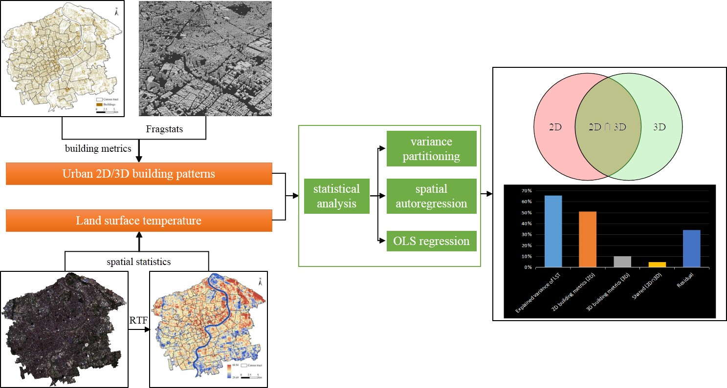
2.2. Methods
2.2.1. Retrieving LST
2.2.2. Measuring 2D/3D Building Patterns
2.2.3. Statistics Analysis
3. Results
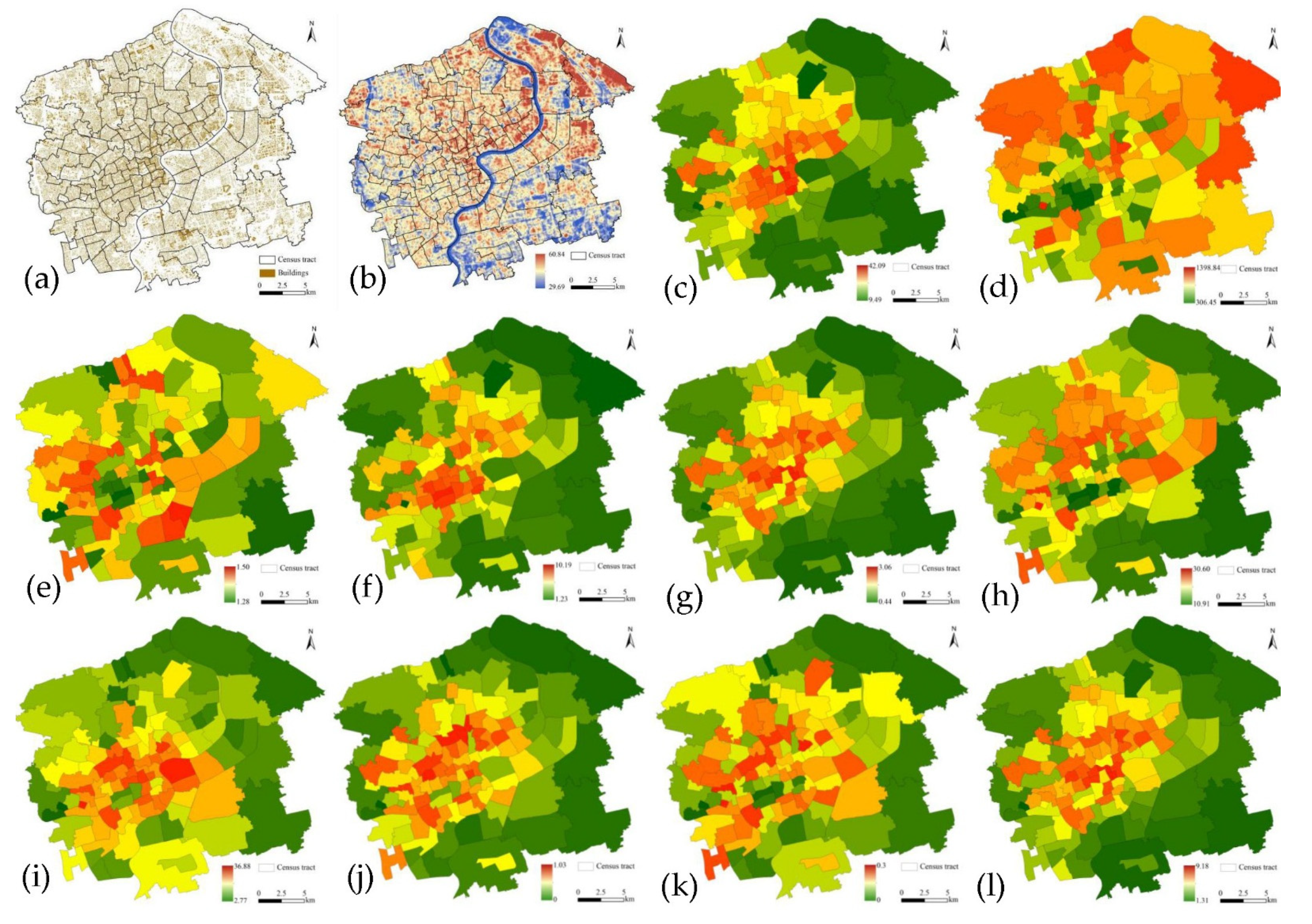
3.1. The Spatial Pattern of Buildings and LST
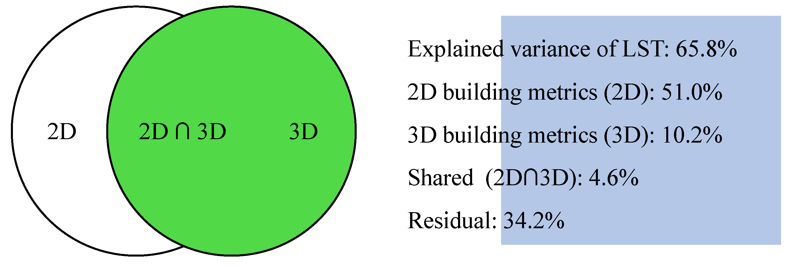
3.2. Relative Importance of 2D/3D Building Metrics in Determining the Variability of LST
4. Discussion
4.1. On the Associations between 2D/3D Building Spatial Patterns and LST
4.2. The Methodical Implications
4.3. Implications of Urban Planning and Management
5. Conclusions
Author Contributions
Funding
Data Availability Statement
Acknowledgments
Conflicts of Interest
References
- Peng, J.; Xie, P.; Liu, Y.; Ma, J. Urban thermal environment dynamics and associated landscape pattern factors: A case study in the Beijing metropolitan region. Remote Sens. Environ. 2016, 173, 145–155. [Google Scholar] [CrossRef]
- Rhee, J.; Park, S.; Lu, Z. Relationship between land cover patterns and surface temperature in urban areas. GISci. Remote Sens. 2014, 51, 521–536. [Google Scholar] [CrossRef]
- Oke, T.R. The energetic basis of the urban heat island. Q. J. R. Meteorol. Soc. 1982, 108, 1–24. [Google Scholar] [CrossRef]
- Taha, H. Urban climates and heat islands: Albedo, evapotranspiration, and anthropogenic heat. Energy Build. 1997, 25, 99–103. [Google Scholar] [CrossRef] [Green Version]
- Voogt, J.A.; Oke, T.R. Thermal remote sensing of urban climates. Remote Sens. Environ. 2003, 86, 370–384. [Google Scholar] [CrossRef]
- Weng, Q.; Yang, S. Urban air pollution patterns, land use, and thermal landscape: An examination of the linkage using GIS. Environ. Monit. Assess. 2006, 117, 463–489. [Google Scholar] [CrossRef] [PubMed]
- Grimm, N.B.; Faeth, S.H.; Golubiewski, N.E.; Redman, C.L.; Wu, J.; Bai, X.; Briggs, J.M. Global change and the ecology of cities. Science 2008, 319, 756–760. [Google Scholar] [CrossRef] [Green Version]
- Gober, P.; Brazel, A.; Quay, R.; Myint, S.; Grossman-Clarke, S.; Miller, A.; Rossi, S. Using watered landscapes to manipulate urban heat island effects: How much water will it take to cool Phoenix? J. Am. Plan. Assoc. 2009, 76, 109–121. [Google Scholar] [CrossRef]
- Konopacki, S.; Akbari, H. Energy Savings for Heat Island Reduction Strategies in Chicago and Houston (Including Updates for Baton Rouge, Sacramento, and Salt Lake City); University of California: Berkeley, CA, USA, 2002. [Google Scholar]
- Wan, K.K.; Li, D.H.; Pan, W.; Lam, J.C. Impact of climate change on building energy use in different climate zones and mitigation and adaptation implications. Appl. Energy 2012, 97, 274–282. [Google Scholar] [CrossRef]
- Santamouris, M.; Cartalis, C.; Synnefa, A.; Kolokotsa, D. On the impact of urban heat island and global warming on the power demand and electricity consumption of buildings—A review. Energy Build. 2015, 98, 119–124. [Google Scholar] [CrossRef]
- White, M.A.; Nemani, R.R.; Thornton, P.E.; Running, S.W. Satellite evidence of phenological differences between urbanized and rural areas of the eastern United States deciduous broadleaf forest. Ecosystems 2002, 5, 260–273. [Google Scholar] [CrossRef]
- Niemelä, J. Ecology and urban planning. Biodivers. Conserv. 1999, 8, 119–131. [Google Scholar] [CrossRef]
- Poumadère, M.; Mays, C.; Le Mer, S.; Blong, R. The 2003 heat wave in France: Dangerous climate change here and now. Risk Anal. 2005, 25, 1483–1494. [Google Scholar] [CrossRef] [PubMed]
- Patz, J.A.; Campbell-Lendrum, D.; Holloway, T.; Foley, J.A. Impact of regional climate change on human health. Nature 2005, 438, 310–317. [Google Scholar] [CrossRef] [PubMed]
- Harlan, S.L.; Ruddell, D.M. Climate change and health in cities: Impacts of heat and air pollution and potential co-benefits from mitigation and adaptation. Curr. Opin. Environ. Sustain. 2011, 3, 126–134. [Google Scholar] [CrossRef]
- Jenerette, G.D.; Harlan, S.L.; Buyantuev, A.; Stefanov, W.L.; Declet-Barreto, J.; Ruddell, B.L.; Myint, S.W.; Kaplan, S.; Li, X. Micro-scale urban surface temperatures are related to land-cover features and residential heat related health impacts in Phoenix, AZ USA. Landsc. Ecol. 2016, 31, 745–760. [Google Scholar] [CrossRef]
- Weng, Q. Thermal infrared remote sensing for urban climate and environmental studies: Methods, applications, and trends. ISPRS J. Photogramm. Remote Sens. 2009, 64, 335–344. [Google Scholar] [CrossRef]
- Tian, Y.; Zhou, W.; Qian, Y.; Zheng, Z.; Yan, J. The effect of urban 2D and 3D morphology on air temperature in residential neighborhoods. Landsc. Ecol. 2019, 34, 1161–1178. [Google Scholar] [CrossRef]
- Eludoyin, O.M.; Adelekan, I.; Webster, R.; Eludoyin, A. Air temperature, relative humidity, climate regionalization and thermal comfort of Nigeria. Int. J. Clim. 2013, 34, 2000–2018. [Google Scholar] [CrossRef] [Green Version]
- Zeng, L.; Wardlow, B.D.; Tadesse, T.; Shan, J.; Hayes, M.J.; Li, D.; Xiang, D. Estimation of daily air temperature based on MODIS land surface temperature products over the corn belt in the US. Remote Sens. 2015, 7, 951–970. [Google Scholar] [CrossRef] [Green Version]
- Peng, J.; Jia, J.; Liu, Y.; Li, H.; Wu, J. Seasonal contrast of the dominant factors for spatial distribution of land surface temperature in urban areas. Remote Sens. Environ. 2018, 215, 255–267. [Google Scholar] [CrossRef]
- Zhang, H.; Li, T.-T.; Han, J.-J. Quantifying the relationship between land use features and intra-surface urban heat island effect: Study on downtown Shanghai. Appl. Geogr. 2020, 125, 102305. [Google Scholar] [CrossRef]
- Imhoff, M.L.; Zhang, P.; Wolfe, R.E.; Bounoua, L. Remote sensing of the urban heat island effect across biomes in the continental USA. Remote Sens. Environ. 2010, 114, 504–513. [Google Scholar] [CrossRef] [Green Version]
- Zhou, W.; Wang, J.; Cadenasso, M.L. Effects of the spatial configuration of trees on urban heat mitigation: A comparative study. Remote Sens. Environ. 2017, 195, 1–12. [Google Scholar] [CrossRef]
- Sun, F.; Liu, M.; Wang, Y.; Wang, H.; Che, Y. The effects of 3D architectural patterns on the urban surface temperature at a neighborhood scale: Relative contributions and marginal effects. J. Clean. Prod. 2020, 258, 120706. [Google Scholar] [CrossRef]
- Mildrexler, D.J.; Zhao, M.; Running, S.W. A global comparison between station air temperatures and MODIS land surface temperatures reveals the cooling role of forests. J. Geophys. Res. Earth Surf. 2011, 116, 15. [Google Scholar] [CrossRef]
- Kuang, W.; Dou, Y.; Zhang, C.; Chi, W.; Liu, A.; Liu, Y.; Zhang, R.; Liu, J. Quantifying the heat flux regulation of metropolitan land use/land cover components by coupling remote sensing modeling with in situ measurement. J. Geophys. Res. Atmos. 2015, 120, 113–130. [Google Scholar] [CrossRef]
- Clinton, N.; Gong, P. MODIS detected surface urban heat islands and sinks: Global locations and controls. Remote Sens. Environ. 2013, 134, 294–304. [Google Scholar] [CrossRef]
- Ayansina, A. Seasonality in the daytime and night-time intensity of land surface temperature in a tropical city area. Sci. Total Environ. 2016, 557, 415–424. [Google Scholar]
- Peng, J.; Dan, Y.; Qiao, R.; Liu, Y.; Dong, J.; Wu, J. How to quantify the cooling effect of urban parks? Linking maximum and accumulation perspectives. Remote Sens. Environ. 2021, 252, 112135. [Google Scholar] [CrossRef]
- Oke, T.R. Initial Guidance to Obtain Representative Meteorological Observations at Urban Sites; University of British Columbia: Vancouver, BC, Canada, 2004. [Google Scholar]
- Li, J.; Song, C.; Cao, L.; Zhu, F.; Meng, X.; Wu, J. Impacts of landscape structure on surface urban heat islands: A case study of Shanghai, China. Remote Sens. Environ. 2011, 115, 3249–3263. [Google Scholar] [CrossRef]
- Ma, Q.; Wu, J.; He, C. A hierarchical analysis of the relationship between urban impervious surfaces and land surface temperatures: Spatial scale dependence, temporal variations, and bioclimatic modulation. Landsc. Ecol. 2016, 31, 1139–1153. [Google Scholar] [CrossRef]
- Du, H.; Song, X.; Jiang, H.; Kan, Z.; Wang, Z.; Cai, Y. Research on the cooling island effects of water body: A case study of Shanghai, China. Ecol. Indic. 2016, 67, 31–38. [Google Scholar] [CrossRef]
- Berger, C.; Rosentreter, J.; Voltersen, M.; Baumgart, C.; Schmullius, C.; Hese, S. Spatio-temporal analysis of the relationship between 2D/3D urban site characteristics and land surface temperature. Remote Sens. Environ. 2017, 193, 225–243. [Google Scholar] [CrossRef]
- Huang, X.; Wang, Y. Investigating the effects of 3D urban morphology on the surface urban heat island effect in urban functional zones by using high-resolution remote sensing data: A case study of Wuhan, Central China. ISPRS J. Photogramm. Remote Sens. 2019, 152, 119–131. [Google Scholar] [CrossRef]
- Futcher, J.; Mills, G.; Emmanuel, R.; Korolija, I. Creating sustainable cities one building at a time: Towards an integrated urban design framework. Cities 2017, 66, 63–71. [Google Scholar] [CrossRef] [Green Version]
- Scarano, M.; Mancini, F. Assessing the relationship between sky view factor and land surface temperature to the spatial resolution. Int. J. Remote Sens. 2017, 38, 6910–6929. [Google Scholar] [CrossRef]
- Zheng, Z.; Zhou, W.; Yan, J.; Qian, Y.; Wang, J.; Li, W. The higher, the cooler? Effects of building height on land surface temperatures in residential areas of Beijing. Phys. Chem. Earth 2019, 110, 149–156. [Google Scholar] [CrossRef]
- Zhang, H.; Li, T.; Liu, Y.; Han, J.; Guo, Y. Understanding the contributions of land parcel features to intra-surface urban heat island intensity and magnitude: A study of downtown Shanghai, China. Land Degrad. Dev. 2020, 32, 1353–1367. [Google Scholar] [CrossRef]
- Yu, S.; Chen, Z.; Yu, B.; Wang, L.; Wu, B.; Wu, J.; Zhao, F. Exploring the relationship between 2D/3D landscape pattern and land surface temperature based on explainable eXtreme Gradient Boosting tree: A case study of Shanghai, China. Sci. Total Environ. 2020, 725, 138229. [Google Scholar] [CrossRef]
- Peng, S.; Piao, S.; Ciais, P.; Friedlingstein, P.; Ottle, C.; Bréon, F.-M.; Nan, H.; Zhou, L.; Myneni, R.B. Surface urban heat island across 419 global big cities. Environ. Sci. Technol. 2012, 46, 696–703. [Google Scholar] [CrossRef] [PubMed]
- Yang, Q.; Huang, X.; Tang, Q. The footprint of urban heat island effect in 302 Chinese cities: Temporal trends and associated factors. Sci. Total Environ. 2019, 655, 652–662. [Google Scholar] [CrossRef] [PubMed]
- United Nations. The World’s Cities in 2018; United Nations: New York, NY, USA, 2018. [Google Scholar]
- USGS. Landsat 8 (L8) Data Users Handbook; Department of the Interior, U.S. Geological Survey: Washington, DC, USA, 2016.
- Barsi, J.A.; Barker, J.L.; Schott, J.R. An atmospheric correction parameter calculator for a single thermal band earth-sensing instrument. In Proceedings of the IGARSS 2003. 2003 IEEE International Geoscience and Remote Sensing Symposium, Toulouse, France, 21–25 July 2003; Proceedings (IEEE Cat. No. 03CH37477). IEEE: Manhattan, NY, USA, 2003; pp. 3014–3016. [Google Scholar]
- Weng, Q.; Lu, D.; Schubring, J. Estimation of land surface temperature–vegetation abundance relationship for urban heat island studies. Remote Sens. Environ. 2004, 89, 467–483. [Google Scholar] [CrossRef]
- Sobrino, J.A.; Jiménez-Muñoz, J.C.; Paolini, L. Land surface temperature retrieval from LANDSAT TM 5. Remote Sens. Environ. 2004, 90, 434–440. [Google Scholar] [CrossRef]
- Dash, P.; Göttsche, F.-M.; Olesen, F.-S.; Fischer, H. Land surface temperature and emissivity estimation from passive sensor data: Theory and practice-current trends. Int. J. Remote Sens. 2002, 23, 2563–2594. [Google Scholar] [CrossRef]
- Norman, J.M.; Becker, F. Terminology in thermal infrared remote sensing of natural surfaces. Remote Sens. Rev. 1995, 12, 159–173. [Google Scholar] [CrossRef]
- Barsi, J.A.; Butler, J.J.; Schott, J.R.; Palluconi, F.D.; Hook, S.J. Validation of a web-based atmospheric correction tool for single thermal band instruments. In Optics and Photonics 2005; SPIE: Bellingham, WA, USA, 2005; p. 7. [Google Scholar]
- Alavipanah, S.; Schreyer, J.; Haase, D.; Lakes, T.; Qureshi, S. The effect of multi-dimensional indicators on urban thermal conditions. J. Clean. Prod. 2017, 177, 115–123. [Google Scholar] [CrossRef]
- Liu, M.; Hu, Y.-M.; Li, C. Landscape metrics for three-dimensional urban building pattern recognition. Appl. Geogr. 2017, 87, 66–72. [Google Scholar] [CrossRef]
- Riitters, K.H.; O’Neill, R.V.; Hunsaker, C.T.; Wickham, J.D.; Yankee, D.H.; Timmins, S.P.; Jones, K.B.; Jackson, B.L. A factor analysis of landscape pattern and structure metrics. Landsc. Ecol. 1995, 10, 23–39. [Google Scholar] [CrossRef]
- Li, H.; Wu, J. Use and misuse of landscape indices. Landsc. Ecol. 2004, 19, 389–399. [Google Scholar] [CrossRef] [Green Version]
- Peng, J.; Wang, Y.; Zhang, Y.; Wu, J.; Li, W.; Li, Y. Evaluating the effectiveness of landscape metrics in quantifying spatial patterns. Ecol. Indic. 2010, 10, 217–223. [Google Scholar] [CrossRef]
- McGarigal, K.; Cushman, S.; Neel, M.; Ene, E. FRAGSTATS: Spatial Pattern Analysis Program for Categorical Maps; University of Massachusetts: Amherst, MA, USA, 2012. [Google Scholar]
- Lichstein, J.; Simons, T.; Shriner, S.; Franzreb, K. Spatial autocorrelation and autoregressive models in ecology. Ecol. Monogr. 2002, 72, 445–463. [Google Scholar] [CrossRef]
- Li, X.; Zhou, W.; Ouyang, Z.; Xu, W.; Zheng, H. Spatial pattern of greenspace affects land surface temperature: Evidence from the heavily urbanized Beijing metropolitan area, China. Landsc. Ecol. 2012, 27, 887–898. [Google Scholar] [CrossRef]
- Anselin, L. Exploring Spatial Data with GeoDa™: A Workbook; University of Illinois: Urbana, IL, USA, 2005. [Google Scholar]
- Weng, Q.; Lu, D.; Liang, B. Urban Surface Biophysical Descriptors and Land Surface Temperature Variations. Photogramm. Eng. Remote Sens. 2006, 72, 1275–1286. [Google Scholar] [CrossRef] [Green Version]
- Yan, H.; Fan, S.; Guo, C.; Wu, F.; Zhang, N.; Dong, L. Assessing the effects of landscape design parameters on intra-urban air temperature variability: The case of Beijing, China. Build. Environ. 2014, 76, 44–53. [Google Scholar] [CrossRef]
- Zhou, W.; Huang, G.; Cadenasso, M.L. Does spatial configuration matter? Understanding the effects of land cover pattern on land surface temperature in urban landscapes. Landsc. Urban Plan. 2011, 102, 54–63. [Google Scholar] [CrossRef]
- Anderson, M.J.; Gribble, N.A. Partitioning the variation among spatial, temporal and environmental components in a multivariate data set. Aust. J. Ecol. 1998, 23, 158–167. [Google Scholar] [CrossRef]
- Legendre, P. Studying beta diversity: Ecological variation partitioning by multiple regression and canonical analysis. J. Plant Ecol. 2007, 1, 3–8. [Google Scholar] [CrossRef] [Green Version]
- Srivanit, M.; Kazunori, H. The influence of urban morphology indicators on summer diurnal range of urban climate in Bangkok Metropolitan Area Thailand. Int. J. Civ. Environ. Eng. 2011, 11, 34–46. [Google Scholar]
- Chun, B.; Guldmann, J.-M. Spatial statistical analysis and simulation of the urban heat island in high-density central cities. Landsc. Urban Plan. 2014, 125, 76–88. [Google Scholar] [CrossRef]
- Wang, Y.; Akbari, H. Analysis of urban heat island phenomenon and mitigation solutions evaluation for Montreal. Sustain. Cities Soc. 2016, 26, 438–446. [Google Scholar] [CrossRef]
- Oke, T.R.; Mills, G.; Christen, A.; Voogt, J.A. Urban Climate; Cambridge University Press: Cambridge, UK, 2017. [Google Scholar]
- Yang, L.; Li, Y. Thermal conditions and ventilation in an ideal city model of Hong Kong. Energy Build. 2010, 43, 1139–1148. [Google Scholar] [CrossRef]
- Wong, J.; Lau, L. From the ‘urban heat island’ to the ‘green island’? A preliminary investigation into the potential of retrofitting green roofs in Mongkok district of Hong Kong. Habitat Int. 2013, 39, 25–35. [Google Scholar] [CrossRef]
- Ryu, Y.-H.; Baik, J.-J. Quantitative Analysis of Factors Contributing to Urban Heat Island Intensity. J. Appl. Meteorol. Clim. 2012, 51, 842–854. [Google Scholar] [CrossRef]
- Konarska, J.; Holmer, B.; Lindberg, F.; Thorsson, S. Influence of vegetation and building geometry on the spatial variations of air temperature and cooling rates in a high-latitude city. Int. J. Climatol. 2016, 36, 2379–2395. [Google Scholar] [CrossRef] [Green Version]
- Jamei, E.; Rajagopalan, P. Urban development and pedestrian thermal comfort in Melbourne. Sol. Energy 2017, 144, 681–698. [Google Scholar] [CrossRef]
- Zhao, L.; Lee, X.; Smith, R.B.; Oleson, K. Strong contributions of local background climate to urban heat islands. Nature 2014, 511, 216–219. [Google Scholar] [CrossRef]
- Guo, G.; Zhou, X.; Wu, Z.; Xiao, R.; Chen, Y. Characterizing the impact of urban morphology heterogeneity on land surface temperature in Guangzhou, China. Environ. Model. Softw. 2016, 84, 427–439. [Google Scholar] [CrossRef]
- Nichol, J.E. Visualisation of urban surface temperatures derived from satellite images. Int. J. Remote Sens. 1998, 19, 1639–1649. [Google Scholar] [CrossRef]
- Perini, K.; Magliocco, A. Effects of vegetation, urban density, building height, and atmospheric conditions on local temperatures and thermal comfort. Urban For. Urban Green. 2014, 13, 495–506. [Google Scholar] [CrossRef]
- Allegrini, J. A wind tunnel study on three-dimensional buoyant flows in street canyons with different roof shapes and building lengths. Build. Environ. 2018, 143, 71–88. [Google Scholar] [CrossRef]
- Davis, A.Y.; Jung, J.; Pijanowski, B.C.; Minor, E.S. Combined vegetation volume and “greenness” affect urban air temperature. Appl. Geogr. 2016, 71, 106–114. [Google Scholar] [CrossRef] [Green Version]
- Howe, D.; Hathaway, J.; Ellis, K.; Mason, L. Spatial and temporal variability of air temperature across urban neighborhoods with varying amounts of tree canopy. Urban For. Urban Green. 2017, 27, 109–116. [Google Scholar] [CrossRef]
- Shashua-Bar, L.; Tzamir, Y.; Hoffman, M.E. Thermal effects of building geometry and spacing on the urban canopy layer microclimate in a hot-hunmid climate in summer. Int. J. Climatol. 2004, 24, 1729–1742. [Google Scholar] [CrossRef]
- Emmanuel, R.; Johansson, E. Influence of urban morphology and sea breeze on hot humid microclimate: The case of Colombo, Sri Lanka. Clim. Res. 2006, 30, 189–200. [Google Scholar] [CrossRef] [Green Version]
- Jamei, E.; Rajagopalan, P.; Seyedmahmoudian, M.; Jamei, Y. Review on the impact of urban geometry and pedestrian level greening on outdoor thermal comfort. Renew. Sustain. Energy Rev. 2016, 54, 1002–1017. [Google Scholar] [CrossRef]
- Shashua-Bar, L.; Hoffman, M.E. Quantitative evaluation of passive cooling of the UCL microclimate in hot regions in summer, case study: Urban streets and courtyards with trees. Build. Environ. 2004, 39, 1087–1099. [Google Scholar] [CrossRef]
- Yue, W.; Liu, X.; Zhou, Y.; Liu, Y. Impacts of urban configuration on urban heat island: An empirical study in China mega-cities. Sci. Total Environ. 2019, 671, 1036–1046. [Google Scholar] [CrossRef]
- Kikegawa, Y.; Genchi, Y.; Kondo, H.; Hanaki, K. Impacts of city-block-scale countermeasures against urban heat-island phenomena upon a building’s energy-consumption for air-conditioning. Appl. Energy 2006, 83, 649–668. [Google Scholar] [CrossRef]
- Aflaki, A.; Mirnezhad, M.; Ghaffarianhoseini, A.; Ghaffarianhoseini, A.; Omrany, H.; Wang, Z.-H.; Akbari, H. Urban heat island mitigation strategies: A state-of-the-art review on Kuala Lumpur, Singapore and Hong Kong. Cities 2017, 62, 131–145. [Google Scholar] [CrossRef] [Green Version]


| Type | Name | Abbreviation | Formula | Description (Unit) |
|---|---|---|---|---|
| 2D metrics | Building coverage ratio | BCR | ai: base area of building i; A: area of analysis unit | Proportion of total building base area in a census tract (%) |
| Mean building projection area | MBPA | N: number of total buildings | The average area of building projected vertically to floor (m2) | |
| Mean patch shape index | MPSI | ei: length of edge of building i | The mean value of building shape complexity | |
| Building density | BD | NB: number of building | The total number of buildings per ha in a study area (n/ha) | |
| 3D metrics | Floor area ratio | FAR | fi: number of floors of building i | The ratio of the total building area to a census tract |
| Mean building height | MBH | Hi: height of building i | The average height of the whole buildings in a analysis unit (m) | |
| Standard deviation of building height | BHSD | The extent of buildings change within the study area (m) | ||
| High-rise building density | HBD | NHB: number of buildings over 24 m | The total number of buildings over 24 m per ha in a study area (n/ha) | |
| High-rise building ratio | HBR | The proportion of buildings above 24 m | ||
| Building volume ratio | BVR | The ratio of buildings volume to a census tract (m3/m2) |
| Pattern Type | Predictors | Min | Max | Mean | SD | Moran’s I |
|---|---|---|---|---|---|---|
| 2D | BCR | 9.49 | 42.09 | 24.52 | 6.63 | 0.56 |
| MBPA | 306.45 | 1398.84 | 649.45 | 143.11 | 0.17 | |
| MPSI | 1.28 | 1.50 | 1.38 | 0.04 | 0.19 | |
| BD | 1.23 | 10.19 | 3.98 | 1.52 | 0.48 | |
| 3D | FAR | 0.44 | 3.06 | 1.63 | 0.54 | 0.61 |
| MBH | 10.91 | 30.60 | 17.75 | 3.38 | 0.27 | |
| BHSD | 2.77 | 36.88 | 13.88 | 5.16 | 0.41 | |
| HBD | 0.00 | 1.03 | 0.45 | 0.23 | 0.45 | |
| HBR | 0.00 | 0.30 | 0.12 | 0.06 | 0.18 | |
| BVR | 1.31 | 9.18 | 4.93 | 1.62 | 0.61 | |
| LST | 43.07 | 50.53 | 47.63 | 1.30 | 0.49 |
| Pattern Type | Predictors | Coefficients | Standardized Coefficients | p |
|---|---|---|---|---|
| 2D | Constant | 42.502 | 0.000 | |
| BCR | 19.108 | 0.979 | 0.000 | |
| BD | 0.192 | 0.225 | 0.039 | |
| MBPA | 0.0022 | 0.244 | 0.026 | |
| 3D | BHSD | −0.089 | −0.355 | 0.000 |
| MBH | −0.057 | −0.148 | 0.026 | |
| R2 | 0.658 | |||
| AIC | 262.08 |
| Test | Value | p |
|---|---|---|
| Moran’s I of the residuals | 0.255 | 0.000 |
| Lagrange Multiplier (lag) | 7.524 | 0.006 |
| Robust LM (lag) | 5.321 | 0.021 |
| Lagrange Multiplier (error) | 17.413 | 0.000 |
| Robust LM (error) | 15.21 | 0.000 |
| Pattern Type | Predictors | Coefficients | Standardized Coefficients | p |
|---|---|---|---|---|
| Constant | 41.962 | 0.000 | ||
| 2D | BCR | 13.370 | 0.688 | 0.000 |
| BD | 0.0769 | 0.091 | 0.554 | |
| MBPA | 0.0019 | 0.207 | 0.020 | |
| 3D | BHSD | −0.042 | −0.168 | 0.041 |
| MBH | −0.0018 | −0.0046 | 0.945 | |
| R2 | 0.785 | |||
| AIC | 216.34 |
Publisher’s Note: MDPI stays neutral with regard to jurisdictional claims in published maps and institutional affiliations. |
© 2022 by the authors. Licensee MDPI, Basel, Switzerland. This article is an open access article distributed under the terms and conditions of the Creative Commons Attribution (CC BY) license (https://creativecommons.org/licenses/by/4.0/).
Share and Cite
Zhou, R.; Xu, H.; Zhang, H.; Zhang, J.; Liu, M.; He, T.; Gao, J.; Li, C. Quantifying the Relationship between 2D/3D Building Patterns and Land Surface Temperature: Study on the Metropolitan Shanghai. Remote Sens. 2022, 14, 4098. https://doi.org/10.3390/rs14164098
Zhou R, Xu H, Zhang H, Zhang J, Liu M, He T, Gao J, Li C. Quantifying the Relationship between 2D/3D Building Patterns and Land Surface Temperature: Study on the Metropolitan Shanghai. Remote Sensing. 2022; 14(16):4098. https://doi.org/10.3390/rs14164098
Chicago/Turabian StyleZhou, Rui, Hongchao Xu, Hao Zhang, Jie Zhang, Miao Liu, Tianxing He, Jun Gao, and Chunlin Li. 2022. "Quantifying the Relationship between 2D/3D Building Patterns and Land Surface Temperature: Study on the Metropolitan Shanghai" Remote Sensing 14, no. 16: 4098. https://doi.org/10.3390/rs14164098