Article

FusionNet: A Convolution–Transformer Fusion Network for Hyperspectral Image Classification

1
School of Information Engineering, China University of Geosciences (Beijing), Beijing 100083, China
2
School of Automation, Nanjing University of Science and Technology (NJUST), Nanjing 210094, China
3
College of Information and Communication Engineering, Dalian Minzu University, Dalian 116600, China
*
Author to whom correspondence should be addressed.
These authors contributed equally to this work.
Remote Sens. 2022, 14(16), 4066; https://doi.org/10.3390/rs14164066
Submission received: 23 May 2022 / Revised: 1 August 2022 / Accepted: 17 August 2022 / Published: 19 August 2022
(This article belongs to the Special Issue Recent Advances in Processing Mixed Pixels for Hyperspectral Image)

Abstract

:
In recent years, deep-learning-based hyperspectral image (HSI) classification networks have become one of the most dominant implementations in HSI classification tasks. Among these networks, convolutional neural networks (CNNs) and attention-based networks have prevailed over other HSI classification networks. While convolutional neural networks with perceptual fields can effectively extract local features in the spatial dimension of HSI, they are poor at capturing the global and sequential features of spectral–spatial information; networks based on attention mechanisms, for example, Transformer, usually have better ability to capture global features, but are relatively weak in discriminating local features. This paper proposes a fusion network of convolution and Transformer for HSI classification, known as FusionNet, in which convolution and Transformer are fused in both serial and parallel mechanisms to achieve the full utilization of HSI features. Experimental results demonstrate that the proposed network has superior classification results compared to previous similar networks, and performs relatively well even on a small amount of training data.

Graphical Abstract

1. Introduction

Hyperspectral images (HSIs) combine imaging technology with spectral detection technology, in which each pixel contains dozens or even hundreds of spectral bands, recording the spectral profile of the corresponding feature [1,2]. Similar to ordinary images, hyperspectral images also possess spatial information. However, due to the differences in the spectral profiles of different ground covers, hyperspectral images possess richer spectral information compared with normal images, which helps to determine the category of ground cover more accurately. Currently, hyperspectral observation techniques are widely used in many fields, such as water monitoring [3,4], agricultural monitoring [5], and resource exploration [6]. Common tasks of hyperspectral images include unmixing [7], detection [8], and classification [9].
During the past decades, a large number of HSI classification methods have been proposed and dedicated to obtaining accurate classification results. Traditional HSI classification methods, such as support vector machine (SVM) [10], polynomial regression (MLR) [11], random forest [12], and sparse representation [13], are often used in HSI classification tasks. To further improve the classification performance, researchers have conducted extensive exploration into spectral–spatial classification methods, such as using partitional clustering [14], joint sparse representation [15], etc. Spectral–spatial classification methods combine spectral information and spatial contextual information, which can effectively improve the results of HSI classification compared with the classification methods based on spectra only [16]. Although traditional HSI classification methods are capable of achieving good performance, they are usually highly reliant on manual design with poor generalization ability, which limits their performance in difficult scenarios [16,17].
Recently, deep-learning-based methods have gained attention due to their powerful feature extraction and representation capabilities, and have been widely used in computer vision [18], natural language processing [19], remote sensing image processing [20], and other fields. In the field of HSI classification, deep-learning-based models have also been applied extensively and proved to possess excellent learning ability and feature representation [21]. Chen et al. [22] first introduced deep learning methods to hyperspectral image classification, and proposed an automatic stacking encoder-based HSI classification model. In the following years, many backbone networks in the area of deep learning were successfully applied to HSI classification tasks. For example, Hu et al. [23] designed a deep convolutional neural network (CNN) for hyperspectral image classification; Hang et al. [24] proposed a cascaded recurrent neural network (RNN) model using gated recurrent units, aiming to eliminate redundant information between adjacent spectral bands and learning complementary information between nonadjacent bands; in [25], generative adversarial networks (GANs) were introduced into the HSI classification task, providing a new perspective; based on graph convolutional networks (GCNs) to extract features, a network called nonlocal GCN was proposed in [26]; in [27], a novel end-to-end, pixel-to-pixel, fully convolutional network (FCN) was proposed, consisting of a three-dimensional fully convolutional network and a convolutional spatial propagation network; and finally, a dual multiheaded contextual self-attention network for HSI classification was proposed in [28], which used two submodules for the extraction of spectral–spatial information.
CNN-based classification models have dominated the current deep-learning-based HSI classification models. Benefiting from local connectivity and weight-sharing mechanisms, CNNs can effectively capture spatial structure information and local contextual information while reducing the number of parameters to achieve good classification results. A spectral–spatial CNN classification method was proposed earlier in [29], and achieved better results than traditional methods; a network named context–depth CNN was proposed in [30] to optimize local contextual interactions by exploiting the spectral–spatial information of neighboring pixels; a spectral–spatial 3-D–2-D CNN classification model was introduced in [31], which shows the excellent potential of hybrid networks by mixing two-dimensional convolution and three-dimensional convolution for deep extraction of spectral–spatial features. Recently, more novel CNN-based classification models have been proposed; for example, the consolidated convolutional neural network (C-CNN) [32] and the lightweight spectral–spatial convolution module (LS2CM) [33], etc.
Although convolutional neural networks have been proven to have good capability in HSI classification tasks, the limitations of the convolutional operation itself also hinder the further improvement of its performance. Firstly, in the spectral dimension, CNNs have difficulty in capturing the global properties of sequences well, and perform poorly when facing the extraction of long-range dependencies. Benefiting from the convolution operation in CNN, CNN can achieve powerful spatial feature extraction capability in the spatial dimension by collecting local features hierarchically. However, HSI data are more similar to a sequence in the spectral dimension, and usually have a large spectral dimension. The use of CNN may introduce a partial loss of information [34], which causes difficulties in feature extraction. At the same time, this makes it difficult to fully utilize the dependency information among the spectral channels that are far apart, especially when there are many types of land cover and the similarity of spectral features is significant [35]; this may become a bottleneck that prevents CNNs from achieving more refined land cover classification. Second, CNN may not be the best choice for global contextual relationship establishment in the spatial dimension. When performing classification data selection, a common method of selection is to combine the pixel to be classified and its nearby pixel information as the input of the classification model. The nearby pixels contain rich spatial contextual information, which helps to achieve better classification results. Compared to convolutional neural networks, which are more adept at local feature extraction, the self-attention mechanism may be a better choice since it is not limited by distance and is inherently better at capturing global contextual relationships. In addition, establishing such global contextual relationships will help classification models to obtain better robustness and be less susceptible to perturbations [36].
Facing the difficulties mentioned above, one possible solution is to design HSI classification models based on attention mechanisms. The attention mechanism is capable of extracting the features that are more important for the classification task, while ignoring less-valuable features, to achieve effective information utilization. Fang et al. proposed a 3D CNN network using the attention mechanism in the spectral channel [37], but did not use the attention mechanism for spatial information. Therefore, Li and Zheng et al. [9] constructed a parallel network using the attention mechanism for spatial and spectral features separately, and achieved better results. Later, a network called Transformer was proposed, which is based on the self-attention mechanism, and exhibits good global feature extraction and long-range relationship capturing capability [38]. Although the self-attention mechanism can extract important spatial and spectral features, it is impossible to obtain the location information between features with the self-attention mechanism only; thus, Transformer adds positional encoding so that the network that uses the attention mechanism can learn the positional information of features. The vision transformer [39] model was the first to propose the use of Transformer in computer vision application, and achieved decent results. Since then, a large number of Transformer-based networks have emerged in the field of computer vision, as well as in HSI classification. For example, a backbone network called SpectralFormer was proposed in [28] to view HSI classification from the perspective of sequences; [40] replaced the traditional convolutional layer with Transformer, and investigated Transformer classification results along spatial and spectral dimensions, proposing a spectral–spatial HSI classification model called DSS-TRM; Sun et al. [41] proposed a spectral–spatial feature tokenization transformer (SSFTT) model to overcome the difficulty of extracting deep semantic features by previous methods, thus making full use of the deep semantic properties of spectral–spatial features; to alleviate the problem of gradient vanishing, a novel Transformer called DenseTransformer was proposed by [34], and applied in their spectral–spatial HSI classification framework. Attention-based and Transformer-based HSI classification models are gaining more attention from researchers, but such models are not a perfect choice; for example, although Transformer has good global feature extraction capabilities and long-range contextual relationship representation, it is usually weak in local fine-grained feature extraction [42] and underutilizes spatial information [41], which is usually what convolution excels at.
Reviewing the CNN-based and attention-based models, it is not difficult to find that their advantages and disadvantages are complementary. By jointly employing CNNs and attention mechanisms, it will be possible to achieve sufficient extraction of local features while further optimizing the full utilization of global contextual relationships. Related explorations have been made in the field of deep learning; for example, Gulati et al. [42] proposed a Transformer–CNN fusion model for automatic speech recognition (ASR), expecting a win–win situation by representing local features and global contextual connections of audio sequences through convolution and Transformer; Peng and Ye [43] et al. also proposed a network with a two-branch CNN and Transformer, thus synthesizing the representation capability of enhanced learning.
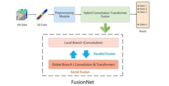
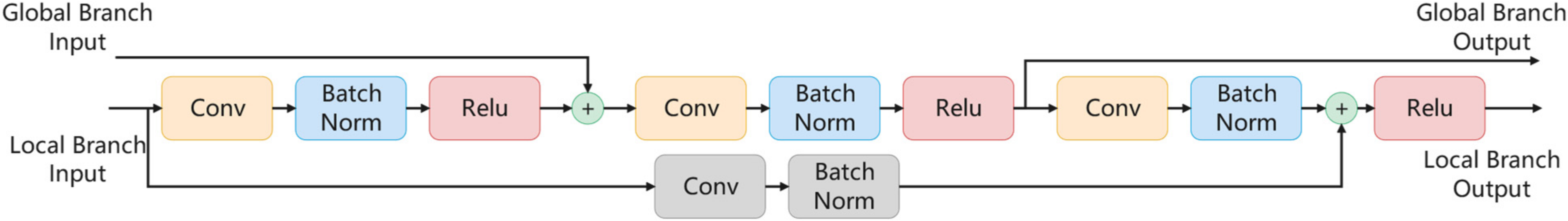
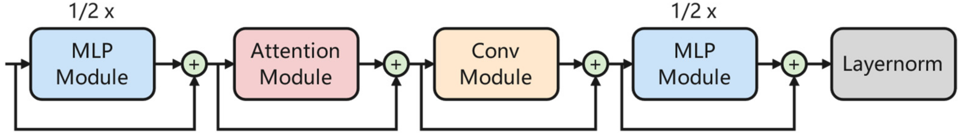
Inspired by the above works, this paper proposes a convolution–Transformer fusion network for HSI classification, known as FusionNet. FusionNet contains two branches, one of which is the Local Branch, consisting of residual-connected convolutional modules and mainly focusing on extracting local information in spatial and spectral dimensions. The other branch is the Global Branch, which is serially connected by Transformer and convolutional modules, and is mainly responsible for extracting global information of spatial and spectral dimensions. The purpose of introducing convolutional modules into this branch is to further enhance the extraction capability of Transformer for local features. In addition, a fusion mechanism is added between the Global Branch and Local branch to enable the communication of local and global information. Hyperspectral images are different from ordinary images, which express a theme as a whole image and possess local features at the spatial–channel level that are more important than hyperspectral images. Thus, CNN is added to Transformer to enhance the ability of the Global Branch to extract local information. The whole network is structured so that the Global Branch and Local Branch are parallel as a whole, while the convolution module and Transformer are serially localized inside the Global Branch. The main contributions of this article are listed as follows:
  • This paper proposes a novel convolution–Transformer fusion network for HSI classification. Considering the strength of convolution in local feature extraction, and the capability of Transformer in long-range contextual relationship extraction, this paper proposes a fusion solution for HSI classification. Local fine-grained features can be well extracted by the convolution module, while global features in the spectral–spatial dimension and long-distance relationships in the spectral dimension can be better extracted by the Transformer module. The fusion of convolution and Transformer successfully enables them to complement each other to achieve better HSI classification results.
  • In FusionNet, a hybrid convolution–Transformer fusion pattern based on serial arrangement and parallel arrangement for a double-branch fusion mechanism was proposed for HSI classification. The Local Branch provides local feature extraction based on convolution, while the Global Branch provides global feature extraction based on convolution–Transformer serial arrangement module. The Local Branch and Global Branch are fused through a double-branch fusion mechanism in a parallel arrangement module. Furthermore, the hybrid fusion pattern enables the fusion and exchange of information between two branches to achieve effective extraction of local and global features.
  • FusionNet achieves competitive results on the three most commonly used datasets. This suggests that the fusion of convolution and Transformer may be a better solution for HSI classification, and provides a reference for further research in the future.
The remainder of the article is organized as follows: Section 2 presents the materials and methods of FusionNet, including the related works and detailed structure of FusionNet. The comparison results of the network on several datasets are given in Section 3. Section 4 presents a discussion of the experimental results and design of FusionNet to further investigate the effectiveness of the structure. Finally, Section 5 summarizes the entire work and the future directions.

2. Materials and Methods

This Section contains a detailed description of the related work and the structure of FusionNet. First, from Section 2.1 to Section 2.4, the classical structures in FusionNet will be introduced, including the attention mechanism, LayerNorm, residual connectivity, etc. Subsequently, Section 2.5 will provide a detailed description of the proposed FusionNet.

2.1. Attention Mechanism

The attention mechanism draws on the human attention mechanism to select the information that is more important to the task from numerous information sources. Three matrices are obtained by three linear computations of the inputs; namely key, query, and value. Key is the key-value matrix. Query refers to the query matrix, and value is the weight matrix. By calculating the similarity of each pair of query and key, the value corresponding to each key is obtained. Finally, the value is weighted and summed to obtain the final output. In Equation (1), let key be K, query be Q, and value be V.
O u t p u t ( Q , K , V ) = s o f t m a x ( Q K T ) V
Q and V are calculated as follows, where W Q , W K , and W V are the parameter matrices to be learned.
Q = I n p u t × W Q
K = I n p u t × W K
V = I n p u t × W V
The self-attention mechanism is one of the attention mechanisms, which reduces the dependence on external data and is better at capturing the internal relevance of data or features. The calculation process of the self-attention mechanism is shown in Figure 1. The scaled dot-product attention mechanism is used in Transformer, which differs from normal self-attention mechanisms in terms of scaling the results of the dot-products of Q and K. As shown below, d k is the input dimension of the key.
O u t p u t ( Q , K , V ) = s o f t m a x Q K T d k V
The multihead self-attention mechanism decomposes the dimensions that the self-attention mechanism needs to learn to extract the correct features more easily. Figure 2 shows the process of the multihead self-attention mechanism. First, Q, K, and V are, respectively, fed into multiple linear layers, then the attention mechanism is performed. Finally, the results obtained from each attention mechanism are concatenated and output through a linear layer.

2.2. LayerNorm

The normalization layer serves to restrict the data to a certain range to facilitate subsequent processing, prevent gradient vanishing and gradient explosion, and speed up network training. The commonly used mechanisms are batch normalization (BatchNorm) [44], layer normalization (LayerNorm) [45], instance normalization (InstanceNorm) [46], group normalization (GroupNorm) [47], etc.; the most commonly used is BatchNorm. LayerNorm normalizes on the hidden layer, i.e., it normalizes all neuronal inputs of a particular layer.
Figure 3 shows the difference between LayerNorm and BatchNorm. LayerNorm and BatchNorm are very similar, while their major difference is the normalization dimension. LayerNorm normalizes from the sample dimension, while BatchNorm normalizes from the feature dimension; therefore, LayerNorm has better performance for sequences of uncertain length compared to BatchNorm.

2.3. Residual Connection and Dense Connection

Usually, the deeper a network is, the better the results. However, gradient vanishing and gradient explosion may occur when the network is very deep due to the nonlinearity of the activation function, making it difficult to improve the accuracy or even decrease the accuracy.
Residual connectivity is a connection method used between modules within the FusionNet, and originated from ResNet [48]. Such a connection structure allows shallow features to reach the deeper layers of the network so that networks with many layers can be trained [49].
The proposal of DenseNet [50] was inspired by ResNet, where the input of each module is a merge of all previous modules, enabling a more efficient transfer of features and gradients and making the network easier to train. Although the Dense Connection network is narrower and has fewer parameters, it brings an increase in the number of channels, making the network too complex and consuming a lot of memory during training. In contrast, the residual connections only add up the values, but the number of channels does not change.

2.4. Bottleneck

Bottleneck is a structure often used in ResNet [48], which uses several small 1 × 1 convolutional kernels to replace part of the work of the large middle convolutional kernel, reducing the number of parameters and reducing the network size significantly while achieving the same effect.
The remaining 3 × 3 convolutional kernels in the middle can also introduce some spatial information, and play a role similar to positional coding.

2.5. Proposed Method

In this section, the detailed structure of FusionNet is introduced. Figure 4 provides an overview of FusionNet. In general, the proposed FusionNet network is divided into four main parts: a preprocessing module, the Local Branch consisting of a residually connected convolution module, the Global Branch consisting of a Transformer module that incorporates convolution operations, i.e., the Convolution–Transformer Block, and a double-branch fusion mechanism. First, a 3D cube containing the center pixel need to be classified and its neighboring pixels is extracted from the original HSI image as the network input. After being processed by the preprocessing module, the data are fed into the Local Branch and Global Branch, respectively, for parallel extraction. The two branches can both process data in parallel and fuse with each other: the double-branch fusion mechanism can fuse the information between two different branches to achieve a better utilization of the local and global spatial spectral information. Finally, the classification results obtained from the two branches are given equal weights, and the obtained probabilities are summed and passed through Softmax. The maximum value obtained is the prediction result.

2.5.1. Preprocessing Module

Figure 5 illustrates the structure of the preprocessing module. HSI data are rich in spectral–spatial information, and the adopted data preprocessing method plays a crucial role in determining whether this information can be effectively mined and utilized. In this paper, the method of extracting the 3D cube from the original HSI data is adopted to obtain the input data of the network. Furthermore, a preprocessing module is designed according to the characteristics of each of the two branches. The preprocessing module will provide the two branches with input data suitable for both branches, in order to achieve better classification results. The Local Branch and Global Branch have their own characteristics regarding the way they utilize data. Especially for the Global Branch, the HSI data that are closer to the image may not be suitable to be directly used as inputs for the Global Branch. In the preprocessing module of FusionNet, different data preprocessing methods are designed for these two networks in such a way that the performance of each branch will be better utilized. First, the input 3D cube passes through a convolutional layer with a kernel size of 7 and a stride size of 2, and a pooling layer with a kernel size of 3 and a stride size of 2, to extract the local features of the data. For the Global Branch, an additional learnable class token is used and spliced with the output data of the pooling layer, and then passed through a transformer encoder module to obtain the input data of the Global Branch [39]; this is similar to the approach the vision Transformer model. Since the convolution module itself incorporates position information into the output, position encoding is no longer needed in the subsequent Transformer encoder module. For the Local Branch, the data from the pooling layer are passed through a three-layer convolution module with a bottleneck structure to obtain the input data for the Local Branch. The detailed structure of the convolution module will be described later.

2.5.2. Local Branch

The Local Branch is mainly composed of two consecutive convolution modules. Figure 6 illustrates the structure of the convolution module in the Local Branch. Inspired by [42], a serial convolution–Transformer connection was designed for HSI images. It is called the Local Branch since the convolution operation is better at capturing local features. The same applies to the other branch. Similar to the bottleneck layer in ResNet, each convolution module contains three layers of convolutional networks, i.e., two convolutional layers with kernel size 1 × 1 and stride 1 at the beginning and end, respectively, and one convolutional layer with kernel size 3 × 3 and stride 1 at the center, using residual connections between the beginning and the end. The bottleneck structure reduces the dimensionality first and then raises it. The bottleneck reduces the number of parameters significantly while ensuring the efficient use of spatial features in HSI data, which enhances the efficiency of network training. In addition, the two convolution modules provide an interface for information interaction with the Global Branch. The output of the first convolution module will be utilized by the Global Branch, further enhancing the ability of the Global Branch to utilize local features; the input of the second convolution module will fuse the intermediate results from the Global Branch, further enhancing the ability of the Local Branch to characterize global features.

2.5.3. Global Branch

The Global Branch mainly consists of a convolution–Transformer module with an additional convolution module and an information interaction interface with the Local Branch. Benefiting from the attention mechanism, the Global Branch possesses a better ability to capture global features. In this module, the convolution–Transformer module and the Transformer module are connected together in a serial manner. Figure 7 illustrates the structure of the convolution–transformer module in the Local Branch. The module consists of four main submodules: MLP module, multihead self-attention module, convolution module, and layer normalization module, each of which is connected by residuals. The Transformer module has a sandwich-like network structure, i.e., the multihead self-attention module and the convolution module are sandwiched between two feedforward modules. The feedforward module mainly consists of two linear layers, and uses Swish as the activation function. The multihead self-attention module mainly consists of a multihead self-attention mechanism with the addition of a relative positional embedding. The convolution module uses depthwise convolution and pointwise convolution, which have lower parameter numbers and operation costs compared with traditional convolution. In addition, the convolution module also uses two activation layers, GLU (gated linear unit) [51] and Swish [52]. Assuming that the input of the convolution–Transformer module is x, and the final output is y, the output of the whole convolution–Transformer module can be shown by the following equation:
x 1 = x 0 + 1 2 M L P ( x 0 )
x 2 = x 1 + M H S A ( x 1 )
x 3 = x 2 + C o n v o l u t i o n ( x 2 )
y = L a y e r n o r m ( x 3 + 1 2 M L P ( x 3 ) )
where MLP stands for MLP module, MHSA stands for multihead self-attention module, Convolution stands for convolution module, and Layernorm stands for layer normalization module.

2.5.4. Double-Branch Fusion Mechanism

The Local Branch has excellent extraction capability for local spatial features, while the Global Branch has the advantage of extracting global spatial and spectral features. Therefore, inspired by [43], the double-branch fusion mechanism is used to help the two branches exchange information so that each branch can take advantage of the other. Figure 8 illustrates the structure of the double-branch fusion mechanism. The double-branch fusion mechanism consists of a down module and an up module. The down module mainly consists of a convolutional layer of kernel size 1, a GELU (Gaussian error linear unit) [53] activation layer, and a mean pooling layer. Layer normalization is added to be responsible for incorporating the information of the Global Branch into the CNN branch. The up module consists of a kernel size of 1, a convolutional layer, a RELU activation layer, and a batch normalization module, and finally interpolates to complete the dimensional alignment with the Global Branch feature map. A convolutional layer of kernel size 1 is introduced to enable cross-channel information interaction and help further exploit the HSI data with rich spectral features. The two-branch fusion mechanism starts from the first convolution module in the Local Branch: the data output from the first convolution module travels through the down module to complete the dimensional alignment with the Global Branch. After that, it is sent to the convolution–Transformer module, together with the original input from the Global Branch. After convolution–Transformer module fusion, data from the Global Branch are returned to the Local Branch through the up module. The fusion mechanism ensures that both branches can recognize the features extracted from the other branch, further improving the network’s ability to utilize local fine-grained features and global contextual relationships.

3. Experiments

In this section, three well-known public hyperspectral image datasets are used. Next, the proposed FusionNet network is applied to these three datasets. The performance of the proposed FusionNet network is validated by comparing it with the prevailing network structures in the field of hyperspectral image classification.

3.1. Dataset Description

In experiments, to validate the classification capability of the proposed FusionNet, three most commonly used public datasets of hyperspectral images were selected for comparison: the Indian Pines dataset, the Pavia University dataset, and the recently available Houston dataset. The basic information regarding the selected datasets is shown in Table 1.
Indian Pines is the earliest test dataset for hyperspectral image classification, imaged by AVIRIS in 1992 on an Indian pine tree in Indiana, USA, with a spatial size of 145 × 145 pixels; the number of remaining spectral channels was 200 and the number of land cover classes was 16, after removing 20 of the bands that were interfered by noise. The detailed land cover categories and the corresponding sample numbers are shown in Table 2.
The false-color map and ground truth map of Indian Pines dataset are shown in Figure 9.
The Pavia University dataset was obtained from the German airborne Reflective Optics Spectrographic Imaging System (ROSIS), taken in 2003 at the University of Pavia in Italy. The spatial size is 610 × 340 pixels. In the classification, 12 bands affected by noise were removed. The number of spectral channels used for the actual classification is 103, and the number of land cover categories is 9. The details of the land cover categories and the corresponding sample numbers are shown in Table 3.
The false-color map and ground truth map of the Pavia University dataset are shown in Figure 10.
The Houston dataset was sourced from the Hyperspectral Image Analysis Group at the University of Houston and the NSF-funded Center for Airborne Laser Mapping (NCALM). It was initially used in the IEEE GRSS data fusion competition in 2013. The spatial size is 349 × 1905 pixels. The dataset has a spatial size of 349 × 1905, with 144 spectral channels, and contains 15 classes. The details of the land cover categories and the corresponding sample numbers are shown in Table 4.
The false-color map and ground truth map of the Houston dataset are shown in Figure 11.

3.2. Experimental Settings

To evaluate the classification performance of the proposed FusionNet network, three widely adopted metrics were used, overall accuracy (OA), average accuracy (AA), and the Kappa coefficient, as the evaluation metrics. OA is the ratio of the number of correct predictions made by the network over all test sets to the overall number. AA is the average of the ratio of the number of correct predictions made in each category to the overall number of that category, and the Kappa coefficient reflects the degree of consistency, and takes values in the range [−1, 1]. The higher the value achieved by the network on these three metrics, the better the classification of the network.
The proposed FusionNet uses AdamW as the optimizer of the network. The learning rate is set to 0.0003, and the number of epochs is set to 50. The spatial size of the HSI cube is set to 15 × 15, and the batch size is set to 16. The experiment uses the Pytorch 1.9.0 deep learning framework, Python 3.7 development language, the Ubuntu 18.04.4 operating system, and NVIDIA GeForce RTX 2080 Ti graphics card to accelerate the training process of the proposed FusionNet network.

3.3. Experimental Results

To demonstrate the effectiveness of the proposed model, several representative models were selected for comparison experiments with the proposed model: the RBF-SVM [10], CDCNN [30], DBMA [54], DBDA [9], SSRN [55], FDSSC [56], DMuCA [28], and SSFTT [41]. RBF-SVM is one of the most classical traditional HSI classification methods; CDCNN, SSRN, and FDSSC are representative convolution-based HSI classification methods; DBMA and DBDA are representative attention mechanism-based HSI classification methods; and DMuCA and SSFTT are recently proposed state-of-the-art HSI classification methods.

3.3.1. Classification Results of the Indian Pines Dataset

In total, 10% of the samples were randomly selected from the Indian Pines dataset as the training set to train the network, 10% as the validation set, and 80% as the test set. The average classification results of the 10 algorithms after 10 independent runs are given in Table 5, where the first 16 rows correspond to the classification results of each class, and the last three rows are the overall OA, AA, and Kappa coefficient, with the highest accuracy for a specific class shown in bold. Figure 12 shows the classification images obtained for the different methods, where Figure 12a indicates ground truth and Figure 12b–h are the results obtained using different classification networks.
From Table 5, it can be seen that the proposed FusionNet achieved the best classification results with OA of 99.30%, AA of 98.65%, and Kappa coefficient of 99.21%. The traditional classification method, i.e., RBF-SVM classification method, achieved the worst results with the lowest OA, AA, and Kappa coefficient metrics among all the networks used for comparison. CDCNN introduced a convolutional neural network and jointly used the local spectral relationships of adjacent individual pixel vectors for classification, thus achieving better classification results compared to RBF-SVM. However, it can be also observed that the CDCNN results are less stable: the standard deviation of its OA is as high as 8.73% in 10 independent runs. The DBMA and DBDA networks introduced an attention mechanism for classification, and thus achieved more satisfactory classification results: the OA of DBMA improved by about 15% compared to the CDCNN. The DBDA results further improved compared to DBMA. The SSRN and FDSSC can effectively use spatial information and spectral features, and possess similar performances to DBMA, achieving OAs of 98.63% and 98.68% respectively, with good performance in the classification of several categories. DMuCA and SSFTT are more novel HSI classification methods. DMuCA captures spectral–spatial context dependencies through deep convolution and contextual attention mechanisms, and achieved 96.62% OA. SSFTT, which includes Transformer encoders in its network structure, achieved 98.67% OA and performed well on several categories. However, compared to all other networks, the proposed FusionNet achieved a superior performance in terms of overall results. Although the classification results of FusionNet are lower than the others in a few classes, FusionNet achieves the best performance in all three metrics, OA, AA, and the Kappa coefficient, revealing the excellent classification ability of FusionNet. Among the classification result images, it is found that the results of RBF-SVM showed the most noise, a large number of misclassified regions, and significantly worse results than the deep-learning-based classification networks. Among these methods, FusionNet exhibited the least noise and hardly any misclassified regions were visible from the classification result images. This corresponds to the results in Table 5.

3.3.2. Classification Results of the Pavia University Dataset

Compared with the Indian Pines dataset, the Pavia University dataset contains a larger amount of data, so it is advisable to use a smaller proportion of the training set to test the performance of FusionNet. In the Pavia University dataset, 5% of the data were randomly selected as the training set to train the network, 5% of the samples were selected as the validation set, and 90% of the samples were selected as the test set. The classification results of different networks on the Pavia University dataset are listed in Table 6, and the highest accuracies for specific categories are shown in bold. The visualization of the results obtained from different networks is shown in Figure 13. As can be seen from Table 6, the SVM still performs poorly in terms of OA, and its classification result images also show a large degree of mislabeling. This is significantly improved in the subsequent networks: DBMA, DBDA, CDCNN, SSRN, FDSSC, DMuCA, and SSFTT. The best classification results can be achieved using the proposed FusionNet network: the classification graph obtained using the proposed FusionNet network performs well on the classification maps, and the classification results are accurate and almost identical to the ground truth. Similarly, the proposed method achieved the best performance in the three metrics of OA, AA, and the Kappa coefficient, reaching 99.92%, 99.63%, and 98.64%, respectively.

3.3.3. Classification Results of the Houston Dataset

The same ratio of dataset partitioning was adopted in the Houston dataset as in the Indian Pines dataset: 10% of the randomly selected feature samples were used as the training set to train the network, 10% as the validation set, and 80% as the test set. The classification results of different networks on the Houston dataset are listed in Table 7, and the highest accuracy for specific categories is shown in bold. The classification plots for the different methods are shown in Figure 14. As can be seen, although the proposed FusionNet network did not achieve the best results in all individual category classification accuracies, the proposed FusionNet network performed well in terms of overall classification results: accurate classification was achieved in the results of almost all categories, with individual category classification accuracies above 98%, and ranked first among all networks with an overall accuracy of 99.28% and an average accuracy of 99.33%.

4. Discussion

The experimental results of FusionNet on three datasets from Indian Pines, Pavia University, and Houston demonstrate the power of the fusion of convolution and Transformer. This chapter will discuss the network structure and experimental results of FusionNet to further demonstrate the effectiveness and possible value of proposed structure for future research.

4.1. Ablation Study

This paper proposed a hybrid convolution–Transformer fusion pattern. The FusionNet structure with convolution operations and Transformer should be arranged in parallel overall and serially arranged locally (i.e., within the Global Branch), helping to further extract features from HSI data and further enhance the effectiveness of HSI classification methods. To prove the proposed point, two comparison models are designed based on the original FusionNet: (a) serial arrangement of convolutional and attention operations, i.e., using only the Convolution–Transformer Block as the core network structure for classifying and keeping the other modules unchanged; (b) parallel arrangement of convolutional and attention operations, i.e., the Convolution–Transformer Block in FusionNet is replaced by a normal Transformer encoder and keeps the other modules unchanged. Table 8 and Table 9 show the comparison of the experimental results of (a), (b), and the original FusionNet for the three datasets. It can be observed that among the three networks, (a), which uses only serial alignment, performed the worst overall on the three datasets, especially when the amount of available training data is limited. For example, on the Indian Pines dataset, (a) achieves an overall accuracy of only 83.09%, which is not far from both (b) and the full FusionNet. In comparison, (b), which uses only parallel alignment, achieved better results relative to (a), but its results still fall short of those of FusionNet. The best results were obtained when fusing serial alignment with parallel alignment, i.e., using FusionNet for classification, with more significant improvements in both individual category classification accuracy, overall accuracy, average accuracy, and the Kappa coefficient, proving the effectiveness of the proposed method.

4.2. Parameter Analysis

4.2.1. Effect of Patch Size on Classification Results

To take full advantage of the spectral–spatial information of HSI, 3D cubes of a certain size around the central pixel were selected from the original data to be input into the network. The size of the 3D cubes selected in this way directly affects the amount of information used for classification and, to some extent, the classification accuracy. To evaluate the effect of the size of the cube on the classification results, the effect on the training results was explored by continuously increasing the patch size, i.e., by increasing the size of the cube in the spatial dimension. In this analysis, DMuCA, SSFTT, SSRN, FDSSC, DBMA, DBDA, and the proposed method were selected for comparison. The patch size is set to 5, 7, 9, 11, 13, 15, and 17, respectively, and the results obtained with the Indian Pines dataset are shown in Figure 15.
From Figure 15, it can be seen that increasing the patch size will introduce more spectral–spatial information, which contributes to the classification accuracy. However, a larger patch size does not necessarily lead to better results. Larger patch size will bring higher computational cost and may also introduce more irrelevant information, thus causing a loss of accuracy. It can be seen that for a given different patch size, FusionNet is consistently able to exhibit high classification accuracy, reflecting good spectral–spatial information utilization. For FusionNet, it can be found that when the patch size is between 5 and 7, the overall accuracy, average accuracy, and kappa indicators all increase significantly with the increase in the spatial dimension input size. Additionally, when the patch size is between 7 and 11, the classification result indicators increase slowly, and when the patch size is larger than 11, the classification results no longer continue to grow with the increase in patch size. Considering the performance and cost, a patch size of 7 was chosen as the parameter used in the experiments, i.e., the size of the HSI cube is 15 × 15 in the spatial dimension.

4.2.2. Effect of Training Set Size on Classification Results

In practice, accurate manual labeling of pixels in large amounts of HSI data is relatively difficult, thus, the number of labeled samples available for training HSI networks may not be sufficient. Therefore, the proposed classification network should demonstrate good classification results under different training set sizes. To analyze the performance of the proposed FusionNet with different training set sizes, FusionNet was tested against the Indian Pines dataset, and was compared with other models, namely RBF-SVM, CDCNN, DBMA, DBDA, SSRN, FDSSC, DMuCA, and SSFTT. All models were tested using training set proportions of 3%, 5%, 10%, 15%, and 20%, respectively, and the results obtained are shown in Figure 16. From the results, it can be seen that the classification results achieved by FusionNet improve significantly as the proportion of the training set increases. It is also observed that FusionNet, SSFTT, FDSSC, and DBDA achieved good classification results with a small percentage of the training set (3%). Meanwhile, FusionNet still achieved competitive classification results compared to other models, i.e., an OA of 93.36%. When the training set percentage reached 10%, the OA of FusionNet had already reached 99.30%. The experimental results show that FusionNet has good adaptability to different training set sizes.

5. Conclusions

In this paper, the FusionNet and a two-branch convolution–Transformer fusion network for HSI classification, and innovatively designed parallel and serial convolution–Transformer fusion methods are proposed. The proposed network has two branches, the Local Branch that focuses on local information extraction in spatial and spectral dimensions, and the Global Branch, which is responsible for extracting global information. Subsequently, the features of the two branches are fused to form spatial–spectral features for the final classification results. Overall, the convolution and Transformer modules are fused in parallel, while the convolution and Transformer modules are serially arranged to further enhance the extraction capability of the local features within the Global Branch. Experimental results for three genuine HSI datasets show that the proposed FusionNet network exhibits excellent classification results with a significant advantage over previous works, especially when the labeled training data are very limited. This work provides an optimization scheme for the processing and analysis of HSI classification. Future research will focus on optimizing the network structure to further improve the classification accuracy and further reduce the dependence on the amount of training data.

Author Contributions

Investigation, L.Y., Y.Y. and J.Y.; Methodology, L.Y., Y.Y., N.Z. and J.Y.; Writing, L.Y. and Y.Y.; Editing, J.Y., T.W. and L.W. (Ling Wu); Valuable advice, L.W. (Liguo Wang). All authors have read and agreed to the published version of the manuscript.

Funding

This research was funded by the National Natural Science Foundation of China (Nos. 62001434, 62071084).

Data Availability Statement

Publicly available datasets were analyzed in this study, which can be found here: http://www.ehu.eus/ccwintco/index.php/Hyperspectral_Remote_Sensing_Scenes (accessed on 16 March 2022) and https://hyperspectral.ee.uh.edu/?page_id=459 (accessed on 17 March 2022).

Acknowledgments

The authors would like to thank the authors of all references used in the paper, the editors, and the anonymous reviewers for their detailed comments and suggestions.

Conflicts of Interest

The authors declare no conflict of interest.

References

  1. Landgrebe, D. Hyperspectral image data analysis. IEEE Signal Process. Mag. 2002, 19, 17–28. [Google Scholar] [CrossRef]
  2. Ahmed, N.; Khan, S.H.; Anjum, M.A.; Rehman, A. A cost effective preparative thin layer chromatography cleanup method for high performance liquid chromatography analysis of aflatoxins B1, B2 and G2. Adv. Life Sci. 2014, 2, 1–4. [Google Scholar]
  3. Pipitone, C.; Maltese, A.; Dardanelli, G.; Lo Brutto, M.; La Loggia, G. Monitoring water surface and level of a reservoir using different remote sensing approaches and comparison with dam displacements evaluated via GNSS. Remote Sens. 2018, 10, 71. [Google Scholar] [CrossRef] [Green Version]
  4. Awad, M.; Jomaa, I.; Arab, F. Improved capability in stone pine forest mapping and management in Lebanon using hyperspectral CHRIS-Proba data relative to Landsat ETM+. Photogramm. Eng. Remote Sens. 2014, 80, 725–731. [Google Scholar] [CrossRef]
  5. Luo, B.; Yang, C.; Chanussot, J.; Zhang, L. Crop yield estimation based on unsupervised linear unmixing of multidate hyperspectral imagery. IEEE Trans. Geosci. Remote Sens. 2012, 51, 162–173. [Google Scholar] [CrossRef]
  6. Bishop, C.A.; Liu, J.G.; Mason, P.J. Hyperspectral remote sensing for mineral exploration in Pulang, Yunnan Province, China. Int. J. Remote Sens. 2011, 32, 2409–2426. [Google Scholar] [CrossRef]
  7. Bhatt, J.S.; Joshi, M.V. Deep learning in hyperspectral unmixing: A review. In Proceedings of the IGARSS 2020—2020 IEEE International Geoscience and Remote Sensing Symposium, Waikoloa, HI, USA, 26 September–2 October 2020; pp. 2189–2192. [Google Scholar]
  8. Zhao, X.; Li, W.; Shan, T.; Li, L.; Tao, R. Hyperspectral target detection by fractional Fourier transform. In Proceedings of the IGARSS 2020—2020 IEEE International Geoscience and Remote Sensing Symposium, Waikoloa, HI, USA, 26 September–2 October 2020; pp. 1655–1658. [Google Scholar]
  9. Li, R.; Zheng, S.; Duan, C.; Yang, Y.; Wang, X. Classification of hyperspectral image based on double-branch dual-attention mechanism network. Remote Sens. 2020, 12, 582. [Google Scholar] [CrossRef] [Green Version]
  10. Melgani, F.; Bruzzone, L. Classification of hyperspectral remote sensing images with support vector machines. IEEE Trans. Geosci. Remote Sens. 2004, 42, 1778–1790. [Google Scholar] [CrossRef] [Green Version]
  11. Aswathy, C.; Sowmya, V.; Gandhiraj, R.; Soman, K. Hyperspectral image denoising using legendre Fenchel Transformation for improved Multinomial Logistic Regression based classification. In Proceedings of the 2015 International Conference on Communications and Signal Processing (ICCSP), Melmaruvathur, India, 2–4 April 2015; pp. 1670–1674. [Google Scholar]
  12. Belgiu, M.; Drăguţ, L. Random forest in remote sensing: A review of applications and future directions. ISPRS J. Photogramm. Remote Sens. 2016, 114, 24–31. [Google Scholar] [CrossRef]
  13. Chen, Y.; Nasrabadi, N.M.; Tran, T.D. Hyperspectral image classification via kernel sparse representation. IEEE Trans. Geosci. Remote Sens. 2012, 51, 217–231. [Google Scholar] [CrossRef] [Green Version]
  14. Tarabalka, Y.; Chanussot, J.; Benediktsson, J.A. Segmentation and classification of hyperspectral images using watershed transformation. Pattern Recognit. 2010, 43, 2367–2379. [Google Scholar] [CrossRef] [Green Version]
  15. Chen, Y.; Nasrabadi, N.M.; Tran, T.D. Hyperspectral image classification using dictionary-based sparse representation. IEEE Trans. Geosci. Remote Sens. 2011, 49, 3973–3985. [Google Scholar] [CrossRef]
  16. Ahmad, M.; Shabbir, S.; Roy, S.K.; Hong, D.; Wu, X.; Yao, J.; Khan, A.M.; Mazzara, M.; Distefano, S.; Chanussot, J. Hyperspectral image classification—Traditional to deep models: A survey for future prospects. IEEE J. Sel. Top. Appl. Earth Obs. Remote Sens. 2021, 15, 968–999. [Google Scholar] [CrossRef]
  17. Li, S.; Song, W.; Fang, L.; Chen, Y.; Ghamisi, P.; Benediktsson, J.A. Deep learning for hyperspectral image classification: An overview. IEEE Trans. Geosci. Remote Sens. 2019, 57, 6690–6709. [Google Scholar] [CrossRef] [Green Version]
  18. Voulodimos, A.; Doulamis, N.; Doulamis, A.; Protopapadakis, E. Deep learning for computer vision: A brief review. Comput. Intell. Neurosci. 2018, 2018, 7068349. [Google Scholar] [CrossRef]
  19. Otter, D.W.; Medina, J.R.; Kalita, J.K. A survey of the usages of deep learning for natural language processing. IEEE Trans. Neural Netw. Learn. Syst. 2020, 32, 604–624. [Google Scholar] [CrossRef] [Green Version]
  20. Sun, L.; Cheng, S.; Zheng, Y.; Wu, Z.; Zhang, J. SPANet: Successive Pooling Attention Network for Semantic Segmentation of Remote Sensing Images. IEEE J. Sel. Top. Appl. Earth Obs. Remote Sens. 2022, 15, 4045–4057. [Google Scholar] [CrossRef]
  21. Wang, J.; Song, X.; Sun, L.; Huang, W.; Wang, J. A novel cubic convolutional neural network for hyperspectral image classification. IEEE J. Sel. Top. Appl. Earth Obs. Remote Sens. 2020, 13, 4133–4148. [Google Scholar] [CrossRef]
  22. Chen, Y.; Lin, Z.; Zhao, X.; Wang, G.; Gu, Y. Deep learning-based classification of hyperspectral data. IEEE J. Sel. Top. Appl. Earth Obs. Remote Sens. 2014, 7, 2094–2107. [Google Scholar] [CrossRef]
  23. Hu, W.; Huang, Y.; Wei, L.; Zhang, F.; Li, H. Deep Convolutional Neural Networks for Hyperspectral Image Classification. J. Sens. 2015, 2015, 258–619. [Google Scholar] [CrossRef] [Green Version]
  24. Mou, L.; Ghamisi, P.; Zhu, X.X. Deep recurrent neural networks for hyperspectral image classification. IEEE Trans. Geosci. Remote Sens. 2017, 55, 3639–3655. [Google Scholar] [CrossRef] [Green Version]
  25. Zhu, L.; Chen, Y.; Ghamisi, P.; Benediktsson, J.A. Generative adversarial networks for hyperspectral image classification. IEEE Trans. Geosci. Remote Sens. 2018, 56, 5046–5063. [Google Scholar] [CrossRef]
  26. Mou, L.; Lu, X.; Li, X.; Zhu, X.X. Nonlocal graph convolutional networks for hyperspectral image classification. IEEE Trans. Geosci. Remote Sens. 2020, 58, 8246–8257. [Google Scholar] [CrossRef]
  27. Jiang, Y.; Li, Y.; Zou, S.; Zhang, H.; Bai, Y. Hyperspectral image classification with spatial consistence using fully convolutional spatial propagation network. IEEE Trans. Geosci. Remote Sens. 2021, 59, 10425–10437. [Google Scholar] [CrossRef]
  28. Liang, M.; He, Q.; Yu, X.; Wang, H.; Meng, Z.; Jiao, L. A Dual Multi-Head Contextual Attention Network for Hyperspectral Image Classification. Remote Sens. 2022, 14, 3091. [Google Scholar] [CrossRef]
  29. Yue, J.; Zhao, W.; Mao, S.; Liu, H. Spectral–spatial classification of hyperspectral images using deep convolutional neural networks. Remote Sens. Lett. 2015, 6, 468–477. [Google Scholar] [CrossRef]
  30. Lee, H.; Kwon, H. Going deeper with contextual CNN for hyperspectral image classification. IEEE Trans. Image Process. 2017, 26, 4843–4855. [Google Scholar] [CrossRef] [Green Version]
  31. Roy, S.K.; Krishna, G.; Dubey, S.R.; Chaudhuri, B.B. HybridSN: Exploring 3-D–2-D CNN feature hierarchy for hyperspectral image classification. IEEE Geosci. Remote Sens. Lett. 2019, 17, 277–281. [Google Scholar] [CrossRef] [Green Version]
  32. Chang, Y.-L.; Tan, T.-H.; Lee, W.-H.; Chang, L.; Chen, Y.-N.; Fan, K.-C.; Alkhaleefah, M. Consolidated Convolutional Neural Network for Hyperspectral Image Classification. Remote Sens. 2022, 14, 1571. [Google Scholar] [CrossRef]
  33. Meng, Z.; Jiao, L.; Liang, M.; Zhao, F. A lightweight spectral-spatial convolution module for hyperspectral image classification. IEEE Geosci. Remote Sens. Lett. 2021, 19, 1–5. [Google Scholar] [CrossRef]
  34. He, X.; Chen, Y.; Lin, Z. Spatial-spectral transformer for hyperspectral image classification. Remote Sens. 2021, 13, 498. [Google Scholar] [CrossRef]
  35. Hong, D.; Han, Z.; Yao, J.; Gao, L.; Zhang, B.; Plaza, A.; Chanussot, J. SpectralFormer: Rethinking hyperspectral image classification with transformers. IEEE Trans. Geosci. Remote Sens. 2021, 60, 1–15. [Google Scholar] [CrossRef]
  36. Xu, Y.; Du, B.; Zhang, L. Self-attention context network: Addressing the threat of adversarial attacks for hyperspectral image classification. IEEE Trans. Image Process. 2021, 30, 8671–8685. [Google Scholar] [CrossRef]
  37. Fang, B.; Li, Y.; Zhang, H.; Chan, J.C.-W. Hyperspectral images classification based on dense convolutional networks with spectral-wise attention mechanism. Remote Sens. 2019, 11, 159. [Google Scholar] [CrossRef] [Green Version]
  38. Vaswani, A.; Shazeer, N.; Parmar, N.; Uszkoreit, J.; Jones, L.; Gomez, A.N.; Kaiser, Ł.; Polosukhin, I. Attention is all you need. arXiv 2017, arXiv:1706.03762. [Google Scholar]
  39. Dosovitskiy, A.; Beyer, L.; Kolesnikov, A.; Weissenborn, D.; Zhai, X.; Unterthiner, T.; Dehghani, M.; Minderer, M.; Heigold, G.; Gelly, S. An image is worth 16x16 words: Transformers for image recognition at scale. arXiv 2020, arXiv:2010.11929. [Google Scholar]
  40. Liu, B.; Yu, A.; Gao, K.; Tan, X.; Sun, Y.; Yu, X. DSS-TRM: Deep spatial–spectral transformer for hyperspectral image classification. Eur. J. Remote Sens. 2022, 55, 103–114. [Google Scholar] [CrossRef]
  41. Sun, L.; Zhao, G.; Zheng, Y.; Wu, Z. Spectral–Spatial Feature Tokenization Transformer for Hyperspectral Image Classification. IEEE Trans. Geosci. Remote Sens. 2022, 60, 1–14. [Google Scholar] [CrossRef]
  42. Gulati, A.; Qin, J.; Chiu, C.-C.; Parmar, N.; Zhang, Y.; Yu, J.; Han, W.; Wang, S.; Zhang, Z.; Wu, Y. Conformer: Convolution-augmented transformer for speech recognition. arXiv 2020, arXiv:2005.08100. [Google Scholar]
  43. Peng, Z.; Huang, W.; Gu, S.; Xie, L.; Wang, Y.; Jiao, J.; Ye, Q. Conformer: Local Features Coupling Global Representations for Visual Recognition. In Proceedings of the IEEE/CVF International Conference on Computer Vision, Montreal, QC, Canada, 10–17 October 2021; pp. 367–376. [Google Scholar]
  44. Ioffe, S.; Szegedy, C. Batch normalization: Accelerating deep network training by reducing internal covariate shift. Proc. Mach. Learn. Res. 2015, 37, 448–456. [Google Scholar]
  45. Ba, J.L.; Kiros, J.R.; Hinton, G.E. Layer normalization. arXiv 2016, arXiv:1607.06450. [Google Scholar]
  46. Ulyanov, D.; Vedaldi, A.; Lempitsky, V. Instance normalization: The missing ingredient for fast stylization. arXiv 2016, arXiv:1607.08022. [Google Scholar]
  47. Wu, Y.; He, K. Group normalization. In Proceedings of the European Conference on Computer Vision (ECCV) 15th European Conference, Munich, Germany, 8–14 September 2018; pp. 3–19. [Google Scholar]
  48. He, K.; Zhang, X.; Ren, S.; Sun, J. Deep residual learning for image recognition. In Proceedings of the IEEE Conference on Computer Vision and Pattern Recognition, Las Vegas, NV, USA, 27–30 June 2016; pp. 770–778. [Google Scholar]
  49. Srivastava, R.K.; Greff, K.; Schmidhuber, J. Highway networks. arXiv 2015, arXiv:1505.00387. [Google Scholar]
  50. Huang, G.; Liu, Z.; Van Der Maaten, L.; Weinberger, K.Q. Densely connected convolutional networks. In Proceedings of the IEEE Conference on Computer Vision and Pattern Recognition, Honolulu, HI, USA, 21–26 July 2017; pp. 4700–4708. [Google Scholar]
  51. Dauphin, Y.N.; Fan, A.; Auli, M.; Grangier, D. Language modeling with gated convolutional networks. Proc. Mach. Learn. Res. 2017, 70, 933–941. [Google Scholar]
  52. Ramachandran, P.; Zoph, B.; Le, Q.V. Searching for activation functions. arXiv 2017, arXiv:1710.05941. [Google Scholar]
  53. Hendrycks, D.; Gimpel, K. Gaussian error linear units (gelus). arXiv 2016, arXiv:1606.08415. [Google Scholar]
  54. Ma, W.; Yang, Q.; Wu, Y.; Zhao, W.; Zhang, X. Double-branch multi-attention mechanism network for hyperspectral image classification. Remote Sens. 2019, 11, 1307. [Google Scholar] [CrossRef] [Green Version]
  55. Zhong, Z.; Li, J.; Luo, Z.; Chapman, M. Spectral–spatial residual network for hyperspectral image classification: A 3-D deep learning framework. IEEE Trans. Geosci. Remote Sens. 2017, 56, 847–858. [Google Scholar] [CrossRef]
  56. Wang, W.; Dou, S.; Jiang, Z.; Sun, L. A fast dense spectral–spatial convolution network framework for hyperspectral images classification. Remote Sens. 2018, 10, 1068. [Google Scholar] [CrossRef] [Green Version]
Figure 1. Attention mechanism.
Remotesensing 14 04066 g001
Figure 2. The multihead self-attention mechanism.
Remotesensing 14 04066 g002
Figure 3. LayerNorm and BatchNorm.
Remotesensing 14 04066 g003
Figure 4. Overall structure of the proposed FusionNet model.
Remotesensing 14 04066 g004
Figure 5. Preprocessing module.
Remotesensing 14 04066 g005
Figure 6. Convolution module in the Local Branch.
Remotesensing 14 04066 g006
Figure 7. Convolution–Transformer module in the Local Branch.
Remotesensing 14 04066 g007
Figure 8. Double-Branch fusion mechanism.
Remotesensing 14 04066 g008
Figure 9. Indian Pines dataset: (a) false-color map, (b) ground truth map.
Remotesensing 14 04066 g009
Figure 10. Pavia University dataset: (a) false-color map, (b) ground truth map.
Remotesensing 14 04066 g010
Figure 11. Houston dataset: (a) false-color map, (b) ground truth map.
Remotesensing 14 04066 g011
Figure 12. Classification maps of the Indian Pines dataset with 10% training samples.
Remotesensing 14 04066 g012
Figure 13. Classification maps of the Pavia University dataset with 5% training samples.
Remotesensing 14 04066 g013
Figure 14. Classification maps of the Houston dataset with 10% training samples.
Remotesensing 14 04066 g014
Figure 15. Effect of patch size on classification results.
Remotesensing 14 04066 g015
Figure 16. Effect of training set size on classification results.
Remotesensing 14 04066 g016
Table 1. Basic information of each HSI dataset.
DatasetSpatial SizeSpectral SizeNumber of
Classes
Labeled Samples
Indian Pines145 × 1452001610,249
Pavia University610 × 340103942,776
Houston349 × 19051441515,029
Table 2. Ground truth classes and samples of the Indian Pines dataset.
OrderClassLabeled Samples
1Alfalfa46
2Corn-notill1428
3Corn-mintill830
4Corn237
5Grass-pasture483
6Grass-trees730
7Grass-pasture-mowed28
8Hay-windrowed478
9Oats20
10Soybean-notill972
11Soybean-mintill2455
12Soybean-clean593
13Wheat205
14Woods1265
15Buildings-Grass-Trees-Drives386
16Stone-Steel-Towers93
Table 3. Ground truth classes and samples of the Pavia University dataset.
OrderClassLabeled Samples
1Asphalt6631
2Meadows18,649
3Gravel2099
4Trees3064
5Sheets1345
6Bare Soil5029
7Bitumen1330
8Bricks3682
9Shadows947
Table 4. Ground truth classes and samples of the Houston dataset.
OrderClassLabeled Samples
1Healthy grass1251
2Stressed grass1254
3Synthetic grass697
4Trees1244
5Soil1242
6Water325
7Residential1268
8Commercial1244
9Road1252
10Highway1227
11Railway1235
12Parking Lot 11233
13Parking Lot 2469
14Tennis Court428
15Running Track660
Table 5. Classification results of the Indian Pines dataset using 10% training samples.
ClassRBF-SVMDBMADBDACDCNNSSRNFDSSCDMuCASSFTTProposed
155.0758.5394.8298.3793.4297.3387.80100.0097.63
271.3480.8897.1398.7397.9499.0994.3995.9599.14
375.5373.4898.6099.0399.1399.2296.5298.3999.49
461.1872.9597.5099.2498.3298.3883.8999.5399.54
588.7695.3797.4098.7399.2899.0598.1699.7797.05
689.1694.3298.7499.3899.8099.4199.5499.8499.27
785.0560.3384.6594.5294.9098.3792.97100.0096.60
890.3291.4699.39100.00100.00100.00100.00100.0099.95
971.1479.9493.5297.2598.8990.9486.2794.4497.69
1075.7474.9396.0497.6597.2396.9697.9499.4299.71
1177.9784.1197.1499.1798.7798.3599.5099.1999.68
1273.2461.3293.9898.9398.4499.2494.5796.8297.69
1390.8096.2498.8399.6499.8299.0994.59100.0099.74
1491.7493.3798.7899.3899.3699.2299.29100.0099.96
1574.4181.9093.9898.1798.3898.3792.3598.5699.65
1698.1697.0096.0292.9794.0796.3197.9888.1095.53
OA (%)80.0181.7697.1098.8798.6398.6896.6298.6799.30
AA (%)79.3581.0196.0398.2097.9898.0894.7498.1398.65
Kappa (%)77.0979.2796.6998.7198.4498.4996.2998.4899.21
Table 6. Classification results of the Pavia University dataset using 5% training samples.
ClassRBF-SVMCDCNNDBMADBDASSRNFDSSCDMuCASSFTTProposed
193.1798.7799.8195.0699.9199.8799.9299.9299.78
295.4399.7299.9098.5899.9299.9599.9599.9999.65
383.8198.0199.1984.8698.2599.2399.0398.3499.71
496.4298.6099.2697.1799.9399.8199.4799.4299.62
598.6999.5799.6499.92100.0099.94100.0099.6999.88
692.1099.9599.9096.1499.6199.9599.81100.0099.76
786.7199.8899.9694.7499.8899.9199.75100.0099.66
884.5897.6994.3591.6497.2598.0999.3599.2399.75
999.9998.0898.5998.5199.9899.2899.4797.78100.00
OA (%)93.2099.2199.2496.0999.5799.7199.7899.7399.92
AA (%)92.3298.9298.9695.1899.4199.5699.6499.3799.76
Kappa (%)90.9498.9598.9994.8299.4399.6299.8599.6598.64
Table 7. Classification results of the Houston dataset using 10% training samples.
ClassRBF-SVMCDCNNDBMADBDASSRNFDSSCDMuCASSFTTProposed
197.3890.9497.3898.9898.5199.5497.2398.4999.27
298.2695.1398.9199.9199.8299.5798.4499.9199.63
399.5698.7299.89100.00100.00100.0099.88100.0099.66
499.0397.7499.1399.7599.5299.7799.2599.1199.29
597.1599.1199.5399.4699.4099.74100.00100.0099.68
699.7999.1299.89100.00100.00100.0095.66100.0099.60
791.8389.8897.7098.9099.3297.4598.8494.2299.13
887.3694.6698.9999.6099.5498.6198.4097.3299.69
987.5390.6696.8997.8098.6298.5696.4099.2998.44
1092.4584.5897.9398.5898.4198.8097.40100.0098.59
1190.9586.2098.5998.8599.2699.0097.87100.0099.57
1288.0389.7197.4899.1398.8599.3996.1699.6499.33
1381.8694.6898.2898.0999.4197.9899.1298.1099.07
1497.9997.1998.6599.13100.0099.13100.00100.00100.00
1599.3297.4998.8699.0299.3899.2599.92100.0099.02
OA (%)93.6092.4298.3699.1199.2299.0498.2198.9499.28
AA (%)93.9093.7298.5499.1599.3399.1298.3099.0799.33
Kappa (%)93.0891.8198.2299.0499.1598.9698.4898.8599.23
Table 8. Comparison results of (a), (b), and the original FusionNet on the Indian Pines dataset.
Class(a)(b)FusionNet
177.54 ± 10.7193.20 ± 12.2097.63 ± 3.40
283.13 ± 3.7493.74 ± 2.7499.14 ± 0.23
380.97 ± 5.5795.35 ± 1.6599.49 ± 0.29
479.03 ± 4.7196.43 ± 3.4499.54 ± 0.28
586.49 ± 2.9499.24 ± 0.8997.95 ± 1.16
686.33 ± 3.9298.83 ± 0.8899.27 ± 0.46
776.84 ± 22.2490.24 ± 13.5496.60 ± 2.23
891.82 ± 4.0798.27 ± 1.3399.95 ± 0.10
989.14 ± 12.4195.55 ± 8.8897.69 ± 3.53
1082.93 ± 2.0594.14 ± 1.4999.71 ± 0.14
1181.00 ± 9.6296.50 ± 1.0799.68 ± 0.27
1274.51 ± 5.1190.71 ± 2.3297.69 ± 0.85
1390.44 ± 4.1399.75 ± 0.4899.74 ± 0.42
1491.95 ± 5.1097.35 ± 1.3099.96 ± 0.07
1576.65 ± 4.9994.48 ± 2.2799.65 ± 0.43
1694.68 ± 4.7896.86 ± 1.7995.53 ± 2.83
OA (%)83.09 ± 4.7295.85 ± 0.4799.30 ± 0.20
AA (%)83.96 ± 2.5995.67 ± 1.2398.65 ± 0.57
Kappa (%)80.56 ± 5.6395.27 ± 0.5499.21 ± 0.22
Table 9. Comparison results of (a), (b), and the original FusionNet on the Pavia University dataset.
Class(a)(a)FusionNet
187.04 ± 7.6696.03 ± 1.0199.78 ± 0.10
297.21 ± 0.5398.93 ± 0.3499.65 ± 0.22
357.81 ± 35.1994.18 ± 1.9999.71 ± 0.13
498.38 ± 1.5399.04 ± 0.6999.62 ± 0.21
599.63 ± 0.3599.90 ± 0.1099.88 ± 0.04
682.27 ± 15.7597.27 ± 0.7299.76 ± 0.21
753.67 ± 43.8693.64 ± 1.9599.66 ± 0.22
880.63 ± 14.5392.82 ± 0.9699.75 ± 0.30
996.61 ± 5.4696.03 ± 1.01100.00 ± 0.00
OA (%)89.40 ± 7.2597.41 ± 0.1899.92 ± 0.13
AA (%)83.70 ± 13.0596.84 ± 0.4099.63 ± 0.27
Kappa (%)86.14 ± 9.3396.57 ± 0.2498.64 ± 1.16
Publisher’s Note: MDPI stays neutral with regard to jurisdictional claims in published maps and institutional affiliations.

