Article

End-to-End Neural Interpolation of Satellite-Derived Sea Surface Suspended Sediment Concentrations

by
Jean-Marie Vient
1,2,*,
Ronan Fablet
2,
Frédéric Jourdin
3 and
Christophe Delacourt
1
1
UBO, Technopôle Brest-Iroise, 29238 Brest, France
2
IMT-Atlantique Bretagne-Pays de la Loire, Technopôle Brest-Iroise, 29238 Brest, France
3
Service Hydrographique et Océanographique de la Marine (SHOM), 29603 Brest, France
*
Author to whom correspondence should be addressed.
Remote Sens. 2022, 14(16), 4024; https://doi.org/10.3390/rs14164024
Submission received: 13 July 2022 / Revised: 12 August 2022 / Accepted: 15 August 2022 / Published: 18 August 2022
(This article belongs to the Special Issue AI for Marine, Ocean and Climate Change Monitoring)

Abstract

:
The characterization of suspended sediment dynamics in the coastal ocean provides key information for both scientific studies and operational challenges regarding, among others, turbidity, water transparency and the development of micro-organisms using photosynthesis, which is critical to primary production. Due to the complex interplay between natural and anthropogenic forcings, the understanding and monitoring of the dynamics of suspended sediments remain highly challenging. Numerical models still lack the capabilities to account for the variability depicted by in situ and satellite-derived datasets. Through the ever increasing availability of both in situ and satellite-derived observation data, data-driven schemes have naturally become relevant approaches to complement model-driven ones. Our previous work has stressed this potential within an observing system simulation experiment. Here, we further explore their application to the interpolation of sea surface sediment concentration fields from real gappy satellite-derived observation datasets. We demonstrate that end-to-end deep learning schemes—namely 4DVarNet, which relies on variational data assimilation formulation—apply to the considered real dataset where the training phase cannot rely on gap-free references but only on the available gappy data. 4DVarNet significantly outperforms other data-driven schemes such as optimal interpolation and DINEOF with a relative gain greater than 20% in terms of RMSLE and improves the high spatial resolution of patterns in the reconstruction process. Interestingly, 4DVarNet also shows a better agreement between the interpolation performance assessed for an OSSE and for real data. This result emphasizes the relevance of OSSE settings for future development calibration phases before the applications to real datasets.

1. Introduction

Marine sediment fluxes result from a combination of natural and anthropogenic forcing factors [1,2]. The main source of sediment load comes from land, and the resuspension of sediments occurs under the effect of waves, tides and the oceanic general circulation, but also from fish trawling and maritime development, such as harbor sediment dredging and dumping, aggregate extraction, submarine cable installation, offshore wind farm exploitation, oil and gas activities, etc. [3]. Besides these latter anthropogenic stresses, additional ones are expected in the foreseeable future through climate change, involving sea-level and waves’ rise, modifying the remobilization and transport in the coastal zone and the sediment inputs from the continent by the modification in the drainage basins hydraulic regime due to modified rainfall [4].
Tracking suspended particles in shelf seas is of interest for coastal management and marine ecosystem monitoring. Yet, the assessment of sediment fluxes, especially near the bottom of the ocean, is a key issue in the investigation of coastal morphological evolution, habitat changes and pollutant dispersion and behavior [5,6,7]. As the turbidity induced by fine sediment suspensions, especially near the surface of the ocean, impacts the primary production by narrowing the thickness of the euphotic zone [8], the quantification of the suspended sediment concentrations and fluxes, at the scale of the continental shelf, is also a critical aspect to fulfill the boundary conditions of their fine mesh-grid coastal hydrodynamic models [9] used for impact studies. However the quantification of suspended sediment fluxes is generally a difficult task due to the complexity of the hydrodynamic and morpho-dynamic processes in play. In absolute terms, assessing the overall sediment dynamics requires understanding of transport processes of mineral particles in the water column as well as their behavior in the seabed, with resuspension capacities and consolidation within the sediment, oftentimes under the influence of biota, impacting flocculation processes in the water column and the biochemical behavior in the sediment [10].
In this context, deterministic (physics-based) numerical models are usually computationally intensive and inaccurate when assessing sediment fluxes from their continental source to the shelf edge [11,12]. Data-driven methods have emerged as appealing approaches to benefit the available datasets coming from observations and model simulations [13,14,15,16]. Recent advances especially bridge data assimilation formulation and machine learning paradigms [17,18]. These schemes are particularly relevant to addressing the irregular space–time sampling of satellite-derived sea surface dynamics. Following our previous study within an OSSE (Observing System Simulation Experiment) setting [19], we aim at evaluating whether such learning-based schemes apply to real satellite-derived datasets. Then, in this article, in the same way we designed real data experiments. They are typically called OSE (Observing System Experiment). Our contribution is two-fold: (i) we develop a novel application of 4DVarNet schemes [18] for satellite-derived sea surface suspended sediment concentrations (SSSC); (ii) we propose an evaluation framework based on real MODIS satellite image series to benchmark data-driven and learning-based schemes for the reconstruction of satellite-derived SSSC fields. We further assess how OSSE benchmarking experiments based on hydrosedimentary numerical simulations [20] inform performance metrics for real datasets in the OSE experiments.
The remainder is organized as follows. Section 2 details the considered datasets. Section 3 details the processes defined to interpolate observation data, which are the Optimal Interpolation and the new 4DVarNet scheme. Section 4 shows the global and specific performance for each method. And finally Section 5 compares OSSE and OSE configurations and characterizes the limits of the 4DVarNet interpolator.

2. Data

The area of study, presented in the first subsection, is located in the Bay of Biscay. The main geophysical parameter of study is the sea surface suspended sediment concentration (SSSC), which relates to the sediment dynamics. Two sets of SSSC data were used. We present the datasets considered in this study, namely numerical simulation data (Section 2.2) and real satellite-derived MODIS data (Section 2.3). These two sets of data have been used to perform two different kind of experiments carried out in parallel: the simulated data are dedicated to OSSE (Observing System Simulation Experiment) while the real data are dedicated to OSE (Observing System Experiment). Later, Section 4 and Section 5 will compare the results obtained by these two different kinds of experiments.

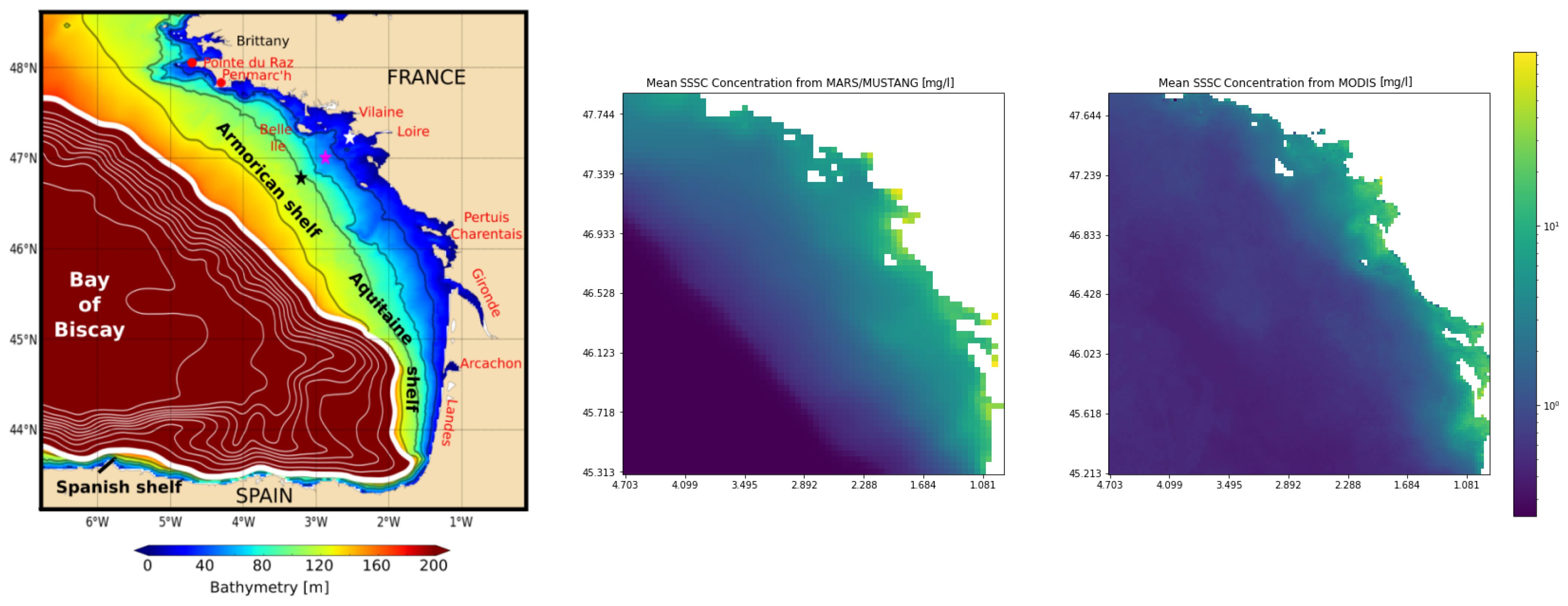
2.1. Area of Interest

The study area encompasses a major part of the northern region of the Bay of Biscay (BoB), located on the west coast of France (North-East Atlantic). In this area the bathymetry extends from the shallow waters of the coast to the great depths of the abyssal plain. The continental shelf is wide (Figure 1). The shelf break, dotted with canyons, crosses the area like a transverse line from its north-west corner to the south-east one. The bottom sedimentology of the BoB can be divided into three main seafloor patterns: a large muddy area located in the middle of the shelf and referred to as the “Grande Vasière” (e.g., [21], coastal areas characterized by rocky and sandy seabeds, and the shelf break with a predominance of rocks. The water column experiences a variety of physical forcings and processes: tides, internal waves (especially from the shelf break), trapped waves, density gradients and seasonal winds driven circulations (with winter storms notably), mixing and stratification, eddies, fronts, filaments, upwelling/downwelling and discharges from rivers [22]. Concerning the latter, the Gironde and Loire rivers are the main sources of water and sediment suspended loads [23]. Their estuaries are located at the northern latitudes of 45.6° and 47.2° respectively. The particle dynamics in the surface layers of this oceanic area is driven by the hydrodynamics superimposed with biologic cycles, which notably are well characterised by phytoplankton blooms appearing along the Armorican shelf break, especially in spring.

2.2. MARS Model Simulations (for OSSE)

The simulations dataset comes from a hydro-sedimentary model called MARS-MUSTANG [21]. MARS is the hydrodynamic module. MUSTANG is the sedimentary module. MARS computes the general circulation according to meteo forcings from meteo models ARPEGE and WaveWatchIII (atmospheric pressure, wind and waves), and density gradients bring by boundary conditions upon climatological dataset. MUSTANG computes sediment resuspension and settling through erosion and deposition laws followed with advection-dispersion and settling velocity equations, in connection with a dynamic seabed sediment layer model, initiated with a nature of seabed chart based on in situ measurements [21]. The main output of this couple model is values of suspended sediment concentrations in the whole water column, from its surface to depths. Since MARS-MUSTANG is designed to model the fate of terrigenous sediments only, the suspended sediment obtained is of mineral (or inorganic) origin, and should appropriately be termed Suspended Particulate Inorganic Matter (SPIM). In particular, SPIM does not include detrital particles because MARS-MUSTANG is not a biological model of primary production with a detrital compartment. Such information on the nature of particles modelled here is necessary when MARS-MUSTANG results are compared with satellite images that “mixes up” more components: especially SPIM and detritus (see following Section 2.3).
Only surface values of suspended sediment concentrations obtained with MARS-MUSTANG will be exploited. In Section 4 (Results), these concentrations will be called using the general term SSSC (surface suspended sediment concentration). For information, these SSSC values were already exploited by our team in order to obtain the present OSSE results in a previous article [19]. This latter article also provides condensed information on the validation of the MARS-MUSTANG simulations with the satellite data, which shows consistent behavior. In particular, the corresponding configuration of the model takes into account the discharges from the two main rivers (Gironde and Loire) and also the Vilaine river (the estuary of which is located slightly north of the Loire one). Figure 1 Middle displays the mean SSSC obtained with the model at the ocean surface and well shows that higher SSSC occurs preferably in the vicinity of the coast. This is due to wave exposure and tidal range in combination with the higher terrigenous sediment loads. Above the abyssal plain, suspended sediments are nearly absent. The threshold of 0.1 mg/L is well correlated with the isobath of 180 m corresponding to the shelf edge. The Figure exhibits area where SSSC values are greater than 10 mg/L near estuaries of the main rivers (Gironde, Loire, Vilaine).
The model is configured with a spatial mesh grid resolution of 2.5 km over a wider area than our area of interest, extending from latitude 41°N to 55°N, and longitude 18°W to 9°30′E [21]. Outputs from MARS-MUSTANG were then extracted in our area of interest, for our present OSSE experiments, and lead to images having a size corresponding to a spatial grid of 128 × 128. In terms of time data frame, the overall sea surface field values extracted from the MARS simulations represent a time series of 1430 daily images spanning from 1 January 2007 to 8 December 2010. The MARS-MUSTANG model and simulations will simply be referred to as MARS hereafter for short.

2.3. MODIS Real Satellite Data (for OSE)

Our satellite-derived dataset is based on the MODIS sensor images acquired on board both Aqua and Terra satellites. The MODIS sensor is part of the 1991 NASA-initiated Earth observation system. It aims at monitoring, among others, the ocean dynamics. Here we exploit the Level-2 geophysical variable called Non-Algal Particles (NAP) that is processed using Francis Gohin et al. bio-optical algorithm [24] applied to the MODIS normalized remote-sensing reflectances. All clouds and cloud shadows in raw satellite images were flagged with a low detection threshold so as to remove all questionable signals. Also, atmospheric over-corrections are taken into account using the reflectance at 412 nm [24]. Their algorithm was specifically calibrated for the Bay of Biscay using dedicated in situ measurements from 20 field cruises that took place over the shelf, and which represent a total amount of about 1000 in situ data points (see Table 1 and Figure 2 of [24]). The NAP concentration (in mg/L) is computed as the difference between the total suspended matter concentration (deduced from the remote-sensing radiances at 550 and 670 nm) and the phytoplankton biomass (derived from their Chlorophyll-a specific algorithm). All products (NAP and Chlorophyll-a) were validated according to additional in situ measurements [25,26]. In particular products accuracy have been extensively validated against coastal in situ measurements from 15 stations located along the French Atlantic coast and 3 stations along the Mediterranean coast, all stations recording the turbidity every 15 days between 1 January 2003 and 31 December 2009. The results show a confidence of 95% (see Figure 13 of [27] in French language) between yearly mean and percentile 90 of the turbidity (in NTU) recorded at all stations and the total suspended matter measured by the MODIS sensor (converted in NTU according to [28]). Part of those results can also be found in English language in [29], including VIIRS (Visible Infrared Imaging Radiometer Suite) and OLCI (Ocean Land color Instrument) satellite sensors, along with MODIS.
For a fine comparison between satellite images and outputs from the MARS model, one should know that the NAP particles observed by the satellite comprise not only mineral particles (labeled as SPIM, see the previous Section 2.2) but also detrital particles, yielding to (e.g., [30]):
NAP = SPIM + d e t ,
where d e t represents the amount of detrital particles. For instance, Figure 1 Right displays the mean SSSC obtained with the satellite (based on the NAP algorithm) at the ocean surface. In particular, it shows that, contrary to the MARS model, there is a weak but significant SSSC mean signal (of the order of 1 mg/L) above the abyssal plain. This signal obviously corresponds to the detrital particles linked to the open sea primary production. Nonetheless, for simplification purposes, in Section 4 (Results) the suspended matter will be called using the general term SSSC (Surface Suspended Sediment Concentration).
In the OSE experiments, our dataset is comprised of daily MODIS images spanning from 1 January 2003 to 31 December 2009. During that period, the mean cloud cover amounted to about 75% of the whole oceanic surface of the imaged area. Each MODIS image has a 1 km spatial resolution, which leads to a 256 × 256 grid for our case-study region. The area extends from latitude 45°17′N to 47°50′N, and longitude 4°55′W to 1°5′W. In terms of validation, as mentioned in Section 2.1, this area covers the main part of the Bay of Biscay (BoB) which experiences various physical and biological forcings. This bay is a well-known fine testing ground in terms of spatial and temporal variability of the turbidity (e.g., [31]).

3. Methods

This section details the proposed space–time interpolation of satellite-derived SSSC fields based on 4DVarNet scheme [32] in Section 3.1, along with the considered evaluation framework, in Section 3.2, performance metrics in Section 3.3 and benchmarked approaches in Section 3.4.

3.1. 4DVarNet Scheme

Deep learning schemes have rapidly become the state-of-the-art approaches for a wide range of pattern recognition and image processing applications, including in geoscience [33]. This also includes neural network approaches dedicated to interpolation issues. Recent studies [17,19,32,34] have stressed the relevance of end-to-end deep learning architectures to address space–time interpolation issues with large missing data rates. Especially, 4DVarNet schemes, which rely on variational data assimilation formulation, have been shown to significantly outperform zero-filling learning-based strategies for interpolation problems [35]. Applications to sea surface height mapping from satellite altimetry [32,34] further support their relevance over other data-driven approaches to better retrieve fine-scale patterns. This study presents an application of 4DVarNet schemes to SSC interpolation. We provide below a short introduction to 4DVarNet schemes. We refer the reader to [18,35] for a detailed presentation.
4DVarNet framework relies on the formulation of the interpolation problem as a variational minimization issue:
x ^ = arg min x y x Ω 2 + λ x Φ ( x ) 2 .
Ω refers to the space–time subdomain where observation y are sampled. Let us point out that we consider a matrix formulation where x and y refer to the space–time process, represented by 2D + t tensors. Operator Φ states the space–time prior to state x. Φ may refer to the flow operator when considering a dynamical ODE or PDE prior. Φ can also derive from a covariance-based prior as in the optimal interpolation framework. Here, following [32], we consider a state-of-the-art neural architecture, namely a UNet [36], such that Φ can be regarded as a projection operator. λ states the relative importance of the observation term of the prior in the minimization problem.
Given minimization problem (2), the 4DVarNet framework implements a trainable iterative gradient-based solver with a predefined number of iterations. As sketched by Figure 2, it delivers an end-to-end architecture which exploits as inputs gappy observation data and as outputs a gap-free state. The trainable solver combines the evaluation of the gradient of variational cost (2) using automatic differentiation tools embedded in deep learning framework with a recurrent network, namely a convolutional LSTM. A more detailed description of 4DVarNet schemes including experiments with different parameterizations of operator Φ and of the trainable solver can be found in [32].
Regarding learning issues, we consider here training losses evaluated on gappy data, as no gap-free reference data are available. For the trainable solver, we consider a convolution LSTM-based solver with a 35-dimensional hidden state.

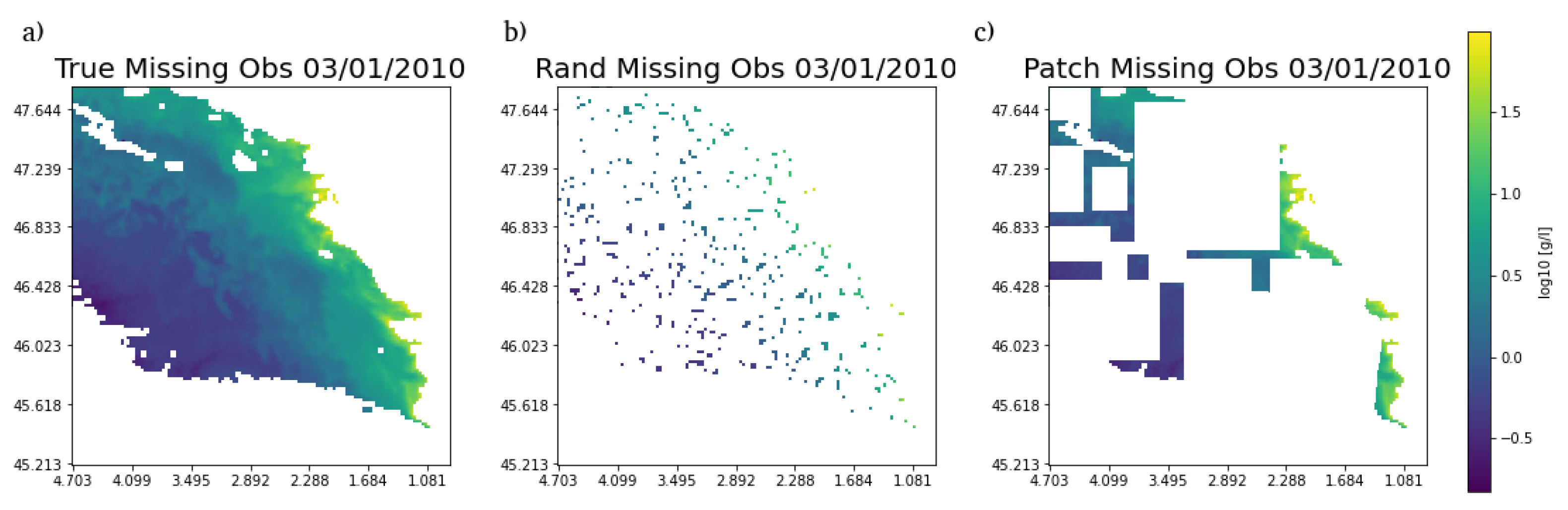
3.2. Training and Evaluation Framework

For training and evaluation purposes, the whole set of data is divided in two parts. All the available data except those of the year 2011 are dedicated to the training while the year 2011 is reserved for the evaluation.
In OSSEs, the “nature run” (or model simulation) provides the reference gap-free field used as ground truth to asses the performance of the interpolation. This helps in evaluating the performance of the associated interpolation methods. For OSEs with real satellite data, no such gap-free reference field is available. We exploit a random sampling strategy as follows. For the considered dataset, we randomly sample a binary mask applied to the real satellite observation patterns. As such, we withhold some observed data from the input data provided to the interpolation methods and use them as reference data to assess reconstruction performance metrics. We may emphasize that this dataset is not an actual groundtruthed dataset as real satellite data are noisy. Available in situ datasets are too scarce to provide a relevant alternative. In the reported experiments, we subsample 50% of available satellite-derived observations for dates at which at least 500 observation points are available (i.e., 3% of the total pixels located above the ocean). We exploit two random strategies: the “pixel-wise” strategy randomly samples 50% of the observed pixels; the “patch-wise” strategy randomly samples H × W patches, width W and height H being randomly sampled according to a uniform distribution between 0 and 100. We report in (Figure 3) examples of randomly sampled patterns. Contrary to the “pixel-wise” strategy, the patch-wise one better matches the expected independence between the training and test datasets.

3.3. Performance Metrics

In terms of performance metrics, we exploit the explained variance (R-score) and the global root mean square error (RMSE) applied to the l o g 10 of concentration values. The latter leads in fact to the RMSLE (root mean square log error) of concentrations, which can be expressed as follows:
R M S L E = 1 n i = 1 n l o g 10 ( C i P r e d ) l o g 10 ( C i O b s ) 2 ,
where C i P r e d are predicted values of SSSC concentrations and C i O b s are the observed values, i stands for the index of evaluated data, n refers to the amount of available observations points. RMSLE and R-Score in all the following Tables are evaluated with a total amount of points of the order of 10 6 . We also evaluate these metrics for the gradient of the l o g 10 of SSSC fields. This validation of results with the standard RMSE on l o g 10 values (i.e., RMSLE) has been chosen for two main reasons:
  • First, the statistical distribution of particle concentrations typically follows a lognormal probability distribution [37] so that l o g 10 values follow a Gaussian distribution. Then, providing bias is negligible (all biases in all experiments were found equal or inferior to 0.01 in absolute values), the RMSE is comparable to a standard deviation and then completely characterizes the statistical distribution;
  • Second, the evaluation on l o g 10 of concentrations emphasizes the validation of low concentrations, which are important in the determination of water transparency, which is a main goal in our studies.

3.4. Reference Methods for Comparison

For benchmarking purposes, we consider two state-of-the-art approaches, an optimal interpolation [38,39] and DINEOF scheme [40]. The Optimal Interpolation (OI), also referred to as kriging, is a method widely applied in ocean remote sensing and geoscience. Numerous operational satellite-derived products in earth science rely on OI. We refer the reader to [41] for a detailed review. In our experiments, we implement an OI with a Gaussian covariance model empirically tuned through cross-validation experiments. DINEOF (Data Interpolating Empirical Orthogonal Functions) is an EOF-based technique for the reconstruction of gap-free fields from irregularly-sampled observations. It has been successfully applied to satellite-derived sea surface products [42], including sea surface turbidity [19,43]. DINEOF iterates a projection–reconstruction step using the EOF basis, while observed variables are kept unchanged after each iteration. Here, we select the first 56 EOF modes to account for 9 ~ 7% of the Variance of the considered datasets and apply a 10-iteration DINEOF. We may point out that the proposed 4DVarNet framework can be regarded as a generalization of DINEOF with a state-dependent covariance model and a gradient-based solver instead of the fixed-point solver implemented by DINEOF [32].

4. Results

We report below the synthesis of the considered numerical experiments. First, a global analysis of all benchmarking experiments is reported in Section 4.1. From these results, Section 4.2 focuses on the comparison between OSSE and OSE performance metrics and Section 4.3 on the performance of our specifically proposed 4DVarNet method.

4.1. Global Performance

Table 1 and Table 2 summarize the performance metrics evaluated with all configurations and interpolation methods. The 4DvarNet method clearly outperformed the other methods tested here for all scores and experiments. For instance, in OSE, when real satellite data are used, 4DvarNet improves R-scores by about 30% w.r.t. OI and 23% w.r.t. DINEOF (slightly depending on the chosen subsampling strategy). We effectively note that reported performance metrics are consistent for the two random sampling strategies used to compute these metrics for the real satellite-derived datasets. The slightly better performance observed with the pixel-wise strategy relates to a lower independence between the input data and the evaluation dataset. A greater stability between the metrics computed according to these two strategies then indicates better generalization properties as exhibited for the 4DVarNet scheme. In OSSE, when simulated data are used, the improvement in R-score with 4DVarNet appears much lower (about 6% w.r.t. OI and 5% w.r.t. DINEOF) but its final R-score is much higher (nearly 97% for OSSE instead of nearly 90% for OSEs). Globally speaking, it appears that R-scores related to OSSE are pretty different to those related to OSEs. This simply reflects the different content in terms of data and data errors between simulated and real satellite images (see the discussion about this subject in Section 5.1. Finally, it is interesting to note the really poor performance of the standard OI method when applied to real data. Indeed, we can see that the correlation between interpolated and real satellite values only amounts to about 60%. Concerning the RMSLE values, Table 2 clearly shows consistent RMSLE values with regard to the R-scores. In particular, OI appears to have low accuracy when applied to real data (around 0.32) and 4DVarNet proved to have the highest accuracy with either simulated or real data (around 0.16 with real data and 0.10 with simulated ones).

4.2. OSSE versus OSE Comparison

Table 3 allows a further analysis on how performance metrics for simulation datasets (OSSE) inform the interpolation performance for real satellite-derived datasets (OSE). The minus signs in front of all values show that, when applied to real satellite data, the accuracy of all tested interpolation methods worsens. Of all interpolation methods, OI loses accuracy the most. This could be due to a misrepresentation of the satellite data noise using this method (see Section 5.1). Concerning the other methods, we point out that OSEs involve an additional complexity at two levels for the training procedure: the reference data are noisy, the reference dataset is gappy. This explains why we also report a lower performance for these methods for OSE settings compared with the OSSE baseline. However, both DINEOF and 4DVarNet lose less accuracy (around 50%) than OI (between 73% and 97%). Thus, OSSE performance metrics provide a sensible assessment of the performance for the real satellite-derived dataset. This is less true for OI, the performance of which is degraded by either 73% or 97% depending on the applied subsampling strategy (Random or Patch). The latter likely relates to the spatial correlation length of the considered covariance model, such that the interpolation capability degrades at a distance greater than the correlation length.

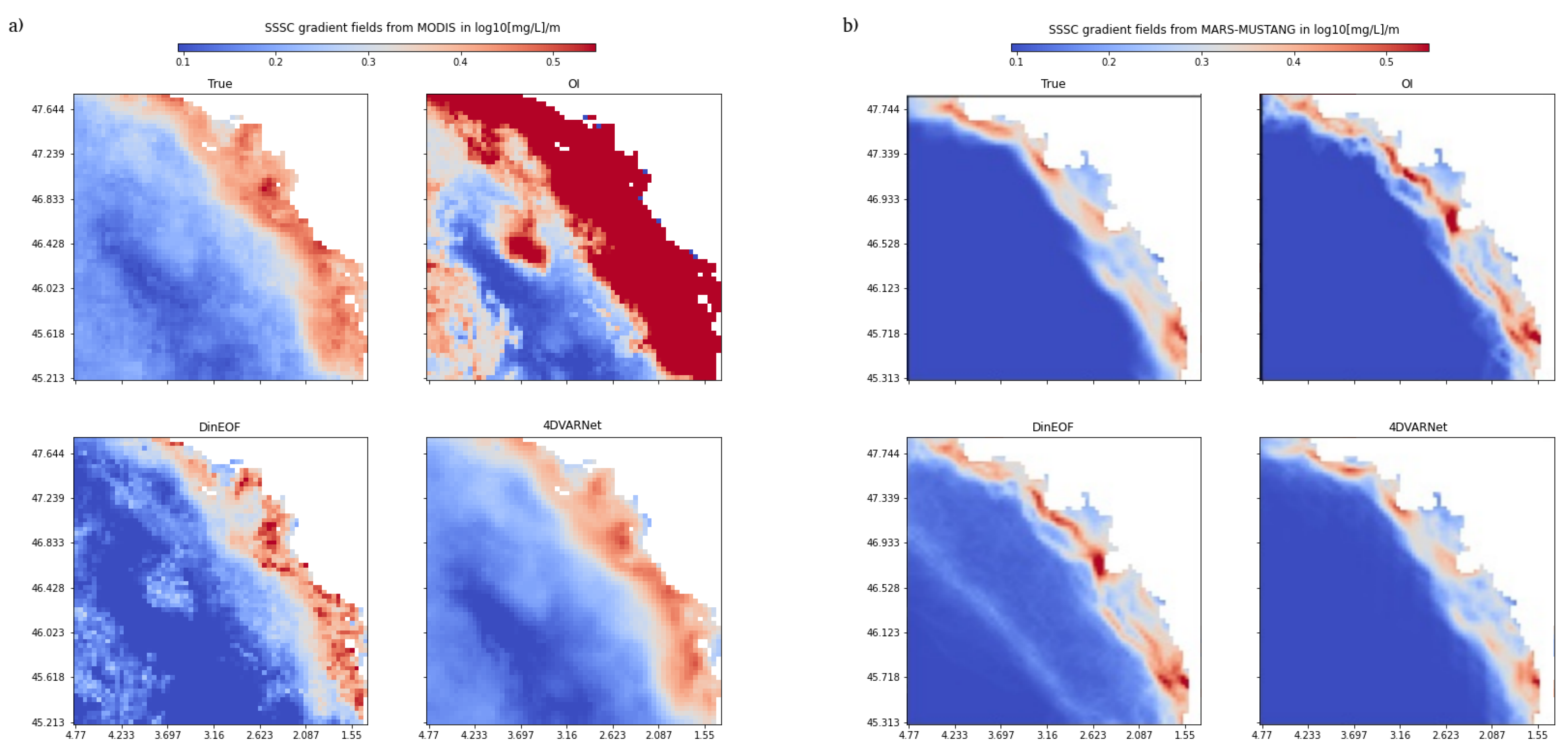
4.3. 4DVarNet Performance

We further analyze the clear improvement reported for 4DVarNet. Table 4 reports the relative performance gains with regard to OI and DINEOF. When dealing with real data, it shows a great improvement of around 50% over OI and a little less, 34%, over DINEOF. These two values quantifying the improvement also appear to be almost insensitive to the subsampling strategy used (Random or Patch). The OSSE is able to quantify a similar amount of improvement over the two methods (OI and DINEOF) with a value of around 40%, but does not see much difference between OI and DINEOF (41% and 38% respectively). This discrepancy between OSSE and OSEs could be due to a different representation of the satellite data noise using OI and DINEOF methods (see Section 5.1).
The evaluation of the interpolation metrics for the gradient of the SSSC fields in Table 5 supports the hypothesis that the improvement obtained with 4DVarNet relates to a better reconstruction of fine-scale patterns. Previous work with similar 4DVar based architecture shows a significant improvement of a high resolution spatial pattern [44]. Surprisingly, the metrics are much better for the OSE. We interpret this aspect as a consequence of the lower spatial variability observed in numerical simulations compared with satellite-derived data, as supported by Figure 4. The mean gradient norm of 4DVarNet nicely recovers the main front structures of the true field compared with the other approaches. More specifically, these gradient fields depict a clearly visible contour offshore. This contour broadly follows the 50 m isobath, which borders the “Grande Vasière”. The OI clearly overestimates the spatial gradient and does not succeed in capturing the finer scale. Though not as bad, DINEOF (based on EOF decomposition) may be limited by the explained variance rate at 97% of the selected EOF components. Besides, for real satellite-derived data, the mean gradient field involves local artifacts. By contrast, 4DVarNet retrieves mean gradient fields which are close to the reference in coastal areas without an overestimation pattern. We can also note a spatial smoothing, which may partially relate to the observation noise of real satellite-derived measurements.

5. Discussion

This study presents and evaluates a novel learning-based interpolation approach referred to as 4DVarNet for the space–time interpolation of satellite-derived sea surface suspended sediment concentrations. Numerical experiments on real and synthetic dataset support the relevance of this scheme compared with state-of-the-art approaches. We further discuss below our main contribution, namely the extent to which OSSEs can inform performance metrics for real datasets (Section 5.1), the relevance of neural network schemes for operational applications (Section 5.2) and the ability to retrieve fine-scale patterns (Section 5.3).

5.1. From OSSE to OSE

A first aim of this study was to compare the performance of interpolation methods when applied to simulated data (through OSSE) and real satellite data (through OSE). At first, the comparison shows that all the methods lost accuracy by a significant amount (more than 40%) when applied to real data. The observation noise in real satellite data may be the driving factor for this pattern. Indeed, in our OSSE, simulated data involve a simple (white) Gaussian noise evenly distributed throughout the whole dataset. By contrast, errors in real satellite data are expected to be much more complex. OI and DINEOF methods may be more impacted as they explicitly or implicitly hypothesize Gaussian noise models. In this retrospect, numerous studies have stressed the ability of neural network approaches to address denoising problems with non-Gaussian noise patterns [33,45].
Beyond the observation noise, other effects may support the difference in performance between OSSE and OSE. For instance, due to the random subsampling strategy, OSSEs involve a slightly lower missing data rate and the reference training data is noise-free. We may also note that we consider a 16-year training time series for OSEs compared with a 4-year one for OSSEs such that the pixel-wise number of training data is the same between OSSEs and OSEs. We may, however, expect a greater intrinsic variability over 16 years which may in turn result in a more complex interpolation problem. We could account for these different aspects in the design of OSSE under the hypothesis that we are provided with longer numerical simulations.
Nevertheless, the numerical simulations used in the OSSEs cannot reveal all the complexity of real satellite data. The hydrosedimentary model does not take into account all the processes we observe in a satellite image. This is of course a major and typically well known drawback of OSSE (e.g., [46]). Here, for instance, a typical discrepancy we can see between the model and a satellite image relates to the biogenic detritus, which follows the dynamics of the oceanic primary production, and which is obviously not modelled by the MARS model (see Equation (1) and the discussion about the difference between SPIM and NAP in Section 2.2 and Section 2.3). Detrital particles can be well observed by satellite remote sensing of ocean color, especially beyond the shelf break (i.e., above the abyssal plain) where the MARS model always shows concentrations (off the shelf) close to zero. Coccolith-derived turbidity is especially amongst the most intense signals detected by a satellite in these areas [47]. Hence, in an OSE, interpolation methods have to address not only the dynamics of purely mineral SPIM particles but also dynamical patterns of detrital particles driven by the primary production.
Finally, we must not forget that the resulting errors in the OSE are biased in the sense that the results are compared with already noisy satellite data, contrary to the OSSE where results are compared with a “true ocean” (the modelled ocean) assumed to be a strict exact solution. Therefore, OSE validation errors are significantly larger than those of the OSSE. However, given these different aspects, the worsening of the interpolation performance of 4DVarNet from the OSSE to the OSE remains fairly limited. This supports the relevance of OSSEs as an initial testbed for the development and evaluation of interpolation algorithms, especially to rank new schemes with respect to previously benchmarked ones within a fully-controlled environment.

5.2. Comparison of Interpolation Methods

Our numerical experiments clearly stress that state-of-the-art data-driven interpolation methods can significantly improve the retrieval of operational gap-free satellite-derived products, which are often based on OI schemes. Both 4DVarNet and DINEOF can account for more complex covariance than the one used by the OI, including anisotropic ones (see in particular [48], for they developed an anisotropic OI method for that case). We believe, however, that a key issue of OI for our case study is its poorer ability to deal with the noise patterns of real satellite-derived observations.
DINEOF performs much better than OI, particularly with real satellite data. This is what our present article demonstrates with the results obtained with the OSE experiments (using real data) compared with what was expected (similar performance between OI and DINEOF) after the OSSE experiments (using simulated data). Furthermore, it has been well demonstrated [17] that DINEOF is well suited for complex areas comprising at the same time coastal and open sea domains. Given that DINEOF is quite simple to implement and does not require strong expertise, this method should definitely be considered as a baseline scheme for routine operational ocean color products similar to those studied in this article. For instance, at a higher spatial resolution, it has recently been applied by the HIGHROC consortium to deliver Sentinel 2 ocean color L4 products corresponding to the CMEMS product OCEANcolor_IBI_BGC_HR_L4_NRT_009_210 (https://doi.org/10.48670/moi-00108, accessed on 12 July 2022) for the IBI area.
4DVarNet further stresses the greater potential of physics-informed learning schemes, which combine some physics-aware representation (here, a variational data assimilation formulation) with the computational efficiency of deep learning. Our results are in line with recent studies dedicated to other satellite-derived products, such as ocean color [49] and satellite altimetry [35]. Compared with [49], 4DVarNet involves an additional modeling flexibility through the learning of a trainable gradient-solver for the variational cost. This also opens the floor to interpolation schemes using multi-source input data through additional trainable observation operators [18]. As such, this work will likely serve as a baseline for future work aiming at further improving the space–time reconstruction of SSSC dynamics.

5.3. Retrieval of Fine-Scale Turbidity Patterns from Satellite Data

Given the irregular sampling of satellite-derived observations, the retrieval of fine-scale patterns is a critical issue for fulfilling operational needs such as the identification of specific areas where waters are highly transparent, which threatens Navy submarines over possible airborne visual detection. Our experiments stress significant differences in the ability of data-driven approaches to retrieve fine-scale patterns. By construction, OI schemes with Gaussian covariance models cannot reconstruct scales smaller than the a priori correlation distance. DINEOF schemes also relate to covariance-based models, but result in more complex covariance models learnt from data. This may actually improve the reconstruction of space–time dynamics. 4DVarNet schemes may be regarded as moving a step further with non-linear quadratic priors through operator Φ in (2), rather than linear-quadratic ones. We regard the combination of such a prior and of a trainable solver as the key features which support the improvement reported for the proposed 4DVarNet schemes.
In our experiments, we exploit RMSE metrics computed for the norm of the gradient of SSSC fields to assess the retrieval of the fine-scale patters. We may note that OSSE scores in Table 5 are significantly lower than the OSE ones, which may be surprising. Numerical simulations involve lower gradient values, whereas real satellite data depict much sharper spatial gradients as illustrated in Figure 4. Given the spatial grid resolution of the MARS model (2.5 km), we expect numerical simulations to resolve spatial scales from 20 km. By contrast, the spatial resolution of MODIS satellite observations is close to 1 km. Besides, as mentioned in Section 5.1, numerical simulations do not include all the processes in play in real satellite observations such as the turbulent behavior in detrital NAP processes. Overall, this results in lower mean gradient norm values for the OSSE, which in turn leads to a lower R-score as this score is normalized by the mean gradient norm. Despite these differences, OSSE and OSE metrics share the same ranking of the benchmarked methods for gradient-related scores. Future developments of hydrosedimentary simulations may improve the ability to reproduce the actual variability of SSSC fields.
Contrary to OI and DINEOF approaches, the proposed 4DVarNet scheme leads to better gradient-based metrics when considering the patch-based random sampling strategy. A similar behavior is observed when applying this method (4DVarNet) to sea surface satellite heights and sea surface temperatures from satellites [44]. In our case, this likely relates to a larger number of training examples with truly observed pixel-level gradients as, by construction, the pixel-level random sampling increases the likelihood that two neighboring pixels are not observed. This further highlights the ability of 4DVarNet schemes to exploit fine-scale patterns in real observation datasets. It also suggests further exploring these random sampling strategies in future work to make the most of available gappy observation datasets.

6. Conclusions

This study presented a novel end-to-end neural scheme for the space–time interpolation of remote sensed sea surface suspended sediment fields, referred to as 4DVarNet. We assessed its reconstruction performance for both real and simulation-based datasets. We reported a clear improvement with respect to the state-of-the-art schemes, namely OI and DINEOF, in terms of global interpolation error of the retrieval of SSSC gradients. To our knowledge, this study is among the few which demonstrate the readiness of end-to-end neural schemes for the processing of L4 gap-free satellite products.
Besides its integration in operational processing pipelines for satellite-derived products, future work could further exploit the variational formulation that 4DVarNet relies on. Through new forcing terms in this variational formulation, it provides a well-posed basis towards the exploitation of forcing variables, for instance associated with wave and barotropic current processes, to further improve the reconstruction of SSSC fields. Similarly, the proposed scheme naturally extends to short-term forecasting applications, which are also of key interest. Overall, we expect this study to serve as a basis for the development of physics-informed deep learning frameworks for ocean remote sensing.

Author Contributions

Conceptualization: R.F., C.D. and F.J.; methodology: R.F.; software: J.-M.V.; validation: J.-M.V. and C.D.; formal analysis: C.D.; writing original draft preparation: J.-M.V.; writing review and editing: F.J., J.-M.V., R.F. and C.D. All authors have read and agreed to the published version of the manuscript.

Funding

This research was funded by the AID (French Agency of Defense Innovation through a PhD scholarship and the city of Brest (BMO). It was supported by ANR Project OceaniX; it was also supported by CNES (French Space Agency) under Project ML4SECCHI (Machine Learning for Secchi visibility). It benefited from HPC and GPU resources from Azure (Microsoft EU Ocean awards).

Data Availability Statement

The computer code and dataset for this study can be found in the https://github.com/Jvient/4DVarNet-OSSE, accessed on 12 July 2022.

Conflicts of Interest

The authors declare that the research was conducted in the absence of any commercial or financial relationships that could be construed as a potential conflict of interest.

Abbreviations

The following abbreviations are used in this manuscript:
ARPEGEAction de Recherche Petite Echelle Grande Echelle
BoBBay of Biscay
CMEMSCopernicus Marine Environment Monitoring Service
DINEOFData INterpolating Empirical Orthogonal function
EOFEmpirical Orthogonal function
HIGHROCHIGH spatial and temporal Resolution Ocean color products and services
IBIIberian-Biscay-Ireland
LSTMLong Short Term Memory
MARSModel for Applications at Regional Scales
MODISModerate-Resolution Imaging Spectroradiometer
MUSTANGMUd and Sand TrAnsport modelliNG
NAPNon-Algal Particles
NNNeural Network
NTUNephelometric Turbidity Unit
OIOptimal Interpolation
OLCIOcean and Land color Instrument
OSEObserving System Experiment (real data)
OSSEObserving System Simulation Experiment (simulated data)
RMSERoot Mean Square Error
RMSLERoot Mean Square Logarithm Error
SPIMSuspended Particulate Inorganic Matter
SSSC(sea) Surface Suspended Sediment Concentration
VIIRSVisible Infrared Imaging Radiometer Suite
4DVarFour-Dimensional Variational data assimilation (model-driven)
4DVarNet    Four-Dimensional Variational (neural) Network data assimilation (data-driven)

References

  1. Owens, P.N. Soil erosion and sediment dynamics in the Anthropocene: A review of human impacts during a period of rapid global environmental change. J. Soils Sediments 2020, 20, 4115–4143. [Google Scholar] [CrossRef]
  2. Irabien, M.J.; Cearreta, A.; Gómez-Arozamena, J.; Gardoki, J.; Martín-Consuegra, A.F. Recent coastal anthropogenic impact recorded in the Basque mud patch (southern Bay of Biscay shelf). Quat. Int. 2020, 566–567, 357–367. [Google Scholar] [CrossRef]
  3. Borja, Á.; Elliott, M.; Carstensen, J.; Heiskanen, A.S.; van de Bund, W. Marine management - Towards an integrated implementation of the European marine strategy framework and the water framework directives. Mar. Pollut. Bull. 2010, 60, 2175–2186. [Google Scholar] [CrossRef]
  4. Elliott, M.; Borja, Á.; McQuatters-Gollop, A.; Mazik, K.; Birchenough, S.; Andersen, J.H.; Painting, S.; Peck, M. Force majeure: Will climate change affect our ability to attain Good Environmental Status for marine biodiversity? Mar. Pollut. Bull. 2015, 95, 7–27. [Google Scholar] [CrossRef] [PubMed]
  5. Larcombe, P.; Morrison-Saunders, A. Managing marine environments and decision-making requires better application of the physical sedimentary sciences. Australas. J. Environ. Manag. 2017, 24, 200–221. [Google Scholar] [CrossRef]
  6. Tecchiato, S.; Collins, L.; Parnum, I.; Stevens, A. The influence of geomorphology and sedimentary processes on benthic habitat distribution and littoral sediment dynamics: Geraldton, Western Australia. Mar. Geol. 2015, 359, 148–162. [Google Scholar] [CrossRef]
  7. James, I.D. Modelling pollution dispersion, the ecosystem and water quality in coastal waters: A review. Environ. Model. Softw. 2002, 17, 363–385. [Google Scholar] [CrossRef]
  8. Mitchell, C.; Cunningham, A. Remote sensing of spatio-temporal relationships between the partitioned absorption coefficients of phytoplankton cells and mineral particles and euphotic zone depths in a partially mixed shelf sea. Remote Sens. Environ. 2015, 160, 193–205. [Google Scholar] [CrossRef]
  9. Saulnier, J.B.; Escobar-Valencia, E.; Grognet, M.; Waeles, B. 3D Modelling for the Dispersion of Sediments Dredged in the Port of La Rochelle with Open TELEMAC-MASCARET. In Proceedings of the Papers Submitted to the 2020 TELEMAC-MASCARET User Conference, Antwerp, Belgium, 14–15 October 2021; pp. 129–137. [Google Scholar]
  10. Diaz, M.; Grasso, F.; Le Hir, P.; Sottolichio, A.; Caillaud, M.; Thouvenin, B. Modeling Mud and Sand Transfers Between a Macrotidal Estuary and the Continental Shelf: Influence of the Sediment Transport Parameterization. J. Geophys. Res. Ocean. 2020, 125, 1–37. [Google Scholar] [CrossRef]
  11. Le Hir, P.; Monbet, Y.; Orvain, F. Sediment erodability in sediment transport modelling: Can we account for biota effects? Cont. Shelf Res. 2007, 27, 1116–1142. [Google Scholar] [CrossRef]
  12. Wang, Y.P.; Voulgaris, G.; Li, Y.; Yang, Y.; Gao, J.; Chen, J.; Gao, S. Sediment resuspension, flocculation, and settling in a macrotidal estuary. J. Geophys. Res. Ocean. 2013, 118, 5591–5608. [Google Scholar] [CrossRef]
  13. Renosh, P.R.; Jourdin, F.; Charantonis, A.A.; Yala, K.; Rivier, A.; Badran, F.; Thiria, S.; Guillou, N.; Leckler, F.; Gohin, F.; et al. Construction of multi-year time-series profiles of suspended particulate inorganic matter concentrations using machine learning approach. Remote Sens. 2017, 9, 1320. [Google Scholar] [CrossRef]
  14. Moore, A.M.; Martin, M.J.; Akella, S.; Arango, H.G.; Balmaseda, M.; Bertino, L.; Ciavatta, S.; Cornuelle, B.; Cummings, J.; Frolov, S.; et al. Synthesis of ocean observations using data assimilation for operational, real-time and reanalysis systems: A more complete picture of the state of the ocean. Front. Mar. Sci. 2019, 6, 90. [Google Scholar] [CrossRef]
  15. Nazeer, M.; Bilal, M.; Alsahli, M.; Shahzad, M.; Waqas, A. Evaluation of Empirical and Machine Learning Algorithms for Estimation of Coastal Water Quality Parameters. ISPRS Int. J. Geo-Inf. 2017, 6, 360. [Google Scholar] [CrossRef]
  16. Jin, D.; Lee, E.; Kwon, K.; Kim, T. A Deep Learning Model Using Satellite Ocean Color and Hydrodynamic Model to Estimate Chlorophyll- a Concentration. Remote Sens. 2021, 13, 2003. [Google Scholar] [CrossRef]
  17. Barth, A.; Alvera-Azcárate, A.; Troupin, C.; Beckers, J.M. DINCAE 2.0: A convolutional neural network with error estimates to reconstruct sea surface temperature satellite observations. Geosci. Model Dev. 2022, 15, 2183–2196. [Google Scholar] [CrossRef]
  18. Fablet, R.; Beauchamp, M.; Drumetz, L.; Rousseau, F. Joint Interpolation and Representation Learning for Irregularly Sampled. Front. Appl. Math. Stat. 2021, 7, 655224. [Google Scholar] [CrossRef]
  19. Vient, J.M.; Jourdin, F.; Fablet, R.; Mengual, B.; Lafosse, L.; Delacourt, C. Data-driven interpolation of sea surface suspended concentrations derived from ocean color remote sensing data. Remote Sens. 2021, 13, 3537. [Google Scholar] [CrossRef]
  20. Mengual, B.; Hir, P.L.; Cayocca, F.; Garlan, T. Modelling fine sediment dynamics: Towards a common erosion law for fine sand, mud and mixtures. Water 2017, 9, 564. [Google Scholar] [CrossRef]
  21. Mengual, B.; Le Hir, P.; Cayocca, F.; Garlan, T. Bottom trawling contribution to the spatio-temporal variability of sediment fluxes on the continental shelf of the Bay of Biscay (France). Mar. Geol. 2019, 414, 77–91. [Google Scholar] [CrossRef]
  22. Huthnance, J.; Hopkins, J.; Berx, B.; Dale, A.; Holt, J.; Hosegood, P.; Inall, M.; Jones, S.; Loveday, B.R.; Miller, P.I.; et al. Ocean shelf exchange, NW European shelf seas: Measurements, estimates and comparisons. Prog. Oceanogr. 2022, 202, 102760. [Google Scholar] [CrossRef]
  23. Castaing, P.; Froidefond, J.M.; Lazure, P.; Weber, O.; Prud’Homme, R.; Jouanneau, J.M. Relationship between hydrology and seasonal distribution of suspended sediments on the continental shelf of the Bay of Biscay. Deep-Sea Res. Part II Top. Stud. Oceanogr. 1999, 46, 1979–2001. [Google Scholar] [CrossRef]
  24. Gohin, F.; Loyer, S.; Lunven, M.; Labry, C.; Froidefond, J.M.; Delmas, D.; Huret, M.; Herbland, A. Satellite-derived parameters for biological modelling in coastal waters: Illustration over the eastern continental shelf of the Bay of Biscay. Remote Sens. Environ. 2005, 95, 29–46. [Google Scholar] [CrossRef]
  25. Gohin, F.; Saulquin, B.; Oger-Jeanneret, H.; Lozac’h, L.; Lampert, L.; Lefebvre, A.; Riou, P.; Bruchon, F. Towards a better assessment of the ecological status of coastal waters using satellite-derived chlorophyll-a concentrations. Remote Sens. Environ. 2008, 112, 3329–3340. [Google Scholar] [CrossRef]
  26. Petus, C.; Chust, G.; Gohin, F.; Doxaran, D.; Froidefond, J.M.; Sagarminaga, Y. Estimating turbidity and total suspended matter in the Adour River plume (South Bay of Biscay) using MODIS 250-m imagery. Cont. Shelf Res. 2010, 30, 379–392. [Google Scholar] [CrossRef]
  27. Gohin, F.; Saulquin, B.; Bryere, P. Atlas de la Température, de la Concentration en Chlorophylle et de la Turbidité de Surface du Plateau Continental Français et de ses Abords de L’Ouest Européen. 2010, p. 53. Available online: https://archimer.ifremer.fr/doc/00057/16840/14306.pdf (accessed on 12 July 2022).
  28. Nechad, B.; Ruddick, K.G.; Park, Y. Calibration and validation of a generic multisensor algorithm for mapping of total suspended matter in turbid waters. Remote Sens. Environ. 2010, 114, 854–866. [Google Scholar] [CrossRef]
  29. Gohin, F.; Bryère, P.; Lefebvre, A.; Sauriau, P.G.; Savoye, N.; Vantrepotte, V.; Bozec, Y.; Cariou, T.; Conan, P.; Coudray, S.; et al. Satellite and in situ monitoring of chl-a, turbidity, and total suspended matter in coastal waters: Experience of the year 2017 along the french coasts. J. Mar. Sci. Eng. 2020, 8, 665. [Google Scholar] [CrossRef]
  30. Bellacicco, M.; Cornec, M.; Organelli, E.; Brewin, R.J.; Neukermans, G.; Volpe, G.; Barbieux, M.; Poteau, A.; Schmechtig, C.; D’Ortenzio, F.; et al. Global Variability of Optical Backscattering by Non-algal particles From a Biogeochemical-Argo Data Set. Geophys. Res. Lett. 2019, 46, 9767–9776. [Google Scholar] [CrossRef]
  31. Borja, A.; Amouroux, D.; Anschutz, P.; Gómez-Gesteira, M.; Uyarra, M.C.; Valdés, L. The Bay of Biscay, 2nd ed.; Elsevier Ltd.: Amsterdam, The Netherlands, 2018; pp. 113–152. [Google Scholar] [CrossRef]
  32. Fablet, R.; Drumetz, L.; Rousseau, F.; Fablet, R.; Drumetz, L.; End-to end, F.R. End-to-End Learning of Variational Models and Solvers for the Resolution of Interpolation Problems. 2021. Available online: https://hal-imt-atlantique.archives-ouvertes.fr/hal-03139133/document (accessed on 12 July 2022).
  33. Zhang, L.; Zhang, L.; Du, B. Deep learning for remote sensing data: A technical tutorial on the state of the art. IEEE Geosci. Remote Sens. Mag. 2016, 4, 22–40. [Google Scholar] [CrossRef]
  34. Beauchamp, M.; Fablet, R.; Ubelmann, C.; Ballarotta, M.; Chapron, B. Intercomparison of data-driven and learning-based interpolations of along-track nadir and wide-swath swot altimetry observations. Remote Sens. 2020, 12, 3806. [Google Scholar] [CrossRef]
  35. Fablet, R.; Chapron, B.; Drumetz, L.; Memin, E.; Pannekoucke, O.; Rousseau, F. Learning Variational Data Assimilation Models and Solvers. arXiv 2020, arXiv:2007.12941. [Google Scholar] [CrossRef]
  36. Gao, Y.; Guan, J.; Zhang, F.; Wang, X.; Long, Z. Attention-Unet-Based Near-Real-Time Precipitation Estimation from Fengyun-4A Satellite Imageries. Remote Sens. 2022, 14, 2925. [Google Scholar] [CrossRef]
  37. Eleveld, M.A.; Pasterkamp, R.; van der Woerd, H.J.; Pietrzak, J.D. Remotely sensed seasonality in the spatial distribution of sea-surface suspended particulate matter in the southern North Sea. Estuar. Coast. Shelf Sci. 2008, 80, 103–113. [Google Scholar] [CrossRef]
  38. Daley, R. Atmospheric data Assimilation. J. Meterolog. Soc. Jpn. 1997, 75, 319–329. [Google Scholar] [CrossRef]
  39. Cressie, N.A.C.; Wikle, C.K. Statistics for Spatio-Temporal Data; Wiley: Hoboken, NJ, USA, 2011; p. 588. [Google Scholar]
  40. Beckers, J.M.; Rixen, M. EOF calculations and data filling from incomplete oceanographic datasets. J. Atmos. Ocean. Technol. 2003, 20, 1839–1856. [Google Scholar] [CrossRef]
  41. OLIVER, M.A.; WEBSTER, R. Kriging: A method of interpolation for geographical information systems. Int. J. Geogr. Inf. Syst. 2007, 4, 313–332. [Google Scholar] [CrossRef]
  42. Alvera-Azcárate, A.; Vanhellemont, Q.; Ruddick, K.; Barth, A.; Beckers, J.M. Analysis of high frequency geostationary ocean color data using DINEOF. Estuar. Coast. Shelf Sci. 2015, 159, 28–36. [Google Scholar] [CrossRef]
  43. Liu, X.; Wang, M. Analysis of ocean diurnal variations from the Korean Geostationary Ocean Color Imager measurements using the DINEOF method. Estuar. Coast. Shelf Sci. 2016, 180, 230–241. [Google Scholar] [CrossRef]
  44. Fablet, R.; Febvre, Q.; Chapron, B. Multimodal 4DVarNets for the reconstruction of sea surface dynamics from SST-SSH synergies. arXiv 2022, arXiv:2207.01372. [Google Scholar]
  45. Guo, X.; Liu, X.; Zhu, E.; Yin, J. Deep Clustering with Convolutional Autoencoders. In Lecture Notes in Computer Science (Including Subseries Lecture Notes in Artificial Intelligence and Lecture Notes in Bioinformatics), Proceedings of the 24th International Conference, ICONIP 2017, Guangzhou, China, 14–18 November 2017; Springer: Berlin/Heidelberg, Germany, 2017. [Google Scholar] [CrossRef]
  46. Hoffman, R.N.; Atlas, R. Future observing system simulation experiments. Bull. Am. Meteorol. Soc. 2016, 97, 1601–1616. [Google Scholar] [CrossRef]
  47. Perrot, L.; Gohin, F.; Ruiz-Pino, D.; Lampert, L.; Huret, M.; Dessier, A.; Malestroit, P.; Dupuy, C.; Bourriau, P. Coccolith-derived turbidity and hydrological conditions in May in the Bay of Biscay. Prog. Oceanogr. 2018, 166, 41–53. [Google Scholar] [CrossRef]
  48. Saulquin, B.; Gohin, F.; Fanton d’Andon, O. Interpolated fields of satellite-derived multi-algorithm chlorophyll-a estimates at global and European scales in the frame of the European Copernicus-Marine Environment Monitoring Service. J. Oper. Oceanogr. 2019, 12, 47–57. [Google Scholar] [CrossRef]
  49. Barth, A.; Alvera-Azcárate, A.; Licer, M.; Beckers, J.M. DINCAE 1.0: A convolutional neural network with error estimates to reconstruct sea surface temperature satellite observations. Geosci. Model Dev. 2020, 13, 1609–1622. [Google Scholar] [CrossRef]
Figure 1. (Left) Bathymetry of the Bay of Biscay. Black lines represent isobaths 40, 70, 100, and 130 m. The thick white line (corresponding to the 180 m isobath) approximately delimits the shelf edge. Stars are validation points in [21] (Middle) Mean spatial distribution of SSSC (in mg/L) from the MARS-MUSTANG hydrosedimentary model. (Right) Mean spatial distribution of SSSC (in mg/L) from MODIS observations.
Remotesensing 14 04024 g001
Figure 2. Workflow of the proposed framework for the reconstruction NAP field with the 4DVarNet. A given observation dataset catalogue is provide for the learning phase of the model. The interpolator Φ is trained and optimised by the solver. Then the model is able to reconstruct the irregularly sampled time series input into the reconstructed data.
Remotesensing 14 04024 g002
Figure 3. Different sampling strategy for validation by using missing observations: (a) True observation from MODIS L2 image dataset (b) Random points sampling strategy for observation sampling (c) Patch sampling strategy for observation sampling.
Remotesensing 14 04024 g003
Figure 4. Reconstruction norm of SSSC gradient fields for the OSE (MODIS) and OSSE (MARS) application for the whole validation period: (a) OSE configuration (b) OSSE configuration.
Remotesensing 14 04024 g004
Table 1. R-score performance in % for the considered methods and validation configurations. OSE refers to the real data (MODIS) interpolating process. The sub-sampling strategy is described in Section 3.2. OSSE dataset refers to the previous work [19] based on the MARS results.
ExperimentDatasetSub-SamplingOIDINEOF4DVarNet
OSEMODISRandom60.576.489.5
OSEMODISPatch56.573.887.3
OSSEMARS-90.491.396.6
Table 2. RMSLE performance in l o g 10 [mg/L] for the considered methods and validation configurations. OSE refers to the real data (MODIS) interpolating process. The sub-sampling strategy is described in Section 3.2. OSSE dataset refers to the previous work [19] based on the MARS results.
ExperimentDatasetSub-SamplingOIDINEOF4DVarNet
OSEMODISRandom0.3040.2370.156
OSEMODISPatch0.3460.2530.168
OSSEMARS-0.1760.1670.104
Table 3. Evolution of accuracy, from OSSE to OSE, in the form of a performance rate according to the formula 1 − RMSLE(OSE)/RMSLE(OSSE) expressed in percentage, using the RMSLE reported in Table 2.
Sub-SamplingOIDINEOF4DVarNet
Random−73%−42%−50%
Patch−97%−51%−62%
Table 4. Evolution of accuracy, from OI or DINEOF to 4DVarNet, in the form of a performance rate according to the formula 1 − RMSLE(4DVarNet)/RMSLE(·) expressed in percentage, when using the RMSLE reported in Table 2.
ExperimentDatasetSub-SamplingOIDINEOF
OSEMODISRandom49%34%
OSEMODISPatch51%34%
OSSEMARS-41%38%
Table 5. Gradient norm reconstruction performance R-score evaluation for different methods and validation configurations in %. OSSE dataset refers to the previous work ([19]) based on the MARS/MUSTANG results in an OSSE application. MODIS dataset refers to the real data interpolating process, with learning based only on observations. The sub-sampling strategy is described in Section 3.2.
ExperimentDatasetSub-SamplingOIDINEOF4DVarNet
OSEMODISRandom58.372.588.9
OSEMODISPatch56.667.491.2
OSSEMARS-16.040.663.7
Publisher’s Note: MDPI stays neutral with regard to jurisdictional claims in published maps and institutional affiliations.

