Prediction of Sea Surface Temperature in the East China Sea Based on LSTM Neural Network

Abstract

Sea surface temperature (SST) is an important physical factor in the interaction between the ocean and the atmosphere. Accurate monitoring and prediction of the temporal and spatial distribution of SST are of great significance in dealing with climate change, disaster prevention, disaster reduction, and marine ecological protection. This study establishes a prediction model of sea surface temperature for the next five days in the East China Sea using long-term and short-term memory neural networks (LSTM). It investigates the influence of different parameters on prediction accuracy. The sensitivity experiment results show that, based on the same training data, the length of the input data of the LSTM model can improve the model’s prediction performance to a certain extent. However, no obvious positive correlation is observed between the increase in the input data length and the improvement of the model’s prediction accuracy. On the contrary, the LSTM model’s performance decreases with the prediction length increase. Furthermore, the single-point prediction results of the LSTM model for the estuary of the Yangtze River, Kuroshio, and the Pacific Ocean are accurate. In particular, the prediction results of the point in the Pacific Ocean are the most accurate at the selected four points, with an RMSE of 0.0698 °C and an $R^2$ of 99.95%. At the same time, the model in the Pacific region is migrated to the East China Sea. The model was found to have good mobility and can well represent the long-term and seasonal trends of SST in the East China Sea.

1. Introduction

Sea surface temperature (SST) plays a vital role in the energy balance of the earth’s surface and the exchange of energy, momentum, and moisture between the ocean and atmosphere [1,2]. It could affect the precipitation distribution, leading to extreme weather events, such as droughts and floods [3,4]. The variation of SST would also affect biological processes, such as the distribution and reproduction of marine organisms; it can also impact marine ecosystems [5,6,7,8,9,10]. The accurate prediction of SST is of great significance in marine disaster prevention and mitigation, ecological protection, and response to global climate change.

The East China Sea (ECS) is a marginal sea of the Northwest Pacific [11]. It is located east of the China mainland, south of the Yellow Sea, and north of the South China Sea, with an area of about 770,000 km². The SST of ECS is affected by the East Asian monsoon system, with an annual average water temperature between 20 °C and 24 °C and an annual temperature difference between 7 °C and 9 °C. In addition to being affected by the monsoon climate, the SST of the ECS is also affected by the tidal system and the complex circulation in the ECS, such as the Kuroshio Current, the Taiwan Warm Current, the Zhejiang-Fujian Coastal Current, and the Tsushima Warm Current [12]. The change of SST is extremely complex. Moreover, the ECS is also one of the most important areas for marine heat wave disasters [13]. The prediction of SST is of great significance to the local hydrology and ecological environment. It also provides an important basis for predicting and warning of marine heat wave disasters in the ECS under climate warming.

Currently, the SST prediction methods are mainly divided into two categories. One is to use ocean numerical models. For example, Gao et al. [13] used the Finite-Volume Coastal Ocean Model (FVCOM) to study marine heatwaves in the East China Sea and the South Yellow Sea. Tiwari et al. [14] used the Regional Ocean Modeling System (ROMS) to study the sea surface temperature of the Indian Ocean. Gao et al. [15] used the HYbrid Coordinate Ocean Model (HYCOM) to simulate the sea surface temperature of the tropical and North Pacific basins. These oceanic numerical models had been established through kinetic and thermal equations and obtained the numerical solution with initial conditions and boundary conditions [16]. In terms of improving the accuracy of numerical models, the higher the accuracy, the more complex the numerical model and the higher the computational cost, which leads to the need for a large number of computing resources and relevant professional personnel to carry out the operational SST prediction work [17]. The second is adopting a data-driven approach, including traditional statistical methods and the latest machine learning methods. Traditional statistical methods, such as the Markov model [18], regression model [19], and empirical canonical correlation analysis, etc., [20], can reflect the changing law of data to a certain extent based on specific observation data and have the characteristics of a small calculation amount, but they are difficult to improve the prediction accuracy [21]. In recent years, machine learning methods have gradually become popular with the increased SST data and the rapid advance in computer technology. The current popular machine learning methods include decision trees [22], random forests [23], artificial neural networks [24], and support vector machines, etc., [25]. The machine learning method is done to discover the law of data changes from a large amount of observation data. Compared with the traditional statistical method, the prediction accuracy is significantly improved. It also has the advantages of low computational cost and easy parameterization to other geographic locations. Furthermore, the demand for this method for marine professional knowledge is not as high as that of marine numerical prediction.

Among the popular machine learning methods, neural network models are widely used because of their flexibility and powerful modeling ability [26,27]. Tang et al. [28,29,30] applied the neural network method to the prediction of SST for the first time. They used a feed-forward neural network to predict the average sea surface temperature anomalies in the Niño region, showing that the neural network is excellent in capturing nonlinear relationships. Then, Wu et al. [31] established a nonlinear sea surface temperature anomalies prediction model using the multilayer back propagation (BP) neural network method combined with empirical mode decomposition (EMD), which proved that its correlation skills are enhanced by 0.10–0.14 compared with the linear regression model. Gupta and Malmgren [32] made a comparative study on the prediction ability of various methods relying on specific training algorithms, regression, and artificial neural networks, and showing that the RMSEP value of the neural network was 1.3 °C, which was better than other algorithms. Tripathi et al. [33] used an artificial neural network to predict sea surface temperature anomalies in a small area of the Indian Ocean and found that the model could predict sea surface temperature anomalies with considerable accuracy. Furthermore, Patil and De [34,35], Mohongo and Deo et al. [36] also used the neural network to predict SST, showing that the neural network has a certain improvement compared with traditional statistical methods. Aparna et al. [37] proposed a neural network consisting of three layers, an input layer, a linear layer, and an output layer to predict the SST of the next day at a specific location, and found that the error of the prediction is within ±0.5 °C. However, most use traditional neural networks, which have a relatively simple structure and limited learning ability. Thus, they cannot describe the complex features in the data well. At the same time, they also have shortcomings, such as low training efficiency and the inability to fully use a large amount of SST data to train prediction models [38], which are being replaced by neural networks with deeper layers.

As a typical representative of the deep neural network in long-term sequence, the long short-term memory neural network (LSTM) model has a lower computational cost and less requirement for marine expertise than the numerical model. Compared with a shallow neural network, the LSTM model has a more complex structure to extract data change rules better. Compared with the Recurrent Neural Network (RNN), which deals with time-series data, it can prevent the gradient disappearance and explosion in the backpropagation process [39]. The reason is that, under the action of the gating mechanism, LSTM can better capture long-time series data. Therefore, it is widely used in time series forecasting problems. Zhang et al. [40] used daily, weekly, and monthly SST data to forecast the Bohai Sea one day, three days, one week, and one month in advance. The results show that the LSTM model captures time-series information better than the traditional multilayer feed-forward network. To the best of our knowledge, they are the first to apply LSTM networks to SST prediction. Sarkar [41] also applied the LSTM model to SST prediction and found that the correlation coefficient (r) between the predicted value and the actual value is close to 1. Kim et al. [42] used the LSTM model to predict the SST in the coastal areas of South Korea and found that the RMSE of the LSTM model one day in advance is about 0.4 °C. Their prediction results are of great significance for the prevention of aquaculture. Li [43] used the LSTM model to predict the SST in the sea area where El Niño or La Niña occurred, and the correlation coefficient between the predicted value and the actual value reached 94%, which provided a noteworthy method for the monitoring and prediction of El Niño or La Niña. Of course, there are also many scholars who use the LSTM model with other methods to predict SST. For example, Xiao et al. [44,45], respectively, applied the LSTM-AdaBoost and ConvLSTM models to SST prediction in ECS and found that the LSTM-AdaBoost and ConvLSTM models have good application prospects for medium- and short-term SST prediction. Wei et al. [46] used a self-organizing mapping (SOM) algorithm to divide the entire China Sea and its adjacent areas into 130 small areas. Then, they built an LSTM model for each area to predict its SST and found that, one month in advance, the root mean square error (RMSE) of the prediction is 0.5 °C. Sun et al. [47] combined the graph convolutional neural network (GCN) with the LSTM neural network to create a time-series graph network (TSGN) to predict SST and found that the RMSE predicted 3 days in advance is 0.47 °C. Zhang et al. [48] used the gated recurrent unit (GRU) model to predict the SST in the Bohai Sea and found that it can effectively fit the actual SST, with a correlation coefficient of 0.98. However, the above studies did not explore the impact of input and prediction lengths on the accuracy of LSTM models and the model’s mobility.

This paper discusses the impact of input lengths and prediction lengths of SST on the prediction performance of the LSTM model and the application of the single-point prediction model of SST in a small area, which provides a reference for the operational prediction of SST, marine pasture, aquaculture, and other industries greatly affected by sea surface temperature, especially for some aquaculture industries with simple equipment in ECS. The specific content of the experiment is as follows: (1) A set of sensitivity experiments on input and prediction lengths are designed, and the influence of input and prediction lengths on the prediction results of the LSTM model is analyzed through the results of sensitivity experiments. (2) Through a training model at a specific location to predict the SST of ECS, experiments show that more than 95% of the RMSE values predicted by this method 5 days in advance are within 0.4 °C. Compared with the experimental results shown by the model proposed by Zhang et al. [40], which combines the SOM algorithm with the LSTM model, the TSGCN model proposed by Sun et al. [41], and Xiao et al. [47] applied ConvLSTM to prediction of SST, the RMSE value of this experiment decreased by 0.1, 0.07, 0.25, respectively.

The remainder of this paper is structured as follows. Section 2 describes the satellite data and the LSTM model used in this study. Section 3 presents the experimental results and a detailed discussion. Section 4 gives the conclusion.

2. Materials and Methods

There are many sources of observation data. Compared with buoy data, high-resolution satellite data is easier to obtain. In this section, we introduce the data sources and LSTM method in detail. The details are as follows:

2.1. Materials

The high-resolution satellite remote sensing sea surface temperature data used in this study is Operational Sea Surface Temperature and Sea Ice Analysis (OSTIA). OSTIA is the operational sea temperature and sea ice analysis system [49]. Based on the data provided by Group for high resolution sea surface temperature (GHRSST), it is a daily 1/20° grid SST product made by the UK Met Office using AATSR data, SEVIRI data, AVHRR data, AMSR data, TMI data, and in situ measurements. All satellite SST data are adjusted for bias errors based on a combination of AATSR SST data and in situ SST measurements from drifting buoys. The product is generated by using an optimal algorithm, and its RMSE is less than 0.6 °C [50]. The spatial range of SST data used in this study is (22°N–33°N, 120°E–131°E), and the time range is 2010–2020, of which the SST data from 2010–2019 is the training data and validation data, and SST data in 2020 is the test data.

2.2. Methods

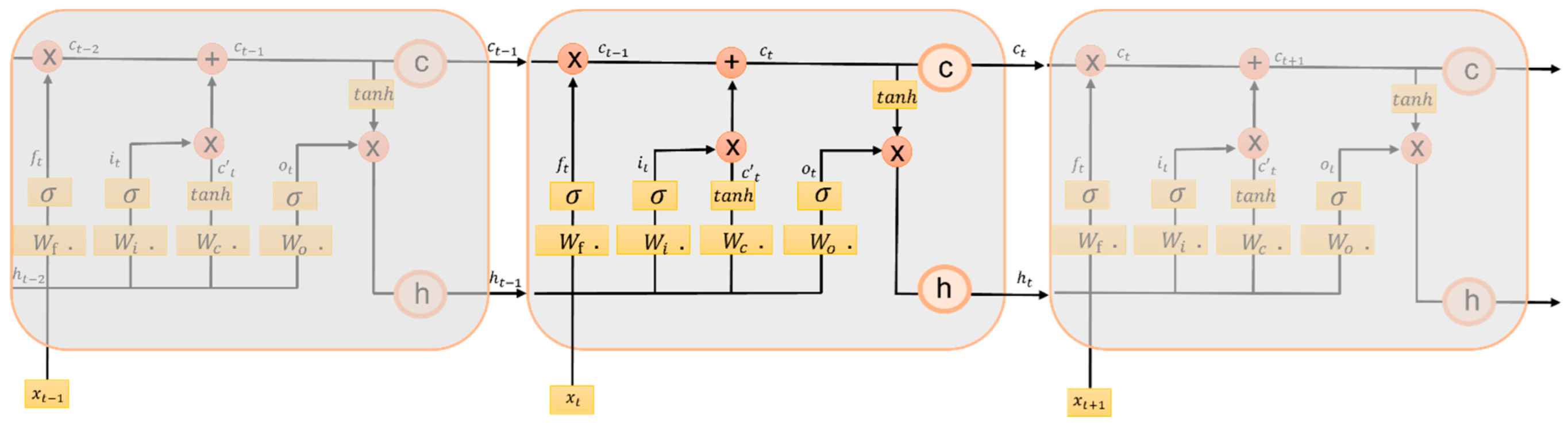
2.2.1. LSTM Neural Network

LSTM is a special form of RNN, proposed by Hochreiter and Schmidhuber in 1997 [51]. LSTM overcomes, to some extent, the most direct gradient disappearance or explosion problem caused by a traditional RNN due to an excessive number of layers in the time dimension. The main reason is that LSTM network introduces a unit state and uses a gating mechanism to save and control information flow. The cell structure is shown in Figure 1. Its first gate is the forget gate, which determines how much of the cell state $C_{t-1}$ at the previous moment is retained to the current moment $C_t$. The second gate is the input gate, which determines how much of the network input $X_t$ at the current moment is saved to the cell state $C_t$. The third gate is the output gate, which controls how much of the unit state$C_t$ is exported to the current output value $h_t$ of the LSTM. The gating mechanism and the update computation of the cell state are as follows:

Forgotten gate:

$$f_t=\sigma (W_f.[h_{t-1},x_t]+b_f)$$

(1)

Input gate:

$$i_t=\sigma (W_i.[h_{t-1},x_t]+b_i)$$

(2)

$${C^{\prime }}_t=tanh\left(W_c.[h_{t-1},x_t\right]+b_c)$$

(3)

$$C_t=f_t\ast C_{t-1}+i_t\ast {C^{\prime }}_t$$

(4)

Output gate:

$$o_t=\sigma (W_o.[h_{t-1},x_t]+b_o)$$

(5)

$$h_t=o_t\ast tanh\left(C_t\right)$$

(6)

where $h_{t-1}$ represents the output value of the hidden layer at the previous moment, and $x_t$ is the current input value. $\sigma$ and tanh are activation functions, and σ represents the sigmoid function. $f_t$, $i_t$, and $o_t$ denote forgetting gate values, enter threshold values, and output gate values. $W_f$, $W_i$, $W_c$, and $W_o$ are weight matrices. $b_f$, $b_i$, $b_c$, and $b_o$ are the corresponding offset terms. $C_{t-1}$, ${C^{\prime }}_t$, and $C_t$ represents the cell state at the previous time, the candidate state, and the cell state at the current time.

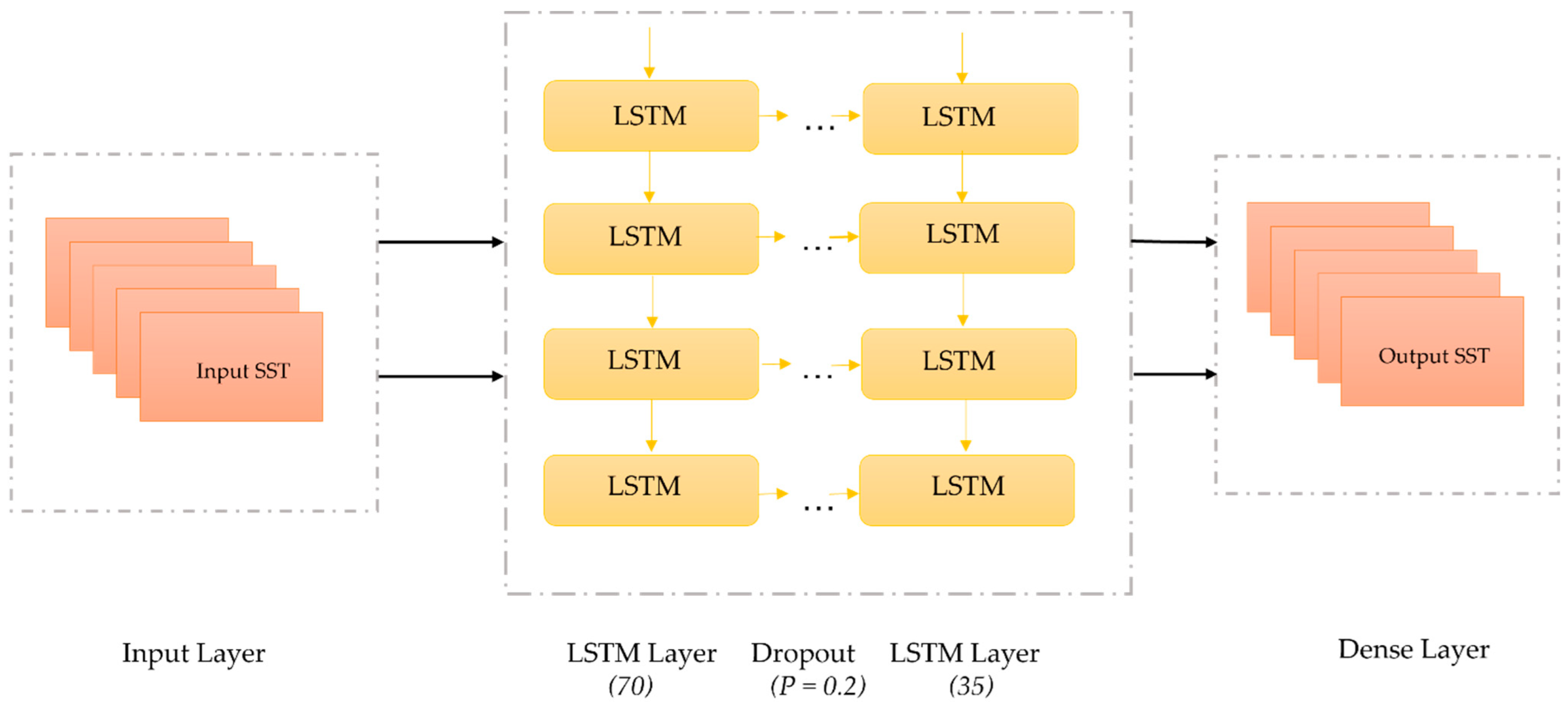
2.2.2. Model Building

This study constructed a 4-layer LSTM model based on Keras, including an input layer, two LSTM layers, and a dense layer, as shown in Figure 2. During the training process of the LSTM model, parameters, such as weight vector W and bias vector b, are updated by error back propagation. The updating methods mainly include stochastic gradient descent [52], AdaGrad, RMSProp [53], adaptive momentum estimation algorithms, and so on. Among them, the Adam optimization algorithm is an effective stochastic optimization algorithm based on gradient learning. The algorithm integrates the advantages of AdaGrad and RMSProp algorithm, has an adaptive learning rate for different parameters, and occupies fewer storage resources. Compared with other stochastic optimization algorithms, the Adam algorithm performs better in practical applications [54]. Therefore, the Adam optimization algorithm is adopted in this study.

Suppose the time series of SST is expressed as $X=X_t$, $t=1,2,3\cdots n$, where $X_t$ is the SST at time t. Given the window length of the neural network, this parameter indicates that SST at the next moment, which is described $P_{t+L}$, is predicted using the historical SST with the time length of L, which is represented as $X_t, X_{t+1}\cdots X_{t+L-1}$. The prediction steps of SST are as follows:

(1)

Network initialization. Weights vector W and bias vector b are randomly initialized. The initial learning rate and the maximum number of iterations are set to 0.0001 and 100, respectively, where EarlyStopping is used in the number of iterations.

(2)

Data standardization. The missing values in the data are filled with the surrounding values, and the MinmaxScaler function is imported from the sklearn library to standardize the dataset X to (−1, 1) to obtain the standardized dataset X.

(3)

The division of dataset X. The standardized dataset X is set according to the window length L and the number of days of prediction, in which the training set and the validation set are divided into 85% and 15%, respectively.

(4)

Error calculation. The error between the output of the output layer and the satellite data and the loss function are calculated using MSE.

(5)

Update of weights and thresholds. Using the Adam gradient optimization algorithm, update the weights W and biases b according to the loss function.

(6)

Repeat steps (3) to (5). The training ends when the training times reach the maximum number of iterations, or the value of the loss function does not change for three consecutive iterations.

2.2.3. Evaluation Indicators

To evaluate the prediction performance of SST, the predicted SST is compared with OSTIA data using the coefficient of determination ($R^2$), root mean square error (RMSE), and absolute error (AE). The formula is as follows:

$$R^2=1-\frac{{\sum }_{i=1}^m{\left(ss{t}_o-ss{t}_p\right)}^2}{{\sum }_{i=1}^m{\left(ss{t}_o-\overline{ss{t}_o}\right)}^2}$$

(7)

$$RMSE=\sqrt{\frac{1}{m}{{\displaystyle \sum }}_{i=1}^m{\left(ss{t}_o-ss{t}_p\right)}^2}$$

(8)

$$AE=\left|ss{t}_o-ss{t}_p\right|$$

(9)

$$Improve rate=\frac{A{E}_{max}-A{E}_{min}}{A{E}_{max}}$$

(10)

where $ss{t}_{o }$ and $ss{t}_p$ are OSTIA value and predicted value of SST, and m is the total number of samples. The smaller the RMSE and AE, the more accurate the prediction, and the closer $R^2$ value is to 1, the higher the fit between the predicted and true values. $A{E}_{max}$ is the maximum value of each column of AE, $A{E}_{min}$ is the minimum value of each column of AE.

3. Results

SST of the ECS varies greatly from nearshore to far sea, and the ocean current also greatly impacts the sea surface temperature change in this area. Therefore, according to the above reasons, the four points, L1 (31.5°N, 122°E), L2 (25.5°N, 122.5°E), L3 (24.5°N,128°E), and L4 (30.5°N, 129.2°E) as shown in Figure 3, are selected to analyze the sea surface temperature predicted by the LSTM model. The reasons for selecting these four points are as follows: (1) The seasonal variation in the Yangtze River estuary area is very obvious, and SST varies greatly, with a minimum value of approximately 7 °C and a maximum value of approximately 30 °C. Therefore, L1 is selected near the Yangtze River estuary; (2) The Kuroshio is a powerful western boundary warm current in the northwestern Pacific Ocean. It has obvious characteristics, such as fast speed, narrow flow width, large flow, high temperature, and high salinity [55,56], which have an important impact on China’s climate. Therefore, to analyze the change of SST in the Kuroshio area, L2 and L3 with different water depths on both sides of the Kuroshio are selected to represent Kuroshio; (3) Compared with the other three points, the water depth value of L4 is larger than 7000 m. Thus, L3 is selected at the position shown in Figure 3.

3.1. The Effect of Different Parameter Settings on LSTM Prediction Performance

The prediction performance of the LSTM model is affected by parameter settings. For example, learning rate, the number of network layers, the input length, and the prediction length will all affect the prediction effect. However, this subsection mainly explores the influence of input length and prediction length on the prediction performance of LSTM models through RMSE, AE, and $R^2$.

3.1.1. The Impact of Input Length on LSTM Prediction Performance

In order to verify the influence of input length on the prediction results of the model, under the condition that hyperparameters, such as the learning rate, the number of hidden layers, and the number of neurons, do not change, the prediction length is controlled to 5, and the input length is set to 2, 5, 10, and 15 days, respectively, to discuss the impact of input length changes. The influence of input length on the prediction of the LSTM model is shown in

Table 1. RMSE (°C) variation of different input lengths at different positions, where the bold font is the minimum value of each column.

	Location	L1	L2	L3	L4
Length of Input
2		0.3465	0.2698	0.1786	0.3331
5		0.2741	0.0568	0.0458	0.0769
10		0.2730	0.0917	0.0707	0.0764
15		0.2461	0.0995	0.1005	0.0698

,

Table 2. $R^2$ variation of different input lengths at different positions, where the bold font is the maximum value of each column.

	Location	L1	L2	L3	L4
Length of Input
2		0.9976	0.9830	0.9949	0.9884
5		0.9985	0.9992	0.9996	0.9993
10		0.9985	0.9980	0.9992	0.9994
15		0.9988	0.9977	0.9984	0.9995

and

Table 3. AE (°C) variation of different input lengths at different positions, where the bold font is the minimum value of each column.

	Location	L1		L2		L3		L4
Length of Input		Max	Mean	Max	Mean	Max	Mean	Max	Mean
2		1.3978	0.2454	0.9512	0.1979	0.7163	0.1356	1.1755	0.2471
5		1.1656	0.1968	0.2773	0.0406	0.1893	0.0328	0.3873	0.0574
10		1.0081	0.2003	0.5757	0.0634	0.2271	0.0540	0.3401	0.0551
15		0.8816	0.1833	0.5338	0.0724	0.3605	0.0773	0.3624	0.0500
Improve Rate		36.93%	25.31%	70.85%	79.48%	73.57%	75.81%	71.07%	79.77%

, where the bold font is the extremum value of each column. It is worth noting that, compared with other input lengths, when the input length is 2, the RMSE and AE at the four positions are the maximum value and $R^2$ is the minimum. Then, with the increase of the input length, the RMSE and AE decreases significantly and $R^2$ increases compared with the input length of 2. Especially when the input length is 5, the RMSE and AE values of L2 and L3 positions are the smallest, and when the input length is 15, the RMSE values of L1 and L4 positions are the smallest. Moreover, $R^2$also becomes larger at the corresponding positions above. This proves that if the input length is too small, the LSTM model cannot capture the change law of the SST data well. Increasing the input length can improve the prediction performance of the LSTM model to a certain extent. However, no obvious positive correlation is seen between them. In fact, the improvement of the prediction performance of the LSTM model is not only related to the input length, but also related to the predicted position. The selection of appropriate input length should consider related factors, such as the predicted position.

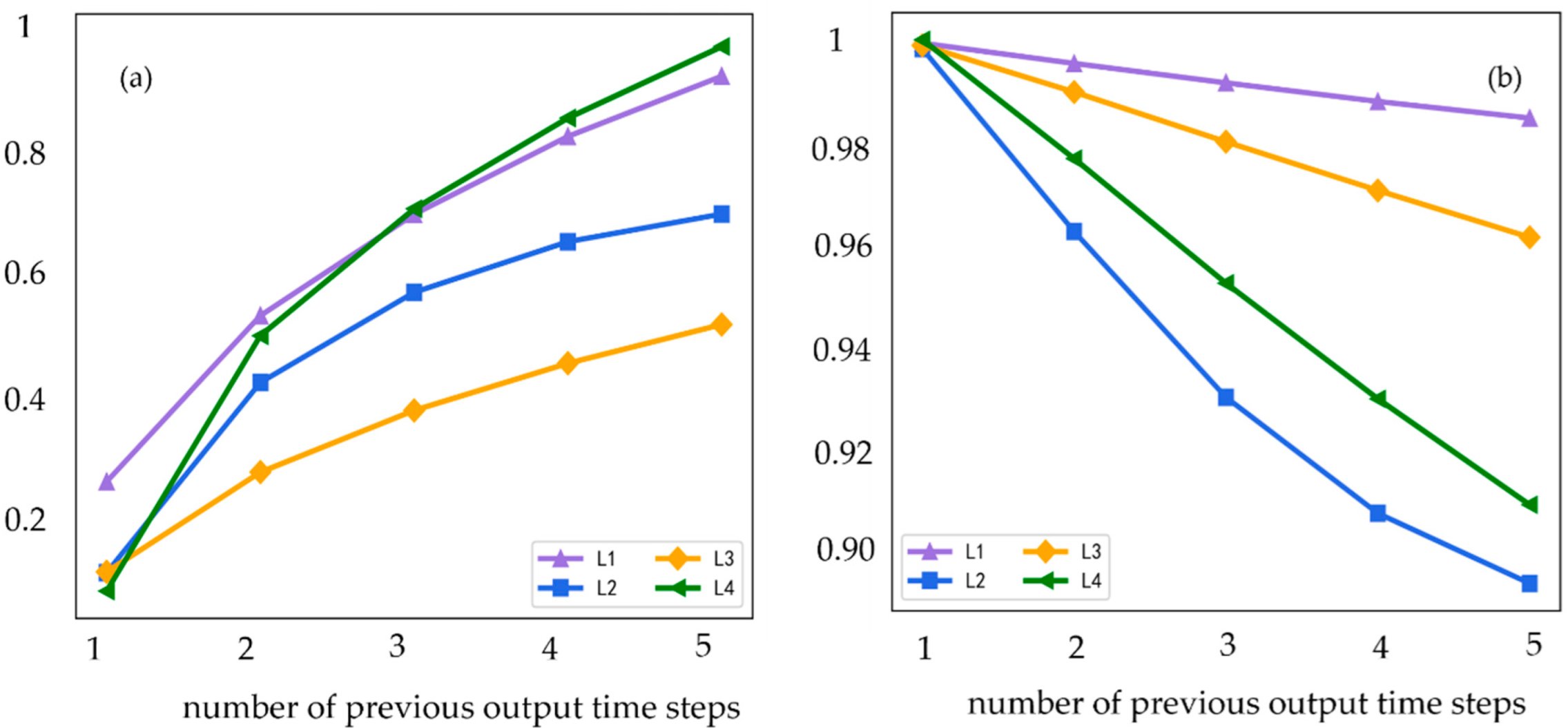
3.1.2. The Impact of Prediction Lengths on LSTM Prediction Performance

Similarly, to explore the influence of the prediction length on the prediction results of the model, when the other hyperparameters mentioned above remain unchanged, the input length is controlled to 15 in combination with Table 1 and Table 2. The main reason is that, when the input length is set to 5, the input length may be short, and the data change law may not be well displayed. Furthermore, L1 has the largest difference in the extremum among the four positions, so the change law of the SST data is the most difficult to capture. When the input length is 15, the RMSE is the smallest and $R^2$ is the largest in L1, and the LSTM model has the best prediction effect. To sum up, this paper believes that it is better to set the input length to 15. Figure 4 shows the RMSE and $R^2$ values for 5 prediction steps, where the different colors of the lines represent each specific location. We can see that when the prediction length is 1, the RMSE value is the minimum value at any position, and the $R^2$ value is the maximum value. When the prediction length is 5, the RMSE at any position is the maximum value, and the $R^2$ is the minimum value, that is, the minimum value of RMSE and the maximum value of $R^2$ are obtained almost at the same time. Meanwhile, it also shows that the prediction performance of the LSTM model decreases gradually with the increase of prediction length.

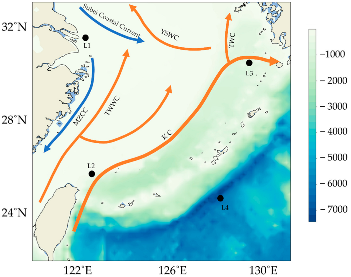
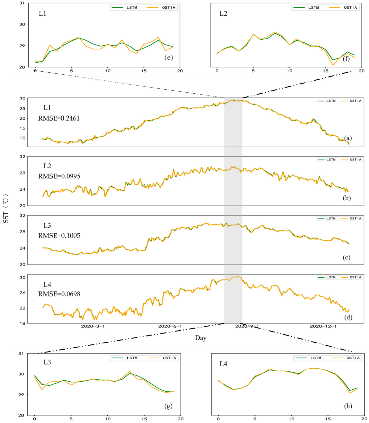
3.2. Analysis of Prediction Results at Different Points

In order to analyze the variation trend of the LSTM model prediction results and error over time at different locations, Figure 5 and Figure 6 are drawn. Meanwhile, to explore the accuracy of the LSTM model for extreme value prediction, we selected the region with the largest SST in a year, as shown in the gray rectangle in Figure 5. According to (a)–(d) of Figure 5, we found that the prediction results of the LSTM model for L1, L2, L3, and L4 are slightly different from OSTIA, and cyclical trends are represented accurately. However, from Figure 5e–g, it is found that the LSTM model is not very accurate in predicting extremum. In Figure 5h, it is found that LSTM is quite accurate for predicting extremum. The reason is that the RMSE value here is particularly small. That is, except that the RMSE value is particularly small, the LSTM model cannot predict the extremum well in most cases. According to Figure 6, it is found that the difference between the prediction results of the LSTM model and the OSTIA data changes greatly at the L1 position. The maximum value of the difference between the two is 0.7 °C and the minimum value is −0.9 °C. At the L4 position, their differences are relatively small and stable, and most of the differences are −0.1 °C. Furthermore, the maximum value of RMSE at L1 position is 0.2461 °C, and the minimum value of RMSE at L4 position is 0.0698 °C. The large difference between L1 and L4 is mainly because L1 is located at the estuary of the Yangtze River. The seasonal variation of SST at the estuary of the Yangtze River is more obvious, so that the LSTM model cannot capture the SST law of L1 position well. Moreover, the RMSE value of the L4 position is smaller than that of the L3 position, which may be due to the lower water depth of the L3 position than that of the L4 position.

3.3. Migration Analysis

This subsection mainly describes the feasibility of applying the L4 position trained model to the prediction of SST in ECS from the following two aspects: (1) Study its migration from the spatial distributions of RMSE and AE of each month as shown in Figure 7, Figure 8 and Figure 9. (2) Due to the obvious seasonal variation of SST, the spatial distributions of RMSE and AE of four seasons are described to verify its migration as shown in Figure 10 and Figure 11.

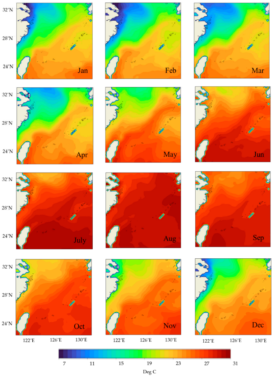
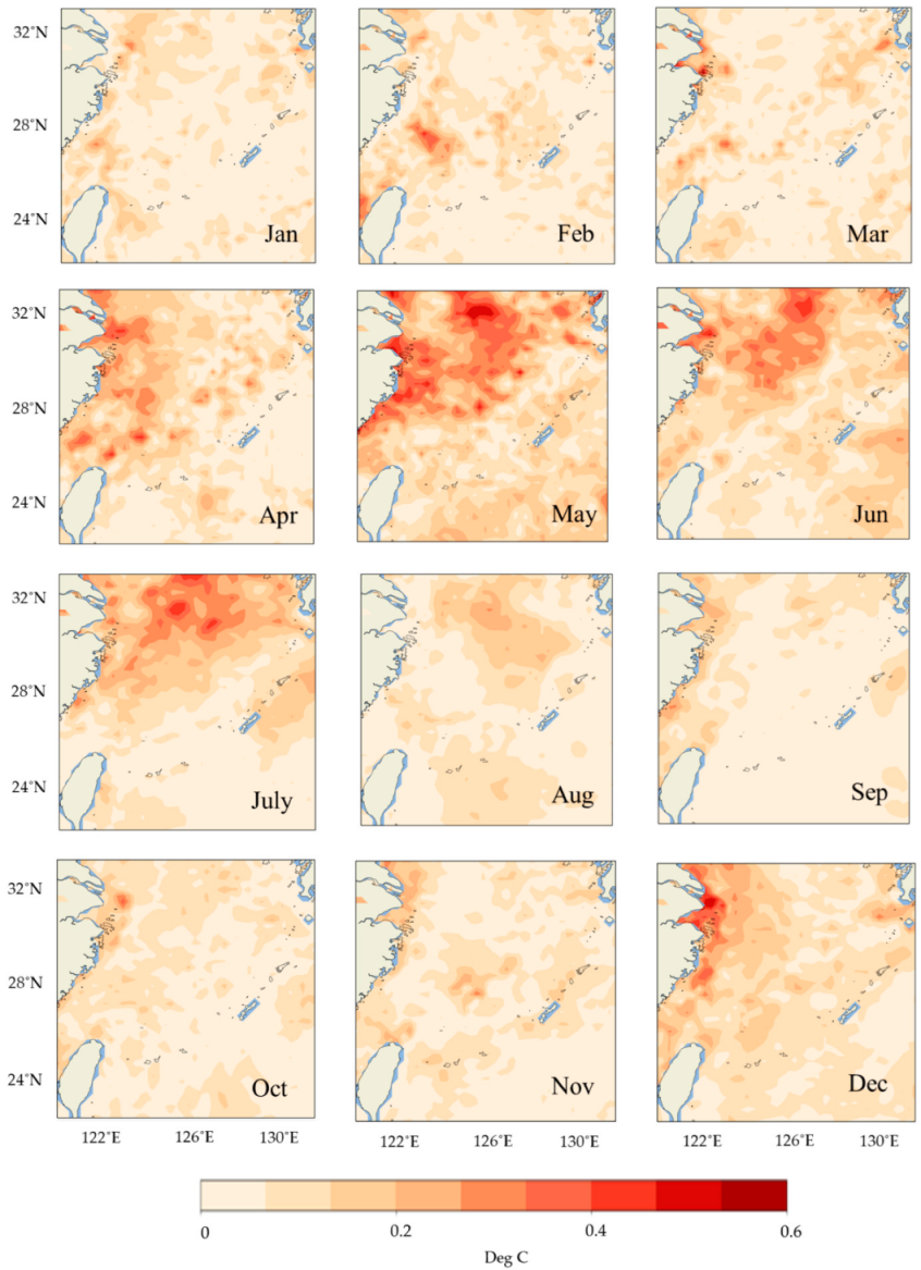
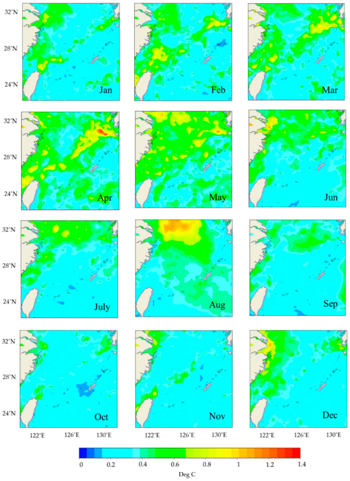
3.3.1. Migration Analysis for Monthly Changes

Given that the RMSE value of the L4 position in Figure 5 is the smallest, the LSTM model trained at the L4 position is selected to predict the SST of the whole study area in 2020 to prove whether the LSTM network has the characteristics of migration. The spatial distribution of SST in 2020 predicted by the LSTM model is shown in Figure 7. The characteristics of SST, such as the Kuroshio, the Min-Zhe coastal current, and the Yangtze River Diluting Water, are clearly displayed in the forecast map and show obvious seasonal changes. For the quality evaluation of LSTM prediction results, the methods of AE and RMSE are used. Figure 8 presents the AE between the prediction results of the model and the OSTIA satellite data in 2020. We can see that the error between the prediction results and OSTIA are mostly less than 0.4 °C, and the AE of the Yangtze River estuary and its northern part and Min-Zhe coastal currents is relatively large in April, May, June, July, and December. Figure 9 shows that most of the RMSE values in 2020 are less than 0.5 °C. In April, maximum RMSE is found around the Kuroshio and TWC area, that is, the dispersion of error in this region is relatively large. In August, the error dispersion in the northern part of the Yangtze River estuary is relatively high. In general, the areas with higher error dispersion in a year are located in the Yangtze River estuary and its north, the Kuroshio, and the Min-Zhe coastal current.

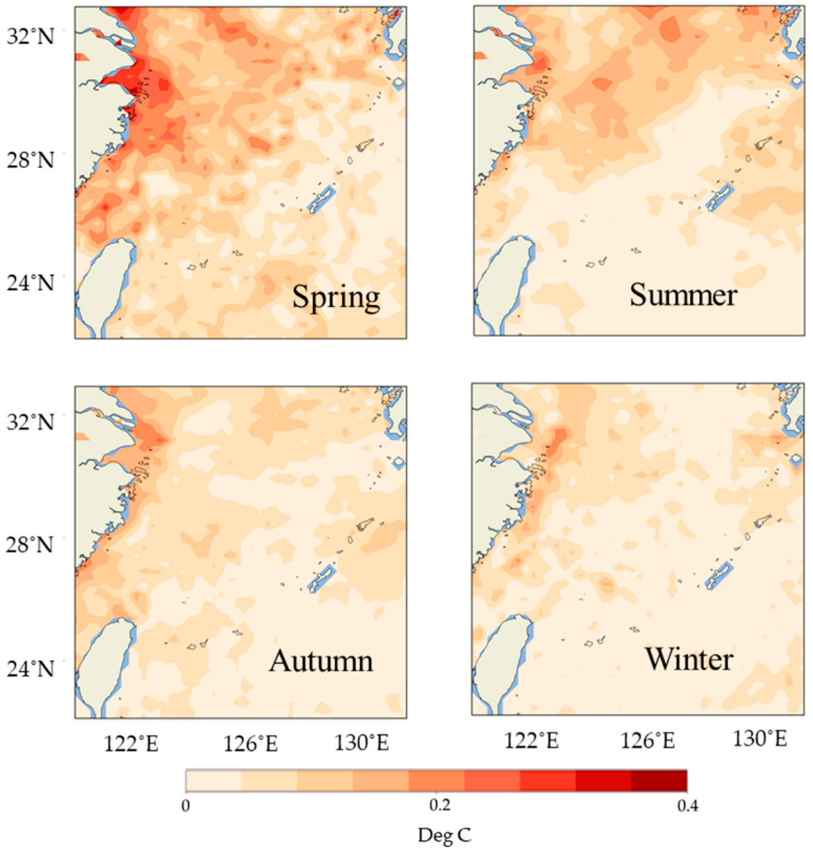
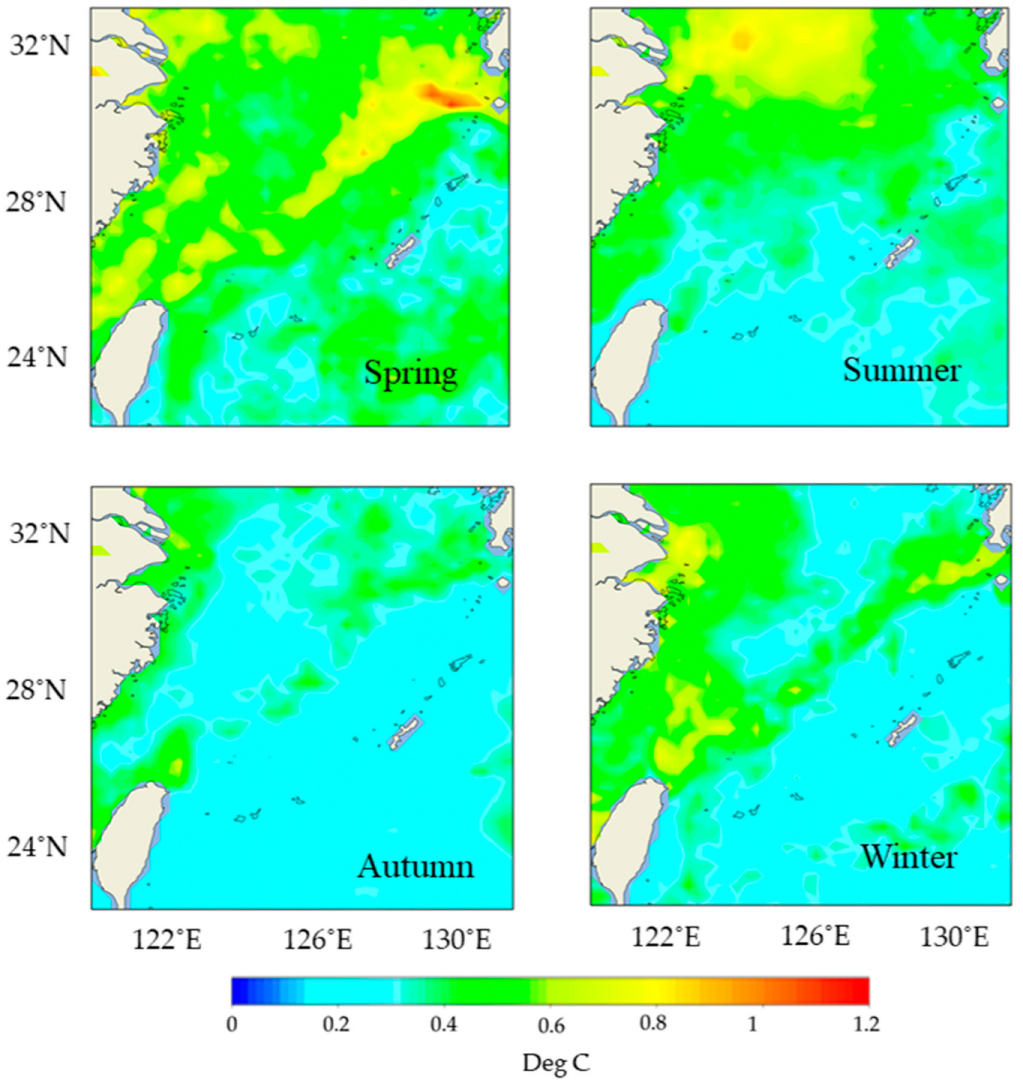
3.3.2. Mobility Analysis of Seasonal Changes

Figure 10 is drawn for the seasonal AE in spring, summer, autumn, and winter to analyze whether the migration of the LSTM model in ECS can show the characteristics of seasonal changes well. AE between the predicted results of the LSTM model and OSTIA, shown in Figure 10, is within 0.4 °C, and the maximum value of AE decreases by 0.2 °C compared with Figure 8. Among the four seasons, AE of spring is the largest, and AE of autumn and winter is smaller. Moreover, the extremum of AE of the four seasons is mainly concentrated in the area of the Yangtze River Estuary and the Min-Zhe coastal current. Through the analysis of the dispersion degree of the error in Figure 11, the RMSE of the Kuroshio in spring is larger than that in other seasons, which means that the dispersion degree of errors in this area is large. In summer, the dispersion degree of error is large in the north of the Yangtze River Estuary. Through the analysis of AE and RMSE of each month and four seasons, the maximum value of AE and RMSE are 0.4 °C in four seasons, which is 0.2 °C lower than each month. However, most AE and RMSE values are relatively small, which are less than 0.4 °C and 0.5 °C, respectively. Therefore, the long-term and seasonal change law can be well represented by the migration of the LSTM model.

4. Conclusions

The past research at home and abroad has used many related SST prediction methods, such as numerical simulation, BP neural network, etc. In this study, the LSTM neural network is applied to the SST prediction, and its feasibility is discussed. The most important findings of this study are as follows:

(1)

The input and prediction lengths will affect the prediction performance of the LSTM model. The increase of the input length can improve the prediction performance of the LSTM model to a certain extent, but no obvious positive correlation is seen between them. Meanwhile, the prediction performance of the LSTM model decreases with the increase of the prediction length, and an obvious negative correlation is seen between them. The effect is the best when the prediction length is 1 and the worst when it is 5.

(2)

The prediction results of the LSTM model for a single site are quite accurate, but the extremum cannot be well displayed. Furthermore, affected by the seasonal variation of the Yangtze River Estuary, the prediction result of the Yangtze River Estuary site is the worst compared with other regions.

(3)

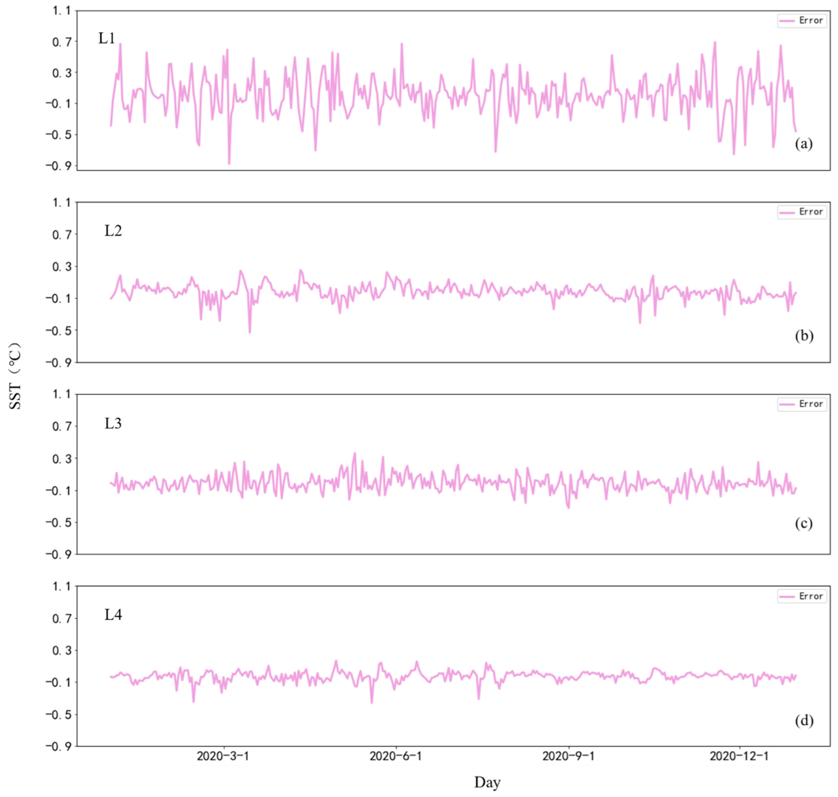
By analyzing the AE and RMSE of the prediction results of the LSTM model, most of the error is found to be less than 0.4 °C and 0.5 °C, respectively, and the LSTM model has a very successful migration in the East China Sea. In addition, the AE and RMSE of the seasonal and monthly average have prominent spatial characteristics. The places with larger error are distributed in the Yangtze River estuary and its north, the Kuroshio, and the Min-Zhe coastal current.

Using the LSTM neural network to predict SST is a new prediction method, which has achieved good results in the experiment of SST prediction. Therefore, it can be a better tool and method to predict the change in SST. However, the interpretability of deep learning remains a hot issue in the computer field. Explaining the LSTM network’s physical mechanism more effectively for predicting SST still needs further experimental research.

References

1. Sumner, M.D.; Michael, K.J.; Bradshaw, C.J.A.; Hindell, M.A. Remote sensing of Southern Ocean sea surface temperature: Implications for marine biophysical models. Remote Sens. Environ. 2003, 84, 161–173. [Google Scholar] [CrossRef]
2. Wentz, F.J.; Gentemann, C.; Smith, D.; Chelton, D. Satellite Measurements of Sea Surface Temperature through Clouds. Science 2000, 288, 847–850. [Google Scholar] [CrossRef] [PubMed] [Green Version]
3. Rauscher, S.A.; Jiang, X.; Steiner, A.; Williams, A.P.; Jiang, X. Sea Surface Temperature Warming Patterns and Future Vegetation Change. J. Clim. 2015, 28, 7943–7961. [Google Scholar] [CrossRef] [Green Version]
4. Salles, R.; Mattos, P.; Iorgulescu, A.-M.D.; Bezerra, E.; Lima, L.; Ogasawara, E. Evaluating temporal aggregation for predicting the sea surface temperature of the Atlantic Ocean. Ecol. Inform. 2016, 36, 94–105. [Google Scholar] [CrossRef]
5. Bouali, M.; Sato, O.T.; Polito, P.S. Temporal trends in sea surface temperature gradients in the South Atlantic Ocean. Remote Sens. Environ. 2017, 194, 100–114. [Google Scholar] [CrossRef]
6. Cane, M.A.; Kaplan, A.; Clement, A.C.; Kushnir, Y. Twentieth-Century Sea Surface Temperature Trends. Science 1997, 275, 957–960. [Google Scholar] [CrossRef] [Green Version]
7. Castro, S.L.; Wick, G.A.; Steele, M. Validation of satellite sea surface temperature analyses in the Beaufort Sea using UpTempO buoys. Remote Sens. Environ. 2016, 187, 458–475. [Google Scholar] [CrossRef]
8. Chaidez, V.; Dreano, D.; Agusti, S.; Duarte, C.M.; Hoteit, I. Decadal trends in Red Sea maximum surface temperature. Sci. Rep. 2017, 7, 8144. [Google Scholar] [CrossRef] [Green Version]
9. Herbert, T.D.; Peterson, L.C.; Lawrence, K.T.; Liu, Z. Tropical ocean temperatures over the past 3.5 million years. Science 2010, 328, 1530–1534. [Google Scholar] [CrossRef]
10. Yao, S.; Luo, J.; Huang, G.; Wang, P. Distinct global warming rates tied to multiple ocean surface temperature changes. Nat. Clim. Change 2017, 7, 486–491. [Google Scholar] [CrossRef]
11. Jiao, N.; Zhang, Y.; Zeng, Y.; Gardner, W.D. Ecological anomalies in the East China Sea: Impacts of the Three Gorges Dam? Water Res. 2007, 41, 1287–1293. [Google Scholar] [CrossRef] [PubMed]
12. Du, B.; Yuan, X. Analysis and Forecast of Sea Surface Temperature Field for the East China Sea and the adjacent waters. Mar. Forecast. 1986, 1, 3–11. [Google Scholar]
13. Gao, G.; Marin, M.; Feng, M.; Yin, B.; Yang, D.; Feng, X.; Ding, Y.; Song, D. Drivers of Marine Heatwaves in the East China Sea and the South Yellow Sea in Three Consecutive Summers During 2016–2018. J. Geophys. Res. Ocean. 2020, 125, e16518. [Google Scholar] [CrossRef]
14. Tiwari, P.; Dimri, A.P.; Shenoi, S.C.; Francis, P.A.; Jithin, A.K. Impact of Surface forcing on simulating Sea Surface Temperature in the Indian Ocean—A study using Regional Ocean Modeling System (ROMS). Dyn. Atmos. Ocean. 2021, 95, 101243. [Google Scholar] [CrossRef]
15. Gao, S.; Lv, X.; Wang, H. Sea Surface Temperature Simulation of Tropical and North Pacific Basins Using a Hybrid Coordinate Ocean Model (HYCOM). Mar. Sci. Bull. 2008, 10, 1–14. [Google Scholar]
16. Arx, W. An Introduction to Physical Oceanography. Am. J. Phys. 2005, 30, 775–776. [Google Scholar] [CrossRef]
17. Bell, M.J.; Schiller, A.; Le Traon, P.Y. An introduction to GODAE OceanView. J. Oper. Oceanogr. 2015, 8 (Suppl. 1), s2–s11. [Google Scholar] [CrossRef]
18. Xue, Y.; Leetmaa, A. Forecasts of tropical Pacific SST and sea level using a Markov model. Geophys. Res. Lett. 2000, 27, 2701–2704. [Google Scholar] [CrossRef] [Green Version]
19. Laepple, T.; Jewson, S. Five year ahead prediction of Sea Surface Temperature in the Tropical Atlantic: A comparison between IPCC climate models and simple statistical methods. arXiv 2007, arXiv:physics/0701165. [Google Scholar] [CrossRef]
20. Collins, D.C.; Reason, C.; Tangang, F. Predictability of Indian Ocean sea surface temperature using canonical correlation analysis. Clim. Dyn. 2004, 22, 481–497. [Google Scholar] [CrossRef]
21. Peng, Y.; Wang, Q.; Yuan, C.; Lin, K. Review of Research on Data Mining in Application of Meteorological Forecasting. J. Arid. Meteorol. 2015, 33, 9. [Google Scholar]
22. Kusiak, A.; Zheng, H.; Song, Z. Wind farm power prediction: A data-mining approach. Wind Energy 2009, 12, 275–293. [Google Scholar] [CrossRef]
23. Ho, H.C.; Knudby, A.; Sirovyak, P.; Xu, Y.; Hodul, M. Mapping maximum urban air temperature on hot summer days. Remote Sens. Environ. 2014, 154, 38–45. [Google Scholar] [CrossRef]
24. Behrang, M.A.; Assareh, E.; Ghanbarzadeh, A.; Noghrehabadib, A.R. The potential of different artificial neural network (ANN) techniques in daily global solar radiation modeling based on meteorological data. Sol. Energy 2010, 84, 1468–1480. [Google Scholar] [CrossRef]
25. Mellit, A.; Pavan, A.M.; Benghanem, M. Least squares support vector machine for short-term prediction of meteorological time series. Theor. Appl. Climatol. 2012, 111, 297–307. [Google Scholar] [CrossRef]
26. Yue, L.; Shen, H.; Zhang, L.; Zheng, X.; Zhang, F.; Yuan, Q. High-quality seamless DEM generation blending SRTM-1, ASTER GDEM v2 and ICESat/GLAS observations. ISPRS J. Photogramm. Remote Sens. 2017, 123, 20–34. [Google Scholar] [CrossRef] [Green Version]
27. Zang, L.; Mao, F.; Guo, J.; Wang, W.; Pan, Z.; Shen, H.; Zhu, B.; Wang, Z. Estimation of spatiotemporal PM 1.0 distributions in China by combining PM 2.5 observations with satellite aerosol optical depth. Sci. Total Environ. 2019, 658, 1256–1264. [Google Scholar] [CrossRef]
28. Tangang, F.T.; Tang, B.; Monahan, A.H. Forecasting ENSO Events: A Neural Network–Extended EOF Approach. J. Clim. 1998, 11, 29–41. [Google Scholar] [CrossRef]
29. Tangang, F.T.; Hsieh, W.W.; Tang, B.; Hsieh, W.W. Forecasting the equatorial Pacific sea surface temperatures by neural network models. Clim. Dyn. 1997, 13, 135–147. [Google Scholar] [CrossRef]
30. Tangang, F.T.; Hsieh, W.W.; Tang, B. Forecasting regional sea surface temperatures in the tropical Pacific by neural network models, with wind stress and sea level pressure as predictors. J. Geophys. Res. Ocean. 1998, 103, 7511–7522. [Google Scholar] [CrossRef]
31. Wu, A.; Hsieh, W.W.; Tang, B. Neural network forecasts of the tropical Pacific sea surface temperatures. Neural Netw. 2006, 19, 145–154. [Google Scholar] [CrossRef] [Green Version]
32. Gupta, S.M.; Malmgren, B.A. Comparison of the accuracy of SST estimates by artificial neural networks (ANN) and other quantitative methods using radiolarian data from the Antarctic and Pacific Oceans. Earth Sci. India 2009, 2, 52–75. [Google Scholar]
33. Tripathi, K.C.; Das, I.; Sahai, A.K. Predictability of sea surface temperature anomalies in the Indian Ocean using artificial neural networks. Indian J. Mar. Sci. 2006, 35, 210–220. [Google Scholar]
34. Patil, K.; Deo, M.C.; Ghosh, S.; Ravichandran, M. Predicting Sea Surface Temperatures in the North Indian Ocean with Nonlinear Autoregressive Neural Networks. Int. J. Oceanogr. 2013, 2013, 302479. [Google Scholar] [CrossRef] [Green Version]
35. Patil, K.; Deo, M.C. Prediction of daily sea surface temperature using efficient neural networks. Ocean. Dyn. 2017, 67, 357–368. [Google Scholar] [CrossRef]
36. Mahongo, S.B.; Deo, M.C. Using Artificial Neural Networks to Forecast Monthly and Seasonal Sea Surface Temperature Anomalies in the Western Indian Ocean. Int. J. Ocean. Clim. Syst. 2013, 4, 133–150. [Google Scholar] [CrossRef] [Green Version]
37. Aparna, S.G.; D’Souza, S.; Arjun, N.B. Prediction of daily sea surface temperature using artificial neural networks. Int. J. Remote Sens. 2018, 39, 4214–4231. [Google Scholar] [CrossRef]
38. Hou, S.; Li, W.; Liu, T.; Zhou, S.; Guan, J.; Qin, R.; Wang, Z. MIMO: A Unified Spatio-Temporal Model for Multi-Scale Sea Surface Temperature Prediction. Remote Sens. 2022, 14, 2371. [Google Scholar] [CrossRef]
39. Lecun, Y.; Bengio, Y.; Hinton, G. Deep learning. Nature 2015, 521, 436. [Google Scholar] [CrossRef]
40. Zhang, Q.; Wang, H.; Dong, J.; Zhong, G.; Sun, X. Prediction of Sea Surface Temperature Using Long Short-Term Memory. IEEE Geosci. Remote Sens. Lett. 2017, 14, 1745–1749. [Google Scholar] [CrossRef] [Green Version]
41. Sarkar, P.P.; Janardhan, P.; Roy, P. Prediction of sea surface temperatures using deep learning neural networks. SN Appl. Sci. 2020, 2, 1458. [Google Scholar] [CrossRef]
42. Kim, M.; Yang, H.; Kim, J. Sea Surface Temperature and High Water Temperature Occurrence Prediction Using a Long Short-Term Memory Model. Remote Sens. 2020, 12, 3654. [Google Scholar] [CrossRef]
43. Li, X. Sea surface temperature prediction model based on long and short-term memory neural network. IOP Conf. Ser. Earth Environ. Sci. 2021, 658, 12040. [Google Scholar] [CrossRef]
44. Xiao, C.; Chen, N.; Hu, C.; Wang, K. Short and mid-term sea surface temperature prediction using time-series satellite data and LSTM-AdaBoost combination approach. Remote Sens. Environ. 2019, 233, 111358. [Google Scholar] [CrossRef]
45. Xiao, C.; Chen, N.; Hu, C.; Wang, K. A spatiotemporal deep learning model for sea surface temperature field prediction using time-series satellite data. Environ. Model. Softw. 2019, 120, 104501–104502. [Google Scholar] [CrossRef]
46. Wei, L.; Guan, L.; Qu, L.; Guo, D. Prediction of Sea Surface Temperature in the China Seas Based on Long Short-Term Memory Neural Networks. Remote Sens. 2020, 12, 2697. [Google Scholar] [CrossRef]
47. Sun, Y.; Yao, X.; Bi, X.; Huang, X.; Zhao, X.; Qiao, B. Time-Series Graph Network for Sea Surface Temperature Prediction. Big Data Res. 2021, 25, 100237. [Google Scholar] [CrossRef]
48. Zhang, Z.; Pan, X.; Jiang, T.; Sui, B.; Liu, C.; Sun, W. Monthly and Quarterly Sea Surface Temperature Prediction Based on Gated Recurrent Unit Neural Network. J. Mar. Sci. Eng. 2020, 8, 249. [Google Scholar] [CrossRef] [Green Version]
49. Donlon, C.J.; Martin, M.; Stark, J. Roberts-Jones, J.; Fiedler, E.; Wimmer, W. The Operational Sea Surface Temperature and Sea Ice Analysis (OSTIA) system. Remote Sens. Environ. 2012, 116, 140–158. [Google Scholar] [CrossRef]
50. Jiang, X.; Xi, M.; Song, Q. A comparison analysis of six sea surface temperature products. Acta Oceanol. Sin. 2013, 35, 88–97. [Google Scholar]
51. Hochreiter, S.; Schmidhuber, J. Long Short-Term Memory. Neural Comput. 1997, 9, 1735–1780. [Google Scholar] [CrossRef] [PubMed]
52. Graves, A.; Schmidhuber, J. Framewise phoneme classification with bidirectional LSTM and other neural network architectures. Neural Netw. 2005, 18, 602–610. [Google Scholar] [CrossRef] [PubMed]
53. Duchi, J.; Hazan, E.; Singer, Y. Adaptive Subgradient Methods for Online Learning and Stochastic Optimization. J. Mach. Learn. Res. 2011, 12, 2121–2159. [Google Scholar]
54. Kingma, D.P.; Ba, J. Adam: A Method for Stochastic Optimization. arXiv 2014, arXiv:1412.6980. [Google Scholar] [CrossRef]
55. Su, J.L.; Guan, B.X.; Jiang, J.Z. The Kuroshio. Part I. Physical features. Oceanogr. Mar. Biol. Annu. Rev. 1990, 28, 11–71. [Google Scholar]
56. Bryden, H.L.; Roemmich, D.H.; Church, J.A. Ocean heat transport across 24°N in the Pacific. Deep Sea Res. 1991, 38, 297–324. [Google Scholar] [CrossRef]
Figure 1. Structure of long short-term memory (LSTM) memory cell, including the forget, input, and output gates.
Remotesensing 14 03300 g001
Figure 2. The architecture of the proposed LSTM deep neural network for SST prediction.
Remotesensing 14 03300 g002
Figure 3. Location diagram of different points. The black dots represent the selected positions. MZCC, TWWC, YSWC, TWC, and KC represent the Min-Zhe Costal Current (Min is Fujian province, Zhe is Zhejiang Province), the Taiwan Warm Current, the Yellow Sea Warm Current, the Tsushima Warm Current, and the Kuroshio, respectively. Besides the blue line is the cold current, and the red line is the warm current and the unit of colorbar is meters.
Remotesensing 14 03300 g003
Figure 4. RMSE (°C) and R 2 of different prediction lengths at different positions, where lines with different colors represent different positions, (a) RMSE at different positions, (b) R 2 at different positions, the abscissa is the number of days predicted in advance.
Remotesensing 14 03300 g004
Figure 5. OSTIA data and LSTM predictions at different points, where the green line is the prediction result of LSTM, the yellow line is the OSTIA data, and the gray rectangle is the area where the maximum SST is located in 2020. (ad) are in a comparison chart of the LSTM prediction results and OSTIA data in 2020. (eh) are the values of the region where the maximum SST is located in 2020. The abscissa is the SST in degrees Celsius, and the ordinate is the number of days.
Remotesensing 14 03300 g005
Figure 6. The error of OSTIA data and LSTM prediction results at different points, where the error is obtained by subtracting the OSTIA data and the LSTM prediction result. (ad) are the errors of L1, L2, L3 and L4, respectively. The abscissa is SST in degrees Celsius, and the ordinate is the number of days.
Remotesensing 14 03300 g006
Figure 7. Spatial distribution of monthly mean sea surface temperature predicted by LSTM model in 2020, the unit of colorbar is degrees Celsius.
Remotesensing 14 03300 g007
Figure 8. Spatial distribution of monthly mean AE of OSTIA data and LSTM predictions of sea surface temperature in 2020. The unit of colorbar is degrees Celsius.
Remotesensing 14 03300 g008
Figure 9. Spatial distribution of monthly mean RMSE between LSTM predicted sea surface temperature and OSTIA data in 2020. The unit of colorbar is degrees Celsius.
Remotesensing 14 03300 g009
Figure 10. Spatial distribution of AE of OSTIA data and LSTM predictions of SST in four seasons, in which spring is from March to May, summer is from June to August, autumn is from September to November, and winter is from December to February. The unit of colorbar is degrees Celsius.
Remotesensing 14 03300 g010
Figure 11. Spatial distribution of RMSE between LSTM predicted sea surface temperature and OSTIA data in four seasons, in which spring is from March to May, summer is from June to August, autumn is from September to November, and winter is from December to February. The unit of color bar is degrees Celsius.
Remotesensing 14 03300 g011