Interpreting Sentinel-1 SAR Backscatter Signals of Snowpack Surface Melt/Freeze, Warming, and Ripening, through Field Measurements and Physically-Based SnowModel

Abstract

The transition of a cold winter snowpack to one that is ripe and contributing to runoff is crucial to gauge for water resource management, but is highly variable in space and time. Snow surface melt/freeze cycles, associated with diurnal fluctuations in radiative inputs, are hallmarks of this transition. C-band synthetic aperture radar (SAR) reliably detects meltwater in the snowpack. Sentinel-1 (S1) C-band SAR offers consistent acquisition patterns that allow for diurnal investigations of melting snow. We used over 50 snow pit observations from 2020 in Grand Mesa, Colorado, USA, to track temperature and wetness in the snowpack as a function of depth and time during snowpack phases of warming, ripening, and runoff. We also ran the physically-based SnowModel, which provided a spatially and temporally continuous independent indication of snowpack conditions. Snowpack phases were identified and corroborated by comparing field measurements with SnowModel outputs. Knowledge of snowpack warming, ripening, and runoff phases was used to interpret diurnal changes in S1 backscatter values. Both field measurements and SnowModel simulations suggested that S1 SAR was not sensitive to the initial snowpack warming phase on Grand Mesa. In the ripening and runoff phases, the diurnal cycle in S1 SAR co-polarized backscatter was affected by both surface melt/freeze as well as the conditions of the snowpack underneath (ripening or ripe). The ripening phase was associated with significant increases in morning backscatter values, likely due to volume scattering from surface melt/freeze crusts, as well as significant decreases in evening backscatter values associated with snowmelt. During the runoff phase, both morning and evening backscatter decreased compared to reference values. These unique S1 diurnal signatures, and their interpretations using field measurements and SnowModel outputs, highlight the capacities and limitations of S1 SAR to understand snow surface states and bulk phases, which may offer runoff forecasting or energy balance model validation or parameterization, especially useful in remote or sparsely-gauged alpine basins.

1. Introduction and Background

Gauging the transition of a cold winter snowpack to one that is ripe and contributing to runoff underpins successful water resource management; it can vary substantially in space and time [1]. Accurately determining this transition is challenged by topographic and orographic complexity, spatial and temporal heterogeneity in snow precipitation as well as post-depositional processes, and sparse measurement in complex and varying mountainous terrain from which snowmelt often originates. Empirically-based runoff forecasting models that relate current conditions to the historical record are based on calibrated relationships that may not hold in a non-stationary climate. These methods are widely used in operational forecasting due to their simplicity and computational efficiency, but they do not incorporate all of the physical drivers and processes related to runoff; significant forecasting errors can result (e.g., [2,3]).

Field measurements offer indications of snowpack conditions that are discrete in space and time; while these measurements are typically accurate, they are often time- and labor-intensive, and are difficult to extrapolate to the catchment scale. Remotely sensed data offer a regional timestamp of snowpack conditions. A benefit of synthetic aperture radar (SAR) is the ability to image day or night and through cloud cover; the spatial resolution is often on the order of tens of meters, which allows for insight into some of the highly (spatially) variable snowpack processes. Additionally, C-band (about 5.5 cm wavelength) SAR is sensitive to the snowpack at multiple interfaces [4], which may be leveraged for understanding the energetic status of the snowpack. However, accurate interpretation of SAR snow signatures may require field validation and site-specific knowledge. Physically-based models mimic snow processes, offering a continuous (in space and time) indication of snowpack conditions; however, their performances are largely reliant on the quality of input data, and uncertainties from various sources (i.e., inputs, parameters, processes) proliferate to the results [5,6,7]. The integration of multiple observation modalities offers complementary perspectives on snowpack conditions and their potential drivers, which may also support anticipating changes in snowpack processes and runoff as climate changes.

In this study, we used snow pit observations from three related NASA SnowEx field campaigns during the winter and spring of 2020 in Grand Mesa, Colorado, to track temperature and wetness in the snowpack with depth and time. We used these field measurements to compare with physically-based SnowModel outputs of snow conditions in order to identify snowpack phases of warming, ripening, and runoff. Knowledge of these snowpack phases was then used to interpret diurnal changes in Sentinel-1 (S1) SAR backscatter values for the same timeframe. This interpretation highlights the capacities and limitations of S1 diurnal SAR to identify snow surface states and bulk phases remotely, which may provide spatially explicit information on snow conditions with which to compare, validate, or parameterize runoff forecasting or energy balance models, especially useful in remote or sparsely gauged terrain.

After providing background information for snowpack seasonal transitions, NASA SnowEx, S1 SAR wet snow identification, and SnowModel, we present the materials and methods used in this study in Section 2. Results for field measurements, S1 SAR, SnowModel, and their integration are presented in Section 3. The discussion and conclusions are presented in Section 4 and Section 5.

1.1. Snowpack Seasonal Transitions: Melt/Freeze Cycles, Warming, and Ripening

The transition of a cold winter snowpack to one that is ripe and contributing to runoff can be understood in three general phases: (1) warming, in which the snowpack is sub-freezing and incoming energy increases snowpack temperature; (2) ripening, during which the snowpack has warmed and incoming energy generates melt, yet bulk liquid water holding capacity has not yet been overcome; and (3) runoff, in which the snowpack is ripe (i.e., isothermal and saturated), and additional energy leads to snowpack runoff and melt-out. Energy for all three of these phases is dominated at the surface by net solar radiation, which is determined by irradiance and snow albedo [8,9,10]. Once the snow surface warms to the melting point (0 °C) and excess energy generates melt, liquid water dominates mass and energy exchange within the snowpack [10,11,12,13,14,15,16]. In reality, all three phases of snowpack melt-out can occur simultaneously within relatively small horizontal and vertical distances (e.g., [1]). This heterogeneity represents the challenge of modeling snowpack energy fluxes accurately in order to anticipate snowmelt runoff.

As shortwave radiation is a dominant source of melt energy during daylight hours, nighttime energy fluxes consequently contrast strongly to those during the day. Liquid water held by capillary forces in the snowpack can refreeze overnight due to a negative energy flux to the atmosphere, often dominated by longwave and sensible heat fluxes from a melting snowpack constrained to 0 °C. At the surface, refrozen crusts can develop quickly and become several centimeters thick overnight [14,17]. Early in the ablation season, the entire depth of liquid water present in the snowpack often refreezes overnight [17]. Later in the melt season, the bulk of the snowpack more often remains wet with a refrozen crust formed at the surface. In both cases, the refrozen crust represents an energy sink that must be overcome before snowpack ripening or runoff resume the following day. The recycling of meltwater due to nightly refreeze can represent a significant energy sink. For example, Reference [18] concluded that 10–15% of available melt energy for a given season was diverted to warm and melt refrozen meltwater on the Haig Glacier in Canada.

1.2. NASA SnowEx Campaign

NASA SnowEx is a multi-year widely collaborative field campaign funded by the NASA Terrestrial Hydrology Program with the goal to address knowledge gaps related to the remote sensing of snow and to identify a pathway to accurate spaceborne snow measurements [19]. The campaign fuses a wide variety of in situ, airborne and spaceborne remotely sensed, and numerical modeling approaches to constrain understanding of snow characteristics for a spectrum of terrain, vegetation, and climate settings. Coordinated field and airborne campaigns have taken place in the western United States in 2017, 2020, and 2021.

In 2020, SnowEx utilized a multi-pronged approach, which included a time series campaign where weekly measurements were taken at thirteen sites in the western US by local researchers, coinciding with airborne measurements. SnowEx 2020 also included a three-week intensive observation period (IOP) on Colorado’s Grand Mesa, where several researchers performed a wide range of field measurements coordinated with airborne measurements of radar, radiometer, thermal infrared, and LiDAR observations, as well as focused satellite acquisitions.

1.3. Synthetic Aperture Radar and the Snowpack

In dry snow, C-band radar (centered at 5 cm wavelength) penetration depth is on the order of 20 m [20,21]. While interacting with multiple interfaces of the snowpack—the air-snow boundary, within the snowpack, and the snow-substrate boundary—the primary source of backscatter and reflection stem from the radar interaction at the snow-substrate interface. Refrozen and heterogeneous features in the snowpack can also contribute to volumetric scattering and/or lead to depolarization [22,23,24].

With liquid water present in the snowpack, microwave interaction changes drastically, primarily because of the order of magnitude difference in the permittivity of liquid water compared to that of ice or air. In a 30 cm snowpack with 1% liquid water content (LWC) by volume (likely less than irreducible water content), ref. [21] found C-band radar penetration limited to 11 cm, approximately two wavelengths. In snow with LWC of 5% by volume, radar penetration is typically limited to a single wavelength, resulting in extremely low backscatter [22,25,26]. With increasing water content, radar attenuation increases and backscatter values decrease, providing the basis for threshold-based wet snow identification [22,27]. Developed as a means to circumnavigate local incidence angle effects on backscatter values, threshold-based wet snow identification is possible because backscatter values from similar SAR geometries of snow-free or dry snow-covered surfaces vary little over time compared to the strongly attenuated backscatter of snow with liquid water present. Based on field studies and comparisons with optical data, thresholds of −2 to −3 dB are often used to identify wet snow for co-polarized C-band SAR signals [21,28,29,30,31,32]. More recently, with co- and cross-polarized SAR imagery routinely available, algorithms have been developed that integrate these polarizations (e.g., [33,34]).

1.3.1. Diurnal Changes in SAR Return

Some studies of microwave backscatter signatures in alpine snowpacks have observed temporal variation of backscatter in wet snowpacks due to surface refreezing, which causes an increase in backscatter due to the lack of liquid water present as well as the volumetric scattering due to large grains of the refrozen layer [30,34,35,36,37]. A lack of SAR sensors with consistent acquisitions has limited ongoing research on spaceborne backscatter signals from refrozen snow surfaces and their seasonal evolution. However, [37] observed backscatter changes in sensors at varying frequencies for melt–freeze crusts in the Austrian Alps. Although higher frequency wavelengths were able to better identify refrozen crusts stratigraphically over either wet or dry snow, C-band radar could reliably detect refrozen crusts over a dry snowpack, e.g., early melt season diurnal cycles that refreeze the entirety of meltwater in a snowpack that is not yet ripe. With the launch of the European Space Agency’s Sentinel-1 (S1) C-band SAR constellation in 2016, consistent acquisition patterns in the morning and evening for ascending and descending passes (often 6 or 12 days apart for the same orbital track) allow for a diurnal comparison of SAR indications of wet snow. Recent studies have indicated the potential of these acquisition patterns to identify surface melt/freeze cycles early in the ablation season (e.g., [32,38]). However, an in-depth field study throughout the early melt season, which captures surface melt/freeze cycles through snowpack warming and ripening, is required to better understand how these diurnally differing SAR signals may be interpreted as indications of snowpack energy status.

A primary question is whether S1 SAR backscatter is sensitive to surface melt/freeze cycles as well as the status of the underlying snowpack (i.e., warming, ripening, or ripe and contributing to runoff). By refining this interpretive information, diurnally differing SAR-derived snow conditions may be used to provide spatially explicit information for parameterization or validation of energy balance and runoff forecasting models, especially useful in sparsely gauged, complex, or remote alpine basins.

1.4. SnowModel

SnowModel ([39], and appendices in [40]) is a multi-layer, spatially distributed, physically-based, snow-evolution modeling system designed for any landscape or icescape where snow occurs. Within this model, four submodels are interconnected: (1) MicroMet [41] is a data assimilation and interpolation model that utilizes meteorological inputs from stations and/or gridded atmospheric data sets to distribute meteorological forcing throughout the study area using known topographic-meteorological relationships; (2) EnBal [42] calculates snow atmosphere energy exchanges; (3) SnowPack [43,44] simulates snow depth and water equivalent evolution, and (4) SnowTran-3D [45,46] accounts for snow redistribution by wind. SnowModel can be run with spatial resolutions from 1 m to 100 km, using temporal increments of 1 h to 1 day. Simulated snow processes include snow accumulation, redistribution, sublimation, density evolution, ripening, melt, refreezing of meltwater, and runoff; canopy interactions, such as interception, unloading, and sublimation, are also represented. The required SnowModel inputs include temporally varying fields of precipitation, wind speed and direction, air temperature, and relative humidity, and temporally invariant topographic and land cover distributions.

SnowAssim [47] provides a method for assimilating ground-based and remotely sensed snow measurements within SnowModel. It is consistent with optimal interpolation data assimilation approaches, where the differences between the observed and modeled snow values are used to constrain the modeled outputs. An initial SnowModel simulation is performed and the differences, in space and time, between the snow measurements and model representations are calculated. These differences are interpolated spatially and temporally using a Barnes objective analysis scheme [48], and the associated correction fields are applied in a second SnowModel run. Due to the Barnes interpolation, corrected snow surfaces will be less than the maximum and greater than the minimum observed values, which addresses any outliers associated with potential measurement errors. This correction field approach thereby maintains the snow spatial patterns, variability, and evolution that are a strength of SnowModel physics, while generally correcting precipitation and melt quantities so the model simulation better fits the observed SWE measurements when and where they occur. Due to spatiotemporal variability in precipitation and post-depositional processes, accurate snow precipitation and accumulation measurements present a major challenge, e.g., [49,50]. SnowAssim is regularly used to assimilate observations of snow-onset and snow-free dates, snow-melt rates, SWE, and density (e.g., [40,51]).

Spatially distributed, physically-based models—especially those that incorporate in situ observations—offer an opportunity to bridge the discrete nature (in space and time) of field measurements and (in time) of remotely sensed imagery. However, it is important to note that uncertainties in model inputs proliferate to model results [5,6,7]. For this reason, we utilized field measurements to inform and/or assess model outputs, and with integrated snow data outputs compare S1-derived diurnal snow conditions to assess the capacities and limitations of utilizing S1 SAR as an indication of snowpack status.

2. Materials and Methods

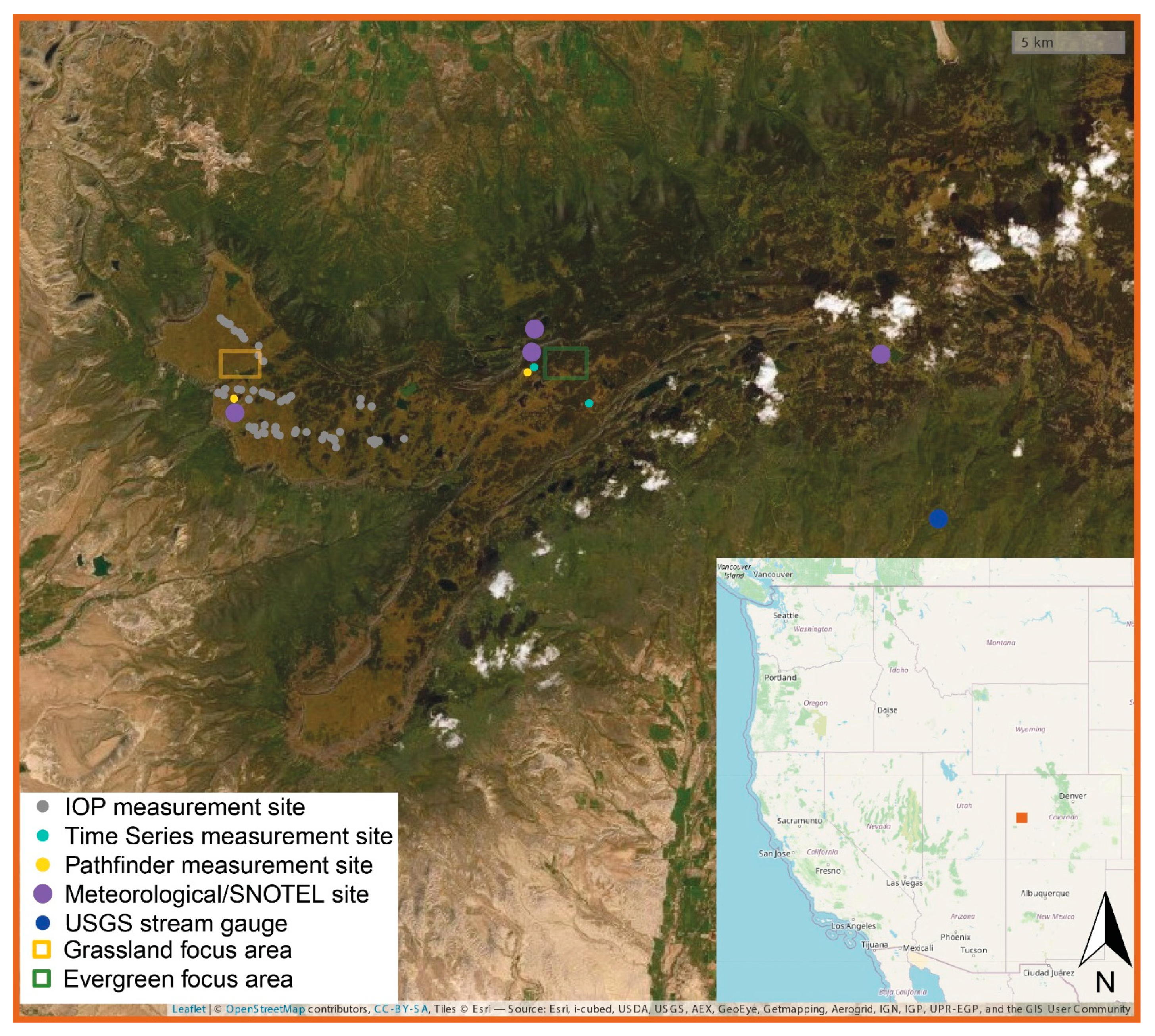
2.1. Study Area: Grand Mesa, Colorado, USA

Grand Mesa (Figure 1) is the largest flat top mountain in the world, encompassing about 1300 km² above 3000 m; the average elevation is 3145 m. Dominant land covers on the Mesa are grassland/herbaceous and evergreen trees. The Mesa Lakes SNOTEL site, located on the north–central part of the Mesa, calculates a 30-year median (1991–2020) of 84.8 cm annual precipitation, 45.5 cm (w.e.) of which falls as snow. Median snow onset takes place on October 23; the median melt-out date at this location is June 1. The median annual average temperature is 1.8 °C.

Grand Mesa was a focal point of the field study for the NASA SnowEx campaign, with an intensive multi-week field campaign in January/February 2020 where physical snow measurements as well as a multitude of ground-based and airborne instruments capturing snow properties were deployed. It was also one of the SnowEx 2020 Time Series sites, with weekly measurements from December 2019 to March 2020. With regard to this study, the consistent topography of the Mesa top offers an opportune venue to study snowpack processes prior to melt-out, as the spatiotemporal variability inherent in these processes is not compounded by topographic complexity.

2.2. Data

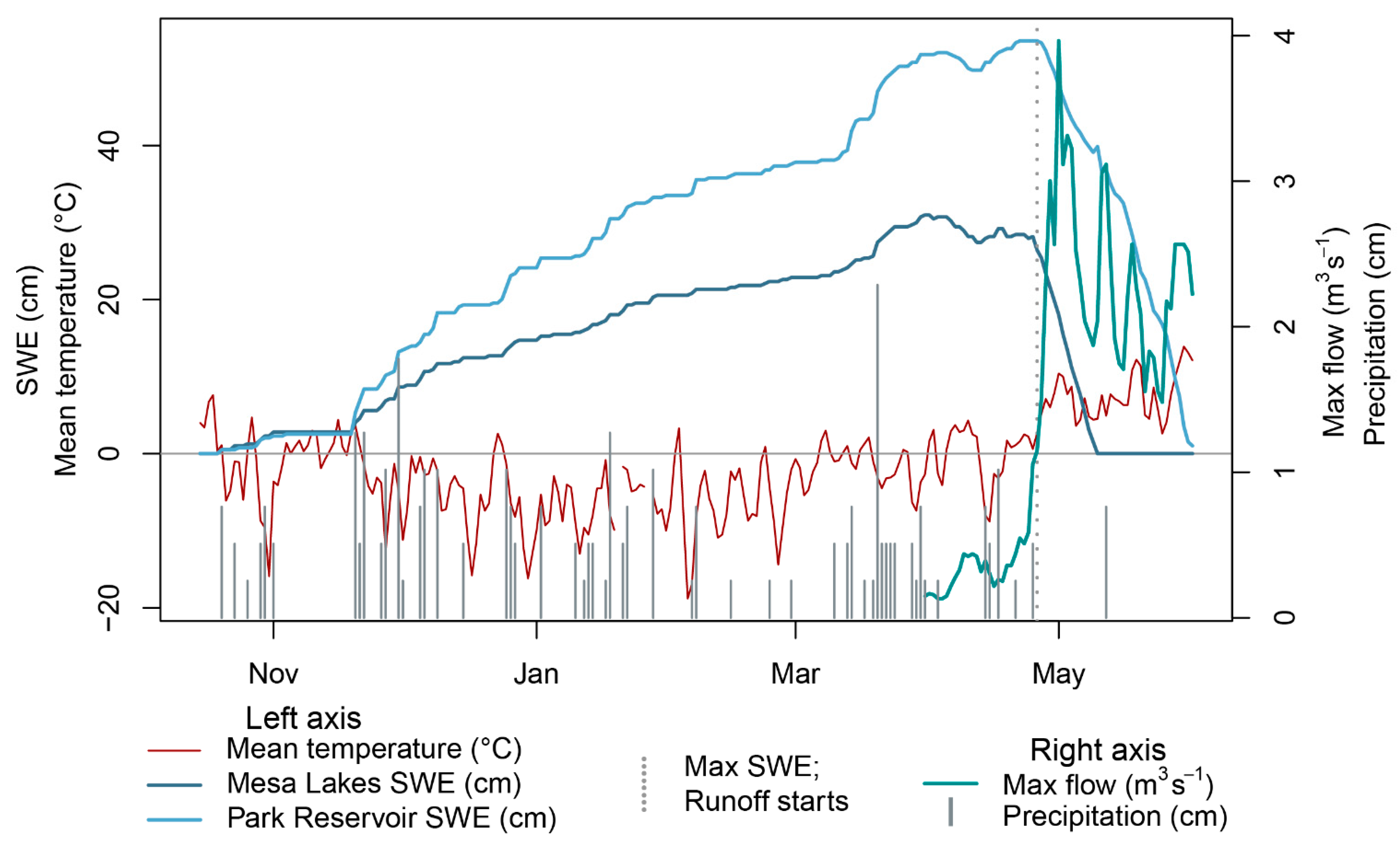
2.2.1. Meteorological and Streamflow Data

Major meteorological variables were gathered from four primary sites (Figure 1, purple): (1) the Mesa Lakes Natural Resource Conservation Service (NRCS) SNOTEL site [52], (2) the Park Reservoir NRCS SNOTEL site, (3) the nearby Skyway Snow Study Plot, downloaded from MesoWest and made available through the Colorado Avalanche Information Center and the Meteorological Assimilation Data Ingest System) [53], and (4) the NASA SnowEx Mesa West study plot. Site locations are listed in

Table 1. Meteorological and streamflow sites used.

Site	Latitude, Longitude	Elevation (m)	Organization
Mesa Lakes SNOTEL	39.06, −108.06	3099	NRCS
Mesa West Study Plot	39.03, −108.21	3033	SnowEx
Park Reservoir SNOTEL	39.05, −107.88	3044	NRCS
Skyway Study Plot	39.05, −108.06	3239	CAIC
Surface Creek Stream Gauge	38.98, −107.85	2521	USGS

. Meteorological variables (air temperature, relative humidity, wind speed and direction, and precipitation) on a 3-hourly time step were used as inputs for SnowModel. A few SWE measurements from the Mesa Lakes SNOTEL site were also incorporated into SnowModel. Select environmental variables from the Mesa Lakes and Park Reservoir SNOTEL sites, as well streamflow measurements from the US Geological Survey (USGS) Surface Creek stream gauge ([54]; Figure 1, blue), are presented in the Section 3 to provide context for the snow accumulation and ablation seasons.

2.2.2. Snow Pit Measurements

Snow pit measurements were gathered from three related field campaigns: (1) the SnowEx Time Series campaign of winter 2019–2020 (hereafter referred to as Time Series) gathered snow measurements from 13 different locations throughout the western United States weekly from December 2019 through March of 2020 (Figure 1, cyan). These measurements were ended early in March 2020 due to the onset of the COVID-19 pandemic; (2) the SnowEx Intensive Observation Period on Grand Mesa (hereafter referred to as IOP) from 28 January –12 February 2020 dug and measured 154 snow pits [55] (Figure 1, grey); and (3) research supported by the CUAHSI Pathfinder Fellowship (hereafter referred to as Pathfinder), which took place in March and April 2020; 51 pits were dug at two primary site locations on the Mesa, matching measurement protocols with the SnowEx Time Series and IOP campaigns (Figure 1, yellow). Pit measurement data, including date, location, and associated campaign, are listed in Table S1. All of the pit measurements referenced in this study, from all three related campaigns (Pathfinder measurements were consolidated with Time Series measurements), are or will be available through the National Snow and Ice Data Center (NSIDC) [56].

Snow pit variables used include snowpack temperature, permittivity, density, and stratigraphy; measurement protocols and instrumentation are described in [55]. The temperature was measured at the snow surface and 10 cm intervals with depth with a Copper-Atkins digital thermometer, with a resolution of 0.1 °C and accuracy of ±1 °C. Snow permittivity was measured using an A2 Photonics WISe instrument, measured every 10 cm with depth. This is utilized with density measurements, also taken every 10 cm with depth, using a 1000 cc wedge-shaped Snow Density sampler and with an accuracy of ±1% by volume along with an AD-3000 digital scale with 1 g resolution and 1 g repeatability. Stratigraphy was also measured for the snowpack; manual wetness for each layer, rated on a five-point scale (dry, moist, wet, very wet, soaked), was used in this study. Manual wetness is determined by varying levels of snow cohesion as well as perceived moisture.

While the SnowEx Time Series and IOP snow pit times and locations were determined in line with SnowEx 2020 overarching objectives, the Pathfinder snow pits were dug on coincident dates, and as near in time as possible, to S1 overpasses. Pits were dug and measurements made in between S1 overpasses as well, to track snowpack conditions with depth throughout snowpack warming and ripening. Pit measurements were used to provide information about snow conditions at the time of (and in between) S1 overpasses, and measured SWE was also used to inform SnowModel runs.

2.2.3. European Space Agency Sentinel-1 SAR Imagery

Operating at a center frequency of 5.407 GHz (C-band, 5.5 cm), the ESA S1 constellation was first launched in April 2014 with Sentinel-1A. After the launch of Sentinel-1B in April 2016, revisit times for much of the western United States are 12 days for each ascending and descending pass in dual polarization (VH and VV). Local acquisition times are approximately 7:18 and 19:10 Mountain Daylight Time for descending and ascending passes, respectively. Ground range detected high-resolution imagery from July 2019 through June 2020 were downloaded from the Alaska Satellite Facility Distributed Active Archive Center [57] and processed using the open-source ESA Sentinel Application Platform (SNAP) [58], adapted from [38]; Figure 2). Images used in the analyses are listed in Table S2; the entire study area is within one S1 frame for both ascending and descending orbital passes.

2.2.4. Copernicus Digital Elevation Model

The ESA Copernicus GLO-30 digital elevation model (DEM), at a resolution of 30 m, was used for S1 processing and analysis; these data are freely available through ESA SNAP software as well as through the ESA’s Copernicus Space Component Data Access portal [59].

2.2.5. Landcover

The National Landcover Database (NLCD) 2019, a 30 m Landsat-derived landcover dataset available from the USGS, was used to identify dominant landcover classes on the Mesa top to focus backscatter analysis [60].

2.3. Methods

2.3.1. Snow Pit Measurement Comparison and Integration

From the snow pit measurements collected from the Time Series, IOP, and Pathfinder campaigns, we implemented a decision tree method to compare measured snow conditions to S1 diurnal snow conditions. For a given date, we gathered all pits measured in open spaces (i.e., without tree cover). Upon cursory comparison for snow pit measurements at depth for each date, we found that snow conditions in treeless areas were very comparable at different locations on the Mesa (e.g., when bulk snowpack temperatures were either subfreezing in the winter or warming in spring, these general temperature ranges were consistent at different study sites). With this consistency in mind, we present the nearest in-time pit measurements to S1 overpass times (approximately 7:00 and 19:00 Mountain Daylight Time). We utilized pit measurements of temperature at depth (taken at 10 cm intervals), as well as manual wetness measurements (taken at depths determined by snowpack stratigraphy). For standardized comparison and visualization with depth, we interpolated stratigraphic manual wetness measurements to even 10 cm intervals. We also utilized measured permittivity and snow density to compare a range of LWC values with manual snow wetness measurements. Presented pit measurements offer insights, discrete in space and time, into snowpack conditions during winter, warming, ripening, and runoff phases, which we used to interpret S1 diurnal snow conditions during those same timeframes.

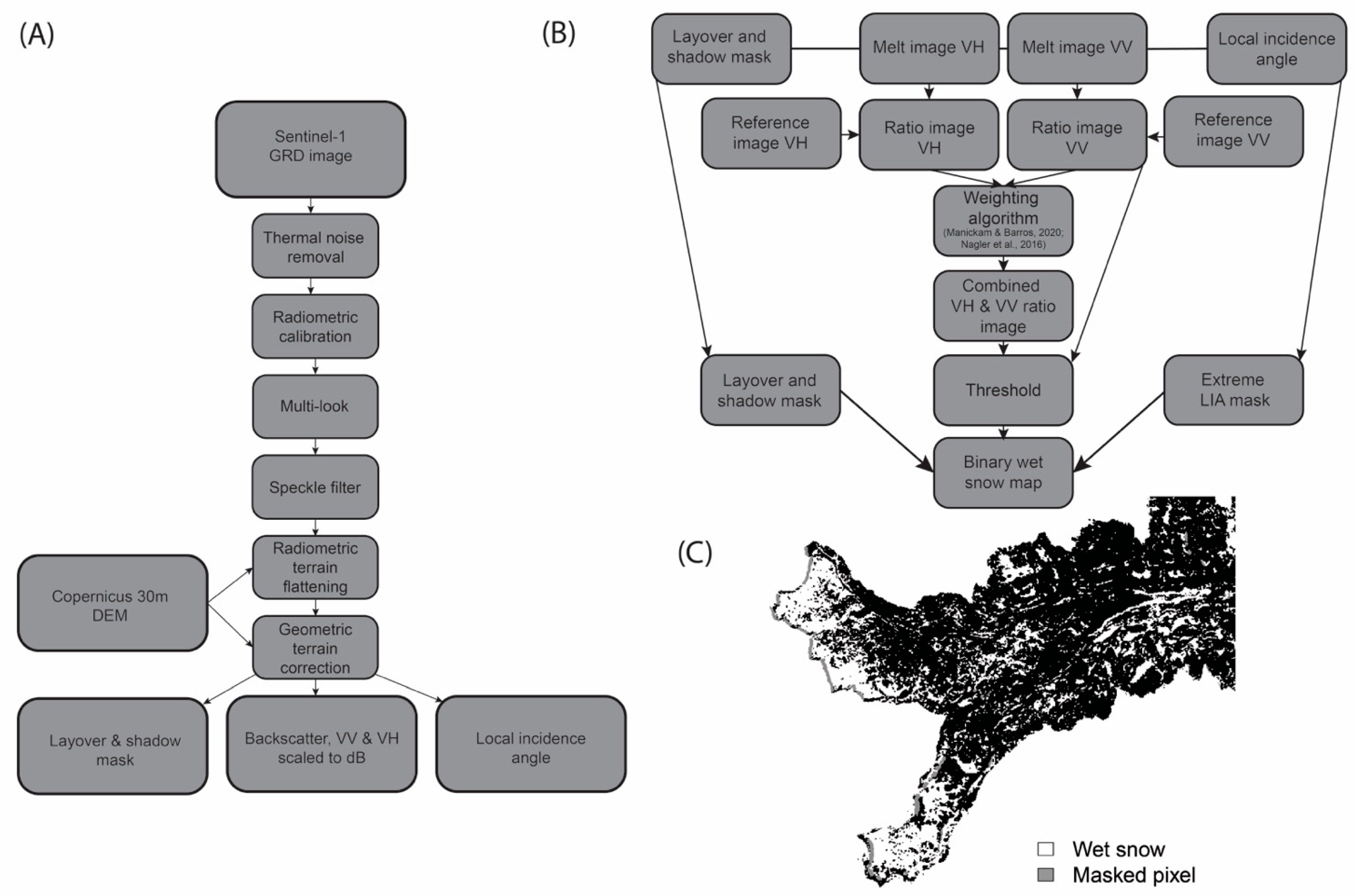
2.3.2. Sentinel-1 Diurnal Wet Snow

S1 image processing workflows can be viewed in Figure 2A, adapted from [38] using ESA open-source SNAP software [58]. The output of SAR processing is radiometric terrain corrected [61] gamma nought (γ₀) backscatter image for a given date, at 30 m resolution. Backscatter values for two dominant land cover classes on the Mesa, grassland/herbaceous and evergreen forest, are explored from 2019–2020.

Figure 2. (A) Sentinel-1 processing steps, performed in the European Space Agency’s SNAP open-source software; (B) Backscatter image threshold wet snow identification process, accomplished in R [62]; (C) Example binary wet snow map.

Figure 2. (A) Sentinel-1 processing steps, performed in the European Space Agency’s SNAP open-source software; (B) Backscatter image threshold wet snow identification process, accomplished in R [62]; (C) Example binary wet snow map.

For wet snow identification, multiple threshold-based change detection algorithms were explored for the Mesa. Processed melt season images were first co-registered with a reference image, which was an average of several co-registered images from antecedent snow-free (July–August 2019) and/or dry snow (December 2019–January 2020) conditions, and the ratio of the two images was calculated (Figure 2B). This ratio image was developed for three different peer-reviewed wet snow threshold approaches: (1) −2 to −3 dB threshold using either co- (VV) or cross-polarized (VH) ratios [21,27,28,29,30,31]; (2) −2 dB threshold using both co- and cross-polarized ratios, combined by weighting ratio values according to local incidence angle, following the algorithm developed by [34]; and (3) −1.2 dB threshold using both co- and cross-polarized ratio images, combined by weighting ratio values according to cross-polarized image ratio thresholds, following the algorithm developed by [33] specifically for wet snow identification on Grand Mesa. For all three threshold algorithms, pixels with a ratio value at or below the specified threshold were designated as ‘wet snow;’ to reduce the impact of noise, a 3 × 3 moving window was then applied to determine binary wet/not wet snow (Figure 2C, white). Pixels with local incidence angles less than 15 or greater than 75 degrees, as well as pixels affected by layover or shadow, were masked out (less than 1% of the analyzed area) [34]. Water bodies, identified through the NLCD 2019 dataset [60], were also masked (Figure 2C, gray).

To generate a diurnal S1 snow conditions map, we first selected only snow-covered pixels (determined from SnowModel outputs) above 2900 m to limit the study to the Mesa top. Next, with binary wet snow maps generated for each orbit, coinciding descending (morning) and ascending (evening) passes were compared pixel-wise using the method generated in [38], with four possible output categories: (1) pixels that register as wet for both morning and evening passes, (2) pixels assigned not wet in the morning but wet in the evening; (3) pixels determined wet in the morning but not in the evening; and (4) pixels that do not register as wet in either pass (labeled SnowModel snow). An example of morning and evening wet snow identification, resulting in a diurnal S1 snow conditions map, is shown in Figure 3. All post-processing steps and analyses were accomplished in R [62].

2.3.3. SnowModel

In order to capture the diurnal cycle, we run SnowModel from [39] on a three-hour time step, with meteorological and environmental inputs specified in Section 2.2.1. We incorporate measured bulk SWE from 69 snow pit measurements (Supplementary Table S1) from Time Series, IOP, and Pathfinder campaigns as described in Section 2.2.2. We also incorporate three SWE measurements from the Mesa Lakes SNOTEL site, to refine snow onset and melt-out dates at that location. We track variables such as SWE, snow melt, and runoff, along with energy balance variables such as air temperature and net radiation, for one of the selected snow pit measurement locations throughout snow accumulation and ablation seasons.

We also utilize spatially distributed SnowModel outputs of SWE, snow surface melt, and snowmelt runoff to compare with surface states derived from S1 diurnal snow conditions. SnowModel surface melt below a threshold of 0.35 cm is ignored, to facilitate S1 diurnal comparison, which we find insensitive to minor surface melt. If snow runoff is calculated for three timesteps the day before and the day of diurnal comparison, SnowModel diurnal comparison determines that pixel to be in the ‘runoff’ phase, comparable to S1 diurnal outputs that show snow as wet in both morning and evening overpasses. The model, driven by local meteorological data and refined by the assimilated SWE measurements, presents a continuous representation in space and time of snowpack conditions, extending information beyond discrete field measurements. This assimilation of the model increases confidence in S1 diurnal snow conditions interpretation.

3. Results

3.1. Field Measurements

To provide the seasonal context for our pit measurements and remote sensing results, we first present relevant environmental variables from nearby SNOTEL sites and streamflow from the nearby USGS Surface Creek gauge. We next share a narrative of researcher-experienced meteorological and snowpack conditions during the snow season, along with snow temperature and wetness measured in the field. After providing results of Sentinel-1 diurnal snow conditions and SnowModel outputs, we offer an integrated and complementary perspective of snowpack conditions and associated S1 diurnal interpretations.

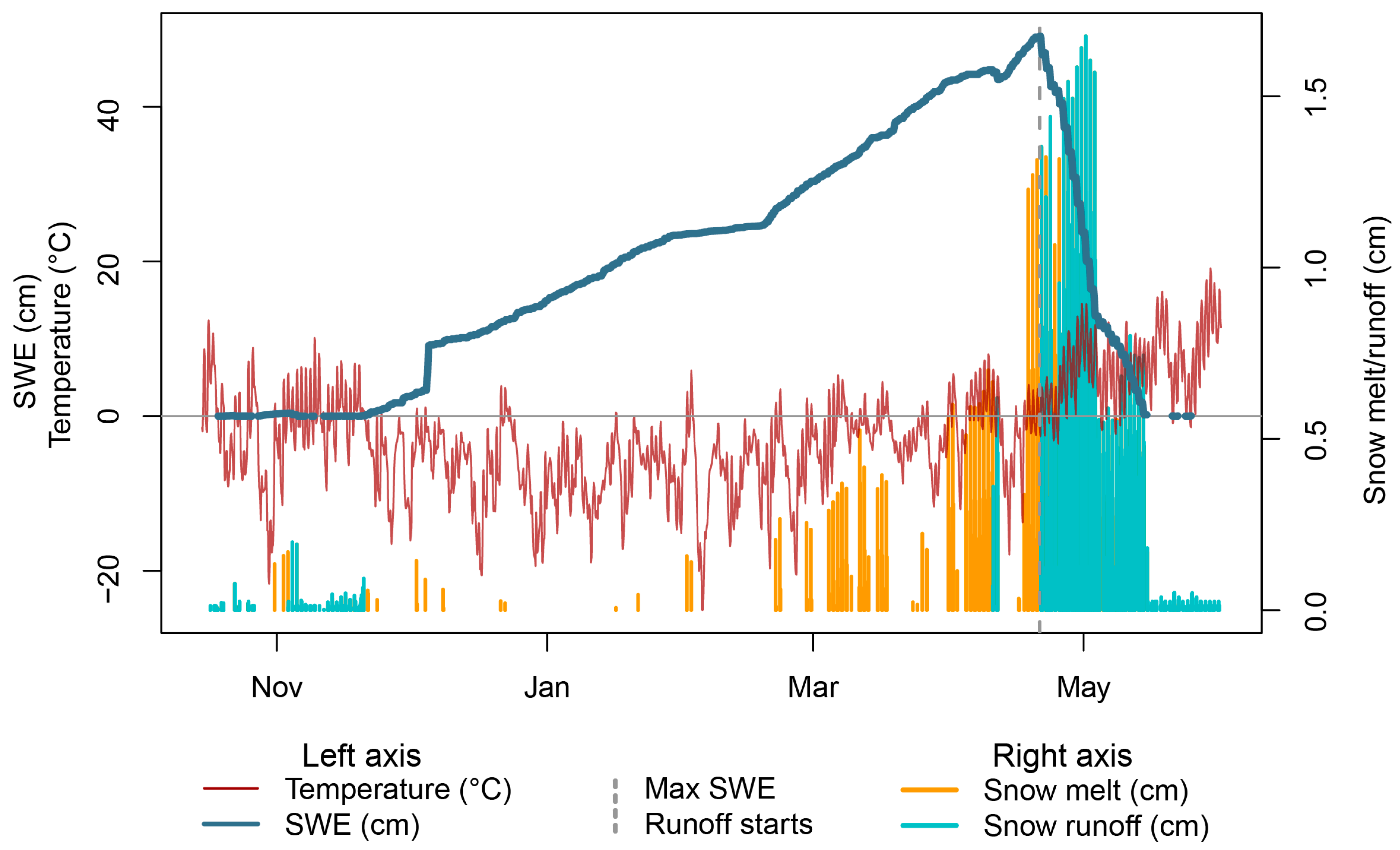
3.1.1. Environmental Variables

In order to specify snow accumulation and ablation seasons, select environmental variables from the Mesa Lakes and Park Reservoir SNOTEL sites and streamflow from the nearby USGS Surface Creek gauge are shown in Figure 4. Mean daily temperatures (Figure 4, red) were mostly below freezing in December through February. In March, mean temperatures oscillated above and below freezing. A significant snow storm arrived in the third week of March (Figure 4, grey), which coincided with a reduction in temperatures. Both SNOTEL sites show a local SWE maximum in early April (31 cm at Mesa Lakes, 52 cm w.e. at Park Reservoir), and runoff (Figure 4, cyan) began shortly thereafter, coinciding with mean temperatures above freezing. However, runoff stalled as a snowstorm and a decrease in temperatures occurred in mid-April. Maximum SWE at the Park Reservoir SNOTEL calculates about 54 cm w.e. on 22–26 April. In late April and early May, temperatures remained significantly above freezing. This coincided with an uninterrupted reduction in SWE and a corresponding increase in runoff. Sustained seasonal runoff (above 1 m³·s⁻¹) is identified at the USGS Surface Creek stream gauge starting on 24 April (dotted line). Snow melt-out takes place on May 10 at Mesa Lakes and 3 June 2020, at Park Reservoir SNOTEL sites.

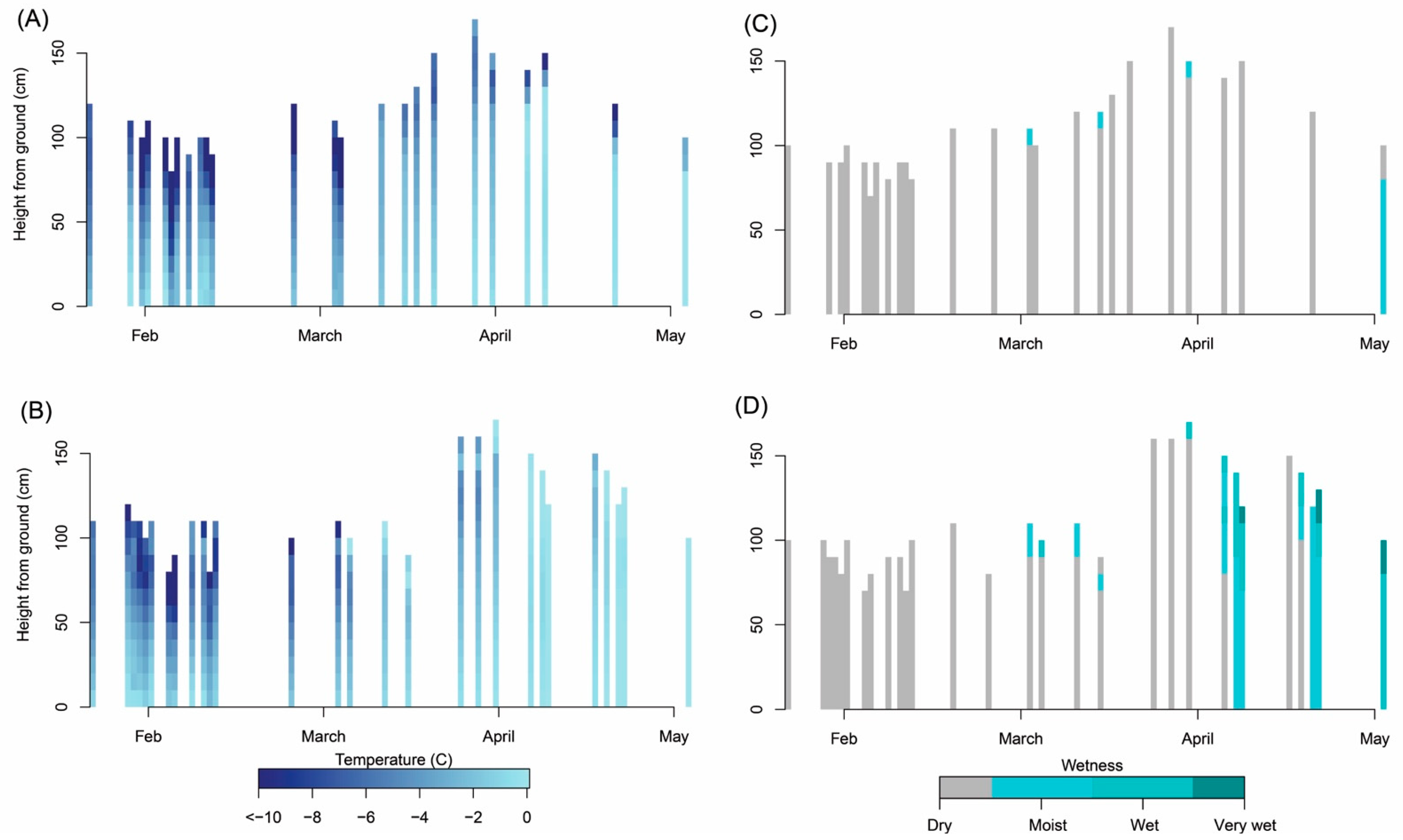
3.1.2. Snow Pit Measurements

Figure 5 shows measurements of snowpack temperature (Figure 5A,B) and wetness (Figure 5C,D), with depth and over time. For comparison, morning and afternoon measurements are separated on the top and bottom rows, respectively.

The snowpack remained dry, with sub-freezing temperatures at the surface and with depth, throughout the winter season (December through February) until early March, when above-freezing temperatures and sunny conditions coincided with the first signs of surface melt and snowpack warming. For the first two weeks of March, surface moisture was noted by researchers in both morning and afternoon snow pits in the topmost stratigraphic layers of the snowpack; however, only afternoon measurements showed snow surface temperatures near 0 °C. In the third week of March, air temperatures dropped and snow fell; surface melt ceased. Beginning in early April, air temperatures increased and significant melt-freeze cycles took place over a rapidly warming and ripening snowpack. On 9 April, significant melt/freeze crusts, ice pipes, and ice lenses on the order of several centimeters within the top 40 cm of the snowpack in morning measurements were noted; evening measurements recorded the snow as wet or moist throughout the depth of the snowpack, though some layers were still subfreezing. In mid-April, incoming snow added significant cold content to the snowpack and coincided with a decrease in air and snowpack temperatures. Melt resumed in the third week of April, and the snowpack rapidly warmed and ripened again. Researchers noted wetness in the snowpack ranging from moist to very wet on the afternoons of 21 and 22 April, though some layers still measured subfreezing temperatures. In early May, melt-out was well underway; a 15 cm melt/freeze crust, which required a snow saw to excavate, had developed over a wet and isothermal snowpack on the morning of 3 May; this crust rapidly warmed and melted that afternoon. Researchers were not present for snowpack melt-out.

With these field measurements in mind, we identify the snowpack warming phase primarily taking place in March, when the bulk snowpack temperatures increased relative to January and February temperatures and surface melt, typically in the top 10 cm of the snowpack, was initiated. We identify snowpack ripening developing rapidly in April, where bulk snow temperatures were at or very near 0 °C and the snow was noted as dry throughout the depth of the snowpack in morning pits, and wetness ranged from moist to very wet throughout the depth of the snowpack in afternoon measurements. A ripe snowpack contributing to runoff is identified in May measurements, with morning measurements showing bulk temperatures at −0.2 °C (beneath a sub-freezing refrozen surface crust) and wetness measurements ranging from wet to very wet in both morning and afternoon pit measurements. It may be noted that these identified phases are generalizations of complex and variable processes at the boundary of and within the snowpack; in both mid-March as well as mid-April, snowstorms added significant cold content to the snowpack and cloudy skies and reduced air temperatures impacted the snow surface energy budget.

3.2. SnowModel

To explore simulated snow conditions, we first present SnowModel output variables at a primary Pathfinder measurement site location on the northwestern lobe of Grand Mesa (Figure 1, yellow), to compare with SNOTEL environmental variables in Figure 4 and field-measurement indications of the snowpack phase in Figure 5.

Figure 6 shows relevant SnowModel variables at the Mesa West Pathfinder measurement site throughout the 2020 snow season. At this site, SWE (Figure 6, blue) increased throughout the winter until early April and reached a maximum of 49 cm w.e. on 20 April. A comparison of simulated and observed SWE measurements may be found in Figure S1, which calculated an adjusted R-squared of 0.87. Minimal surface melt was calculated on a few days in February; minor surface melt (less than 0.5 cm) was generated throughout March and more significantly (greater than 0.5 cm) in early April (Figure 6, orange). Beginning 10 April, the snowpack ripened and runoff began, coinciding with a slight decrease in SWE. However, on 12 April runoff ceased as air temperatures decreased and snow fell, adding cold content to the snowpack. In the third week of April, significant surface melt was generated; runoff from the snowpack (Figure 6, cyan) was sustained starting 21 April. Snowpack melt-out at this location occurred on 16 May. Comparing these outputs with field measurements, we conclude that snowpack warming in March took place when surface snowmelt of less than 0.5 cm was simulated. Melt over 0.5 cm, which took place starting in April, we associate with the ripening phase. SnowModel calculated runoff from the snowpack briefly from 10–11 April, and then again starting on 21 April; the snowpack runoff phase is identified beginning on this date.

3.3. Sentinel-1

To provide a framework for algorithms and thresholds used in S1 diurnal comparisons, we first explore S1 co- and cross-polarized backscatter values from July 2019–June 2020 for two focus landcover areas: grassland/herbaceous, and evergreen (focus areas labeled in Figure 1). These analyses, with field measurements and SnowModel indications of snow conditions throughout the season, are used to inform our selected algorithm and threshold, which we then use to present and assess a seasonal diurnal S1 snow conditions time series.

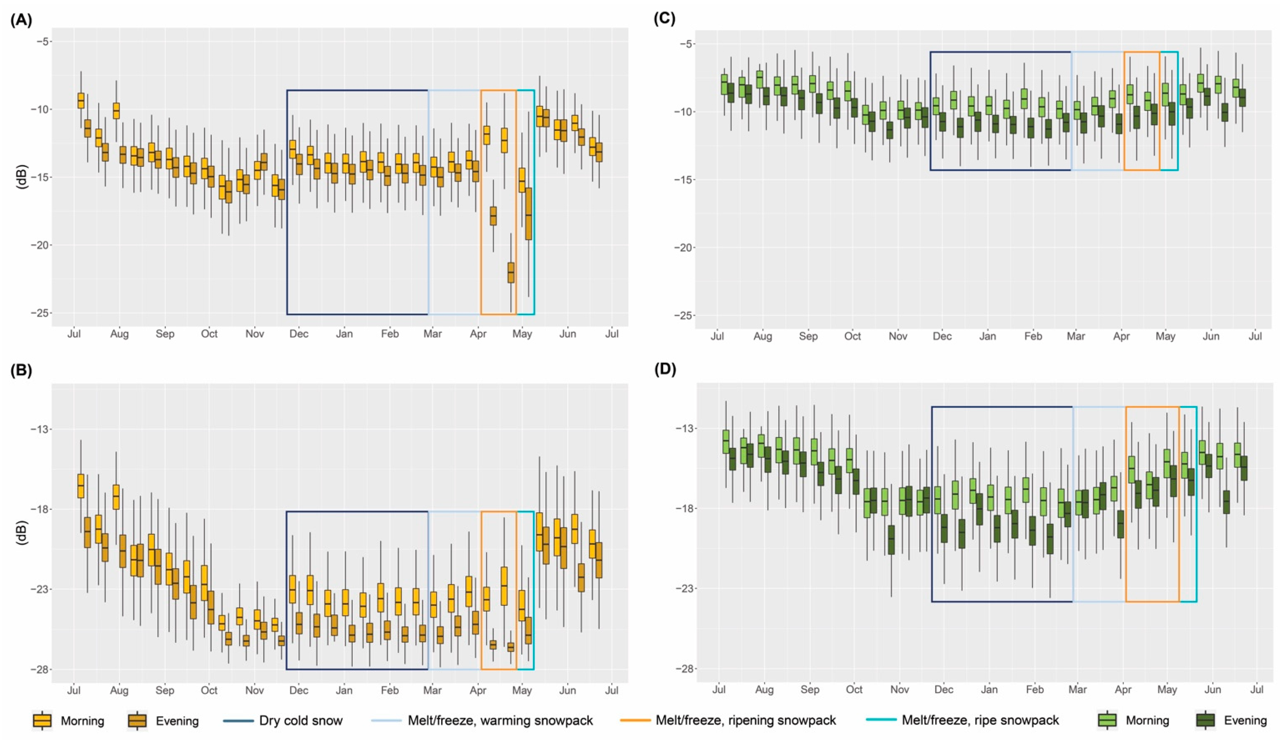
3.3.1. Land Cover Backscatter Values

Figure 7 shows backscatter values over time for two dominant landcover classes on Grand Mesa: grassland (Figure 7A,B, 1843 pixels) and evergreen (Figure 7C,D, 2005 pixels). These are differentiated according to co- and cross-polarizations (top and bottom rows, respectively) for each landcover. We highlight time periods where field measurements and SnowModel outputs indicated a dry winter snowpack (Figure 7, dark blue box), surface melt/freeze cycles over a warming snowpack (Figure 7, light blue box), surface melt/freeze cycles over a ripening snowpack (Figure 7, orange box), and surface melt/freeze over a ripe snowpack contributing to runoff (Figure 6, cyan box), as discussed in Section 3.1.2 and Section 3.2. For grassland cover, both co- and cross-polarizations showed consistent values for morning and evening overpasses in the months of December through February (Figure 7A,B, dark blue box). During snowpack warming and initial surface melt/freeze in March, neither orbital pass nor polarization showed a noticeable change in backscatter (Figure 7A,B, light blue box). Grassland co-polarized (VV) backscatter values in the morning measured a significant increase during surface melt/freeze cycles over a ripening snowpack, a median of 1.8 (±1.2) dB and 1.5 (±1.5) dB on 9 April and 21 April, respectively (Figure 7A, orange box). Morning VV backscatter values decreased for surface melt/freeze over a ripe snowpack (3 May acquisition) by −1.5 (±1.3) dB (Figure 7A, cyan box). Evening VV backscatter values showed significant decreases throughout the ripening and runoff phases of the snowpack, the most significant of which calculated a median of −7.5 (±1.3) dB on the evening of 21 April, a median diurnal difference of −9 dB (Figure 7A, orange box).

Morning VH backscatter values did not show a noticeable difference during snowpack warming, ripening, or runoff phases (Figure 7B, light blue, orange, and cyan boxes, respectively). Evening VH backscatter values decreased slightly (−0.2 to −1.2 dB) during the afternoon melt for the snowpack ripening and runoff phases.

Snowpack melt-out in mid-May coincided with an increase in backscatter values for both co- and cross-polarized values for both morning and evening overpasses. As backscatter values were most consistent in dry snow conditions (December and January), images from this timeframe were subsequently selected to create the reference image used for threshold algorithms.

Evergreen backscatter values did not show distinct changes during snowpack surface melt/freeze cycles, warming, or ripening (Figure 7C,D). Evening VH backscatter values were variable throughout the snow accumulation and ablation seasons. Because of the indistinct backscatter responses to different snowpack conditions, as well as the potential for inter-image backscatter variability (with tree branches and needle sizes on the order of C-band wavelength, 5–6 cm), and also a significant difference in boundary energy fluxes for canopy snow compared to snow on the ground, we constrained S1 and snow pit analyses solely to areas without tree cover.

From these analyses, which show less sensitivity of cross-polarized backscatter to surface melt and refreeze compared to co-polarized backscatter, along with results from testing the threshold algorithm outputs for multiple threshold algorithms listed in Section 2.3.2 (see Appendix A and Appendix B), we selected a co-polarized −2 dB threshold algorithm to explore S1 diurnal snow conditions throughout the snow season of 2020.

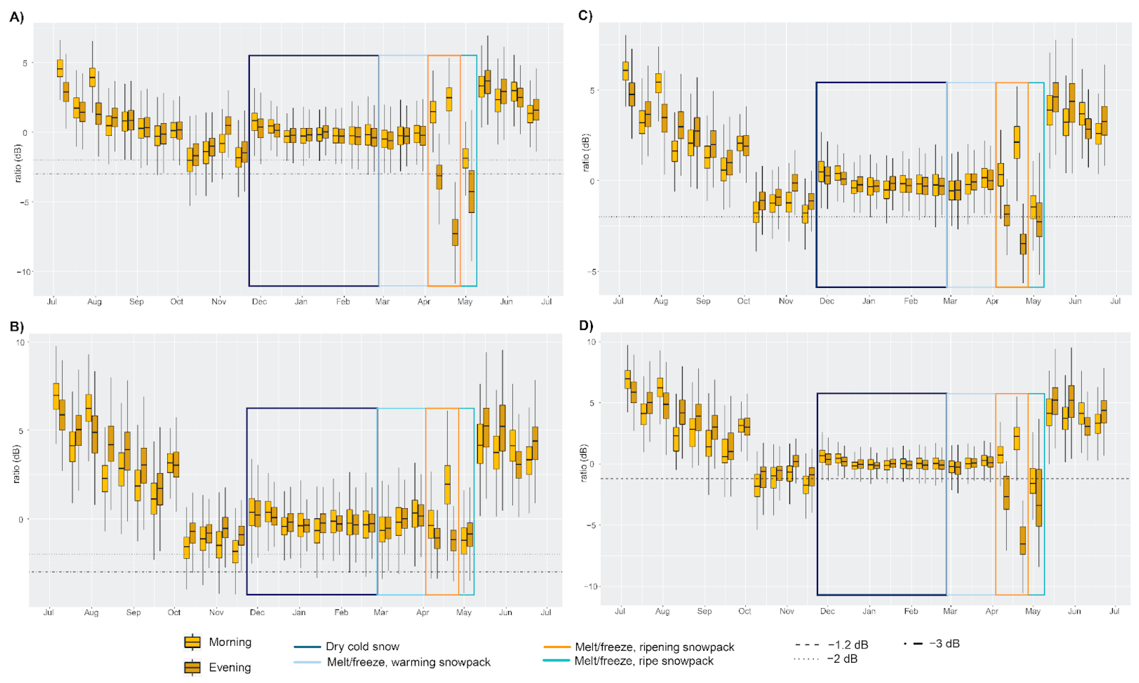
3.3.2. Sentinel-1 Diurnal Wet Snow

Figure 8 shows the S1 diurnal snow conditions time series from 28 January to 3 May 2020. Images from overpass dates with coincident field measurements indicate pit locations.

S1 diurnal snow conditions remained dry throughout the winter until 16 March, when some pixels on the southern and south facing, lower elevation edge of the Mesa showed signals of melt/freeze (Figure 8E, southwest lobe). In April, surface melt/freeze cycles were prevalent on the western lobes of the Mesa, with pixels classified as dry in the morning and wet in the evening S1 overpasses (Figure 8G,H). On 3 May, many pixels were classified as wet in both morning and evening overpasses, though some pixels on the northwest lobe of the Mesa were classified as dry in the morning and wet in the evening (Figure 8I). From backscatter analyses and diurnal snow condition outputs, we infer that S1 diurnal wet snow methods were insensitive to the initial snowpack warming phase in March. In April, during snowpack ripening with significant surface melt/freeze, Figure 8G,H shows a diurnal difference in S1 SAR snow conditions (orange). During the runoff phase, many pixels were determined ‘wet’ in both morning and evening overpasses (Figure 8I, cyan).

3.4. Integration

In the following sections, we provide an integration of field measurements and SnowModel simulated snow conditions, which we utilize to interpret S1 diurnal backscatter response and derived snow conditions.

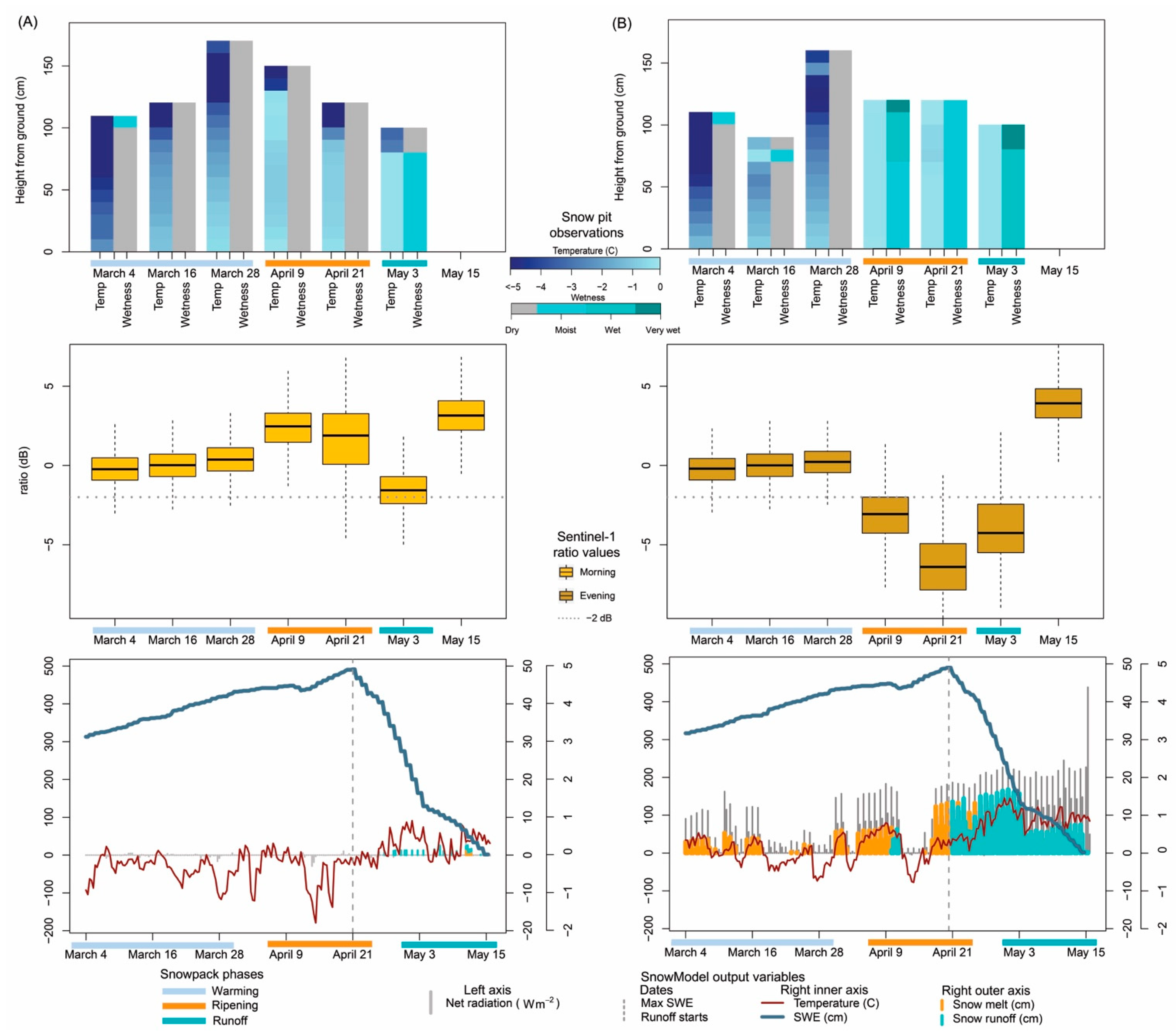
3.4.1. Snowpack Phases and S1 Backscatter

Figure 9 compares field measurements of temperature and wetness (Figure 9, top row) with S1 ratio values (Figure 9, middle row for easy comparison) as well as SnowModel output variables, such as SWE, air temperature, net radiation, and snowpack melt and runoff (Figure 9, bottom row). Comparisons are made from 4 March to 15 May 2020. These are separated by morning and afternoon timeframes (Figure 9A,B, respectively). Snowpack phases of warming, ripening, and runoff, determined from field measurement and SnowModel outputs, are highlighted on the x-axes (Figure 9 light blue, orange, and cyan, respectively). Though field measurements were taken in between S1 overpass dates, only coincident measurements are shown for clarity.

Figure 9 highlights significant differences in both field-measured and SnowModel estimated snow conditions (and associated net radiation), in between morning and afternoon timeframes as well as through identified snowpack phases of warming, ripening, and runoff. The comparative figure clearly indicates that the S1 backscatter ratio, in both morning and evening overpasses, is not sensitive to snowpack warming and minor surface melt (less than 0.35 cm) in March. During snowpack ripening in April, with significant surface melt/freeze cycles, morning S1 backscatter increased by medians of 1.8 and 1.5 dB, and afternoon backscatter decreased, with median changes of −3.4 and −7.5 dB. During the runoff phase on 3 May, both S1 morning and evening backscatter values decreased, with median changes of −1.5 and −3.0 dB, respectively. S1 diurnal responses in backscatter provide distinct indications of snowpack phase conditions during ripening and runoff phases.

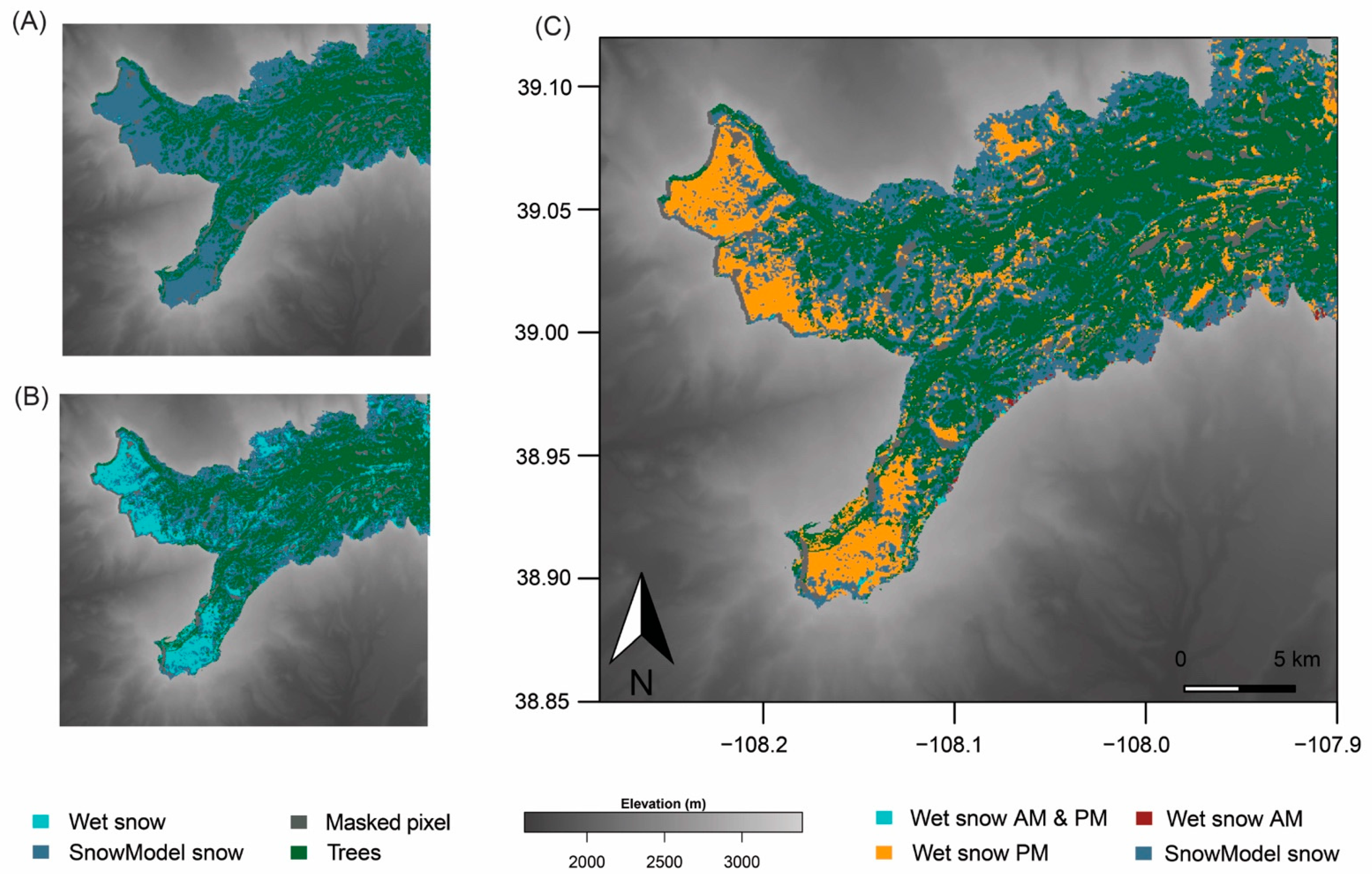
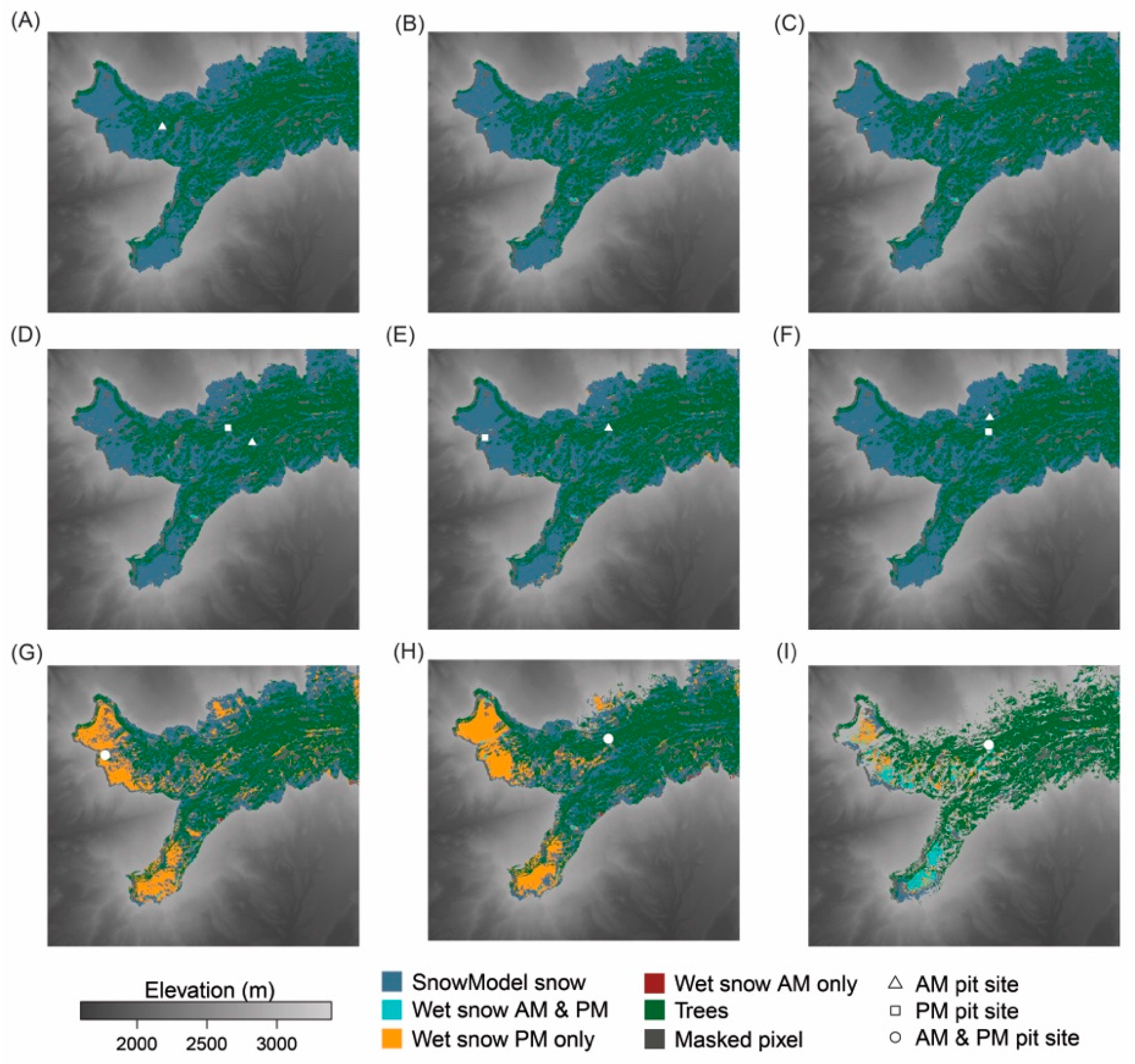
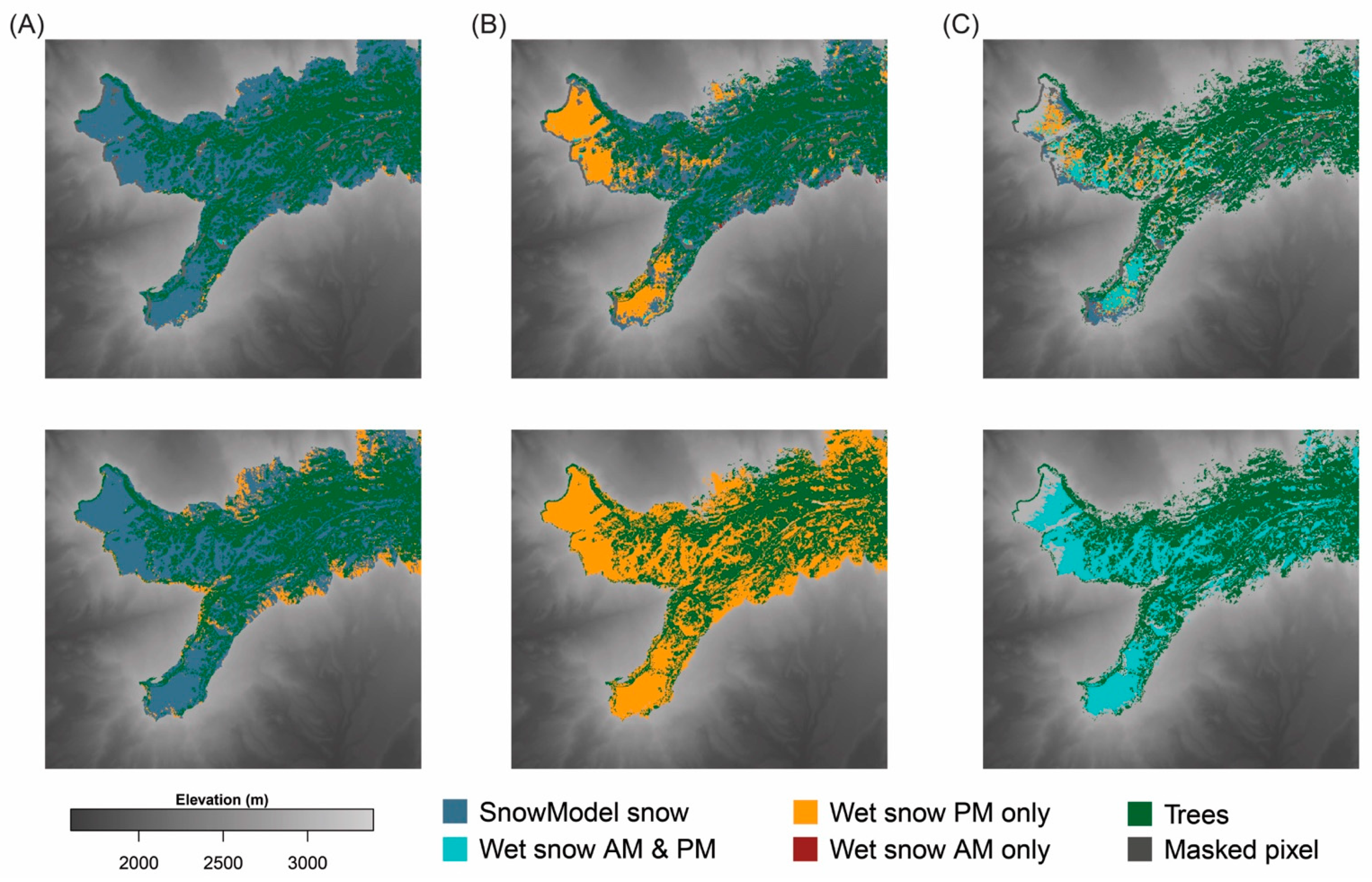
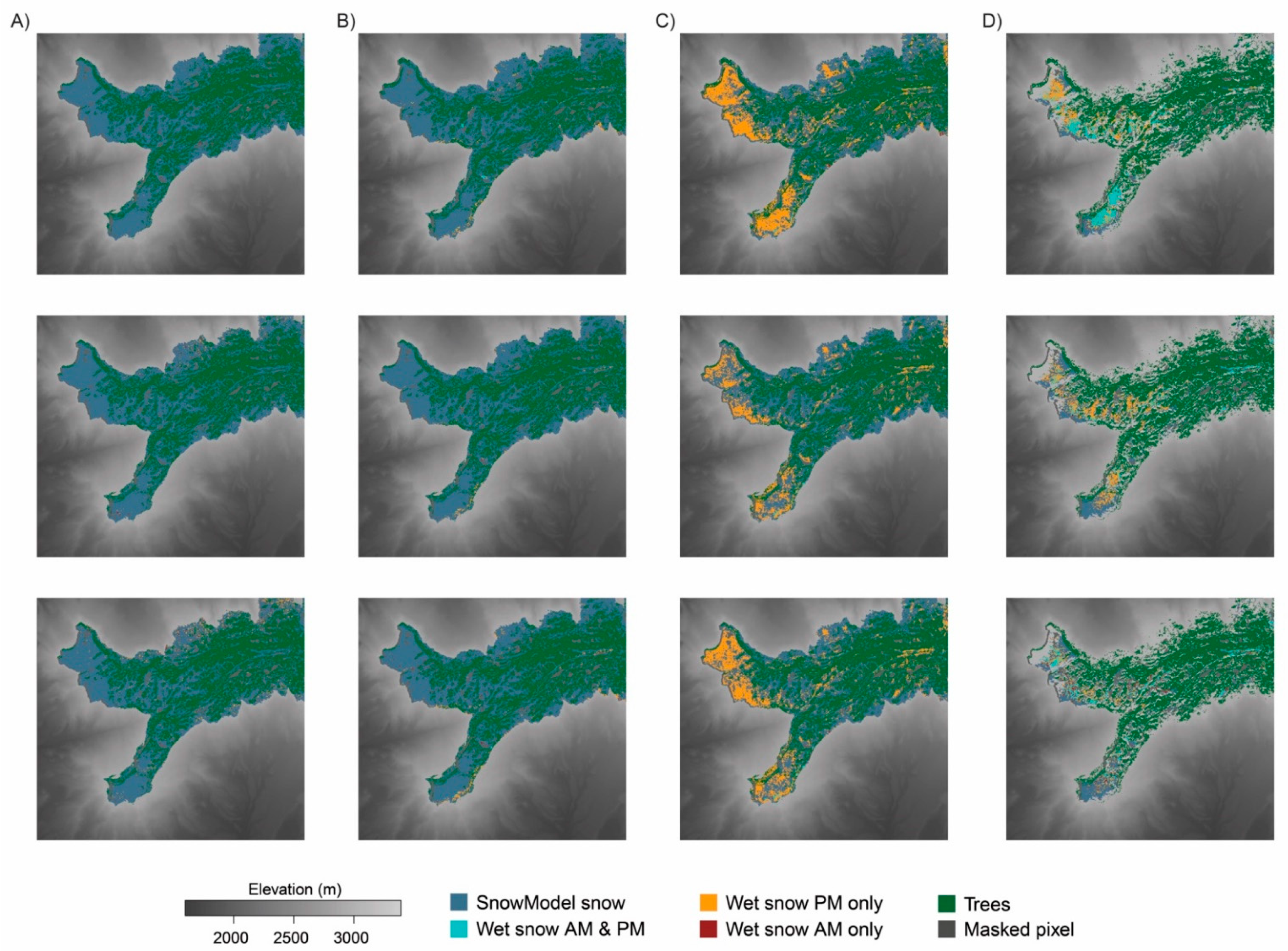
3.4.2. S1 and SnowModel Diurnal Snow Conditions Comparison

Figure 10 compares S1 (Figure 10, top row) and SnowModel (Figure 10, bottom row) diurnal outputs for three dates in the snowpack warming, ripening, and runoff phases: 16 March, 21 April, and 3 May 2020. Images agree relatively well, with dry and cold snow conditions identified on 16 March, while pixels on the northern and southern edge of the Mesa show afternoon melt in SnowModel diurnal outputs, comparable to S1 diurnal pixels identified as wet in the afternoon on the southern edge of the Mesa. The 21 April diurnal comparisons showed snow as dry in the morning and melting in the afternoon for both S1 and SnowModel methods, though more pixels were identified as such with SnowModel. SnowModel diurnal outputs showed the snowpack in the runoff phase on 3 May; S1 diurnal outputs identified many pixels as wet in both morning and evening overpasses, although some were considered dry in the morning and wet in the afternoon.

4. Discussion

4.1. Field Measurements

4.1.1. Environmental Variables

The Mesa Lakes SNOTEL SWE pillow consistently measured less SWE than was measured in the field, while the Park Reservoir SNOTEL site maximum SWE was greater than was measured in the field. Aside from heterogeneity in snow accumulation patterns due to precipitation variability and differing topography and land cover, research has shown inconsistencies between SNOTEL SWE pillow measurements and both accumulated precipitation measurements as well as snow course measurements, especially at higher elevation Rocky Mountain sites (e.g., [63,64]). Both SNOTEL sites showed reductions in SWE in early April, then increasing SWE in mid-April with incoming snow and lower air temperatures; finally reducing consistently beginning the third week of April, 2020. While snowpack warming, ripening, and runoff can be highly variable in space and time, comparing SNOTEL variables with field measurements generally indicated a similar timing for brief runoff initiation in early April, stalling in mid-April, and then becoming isothermal again on 21 April, after which melt-out began in earnest. This timing is corroborated by the USGS Surface Creek streamflow measurement (Figure 4, cyan).

4.1.2. Snow Pit Measurements

Field measurements of snow temperatures, with depth and over time, are in line with what may be expected as a winter snowpack warms and ripens. Surface temperatures point to the interaction of the snow surface with atmospheric energy fluxes, as well as energy exchange within the snowpack. For the afternoon snow pit measurements, occasionally, snow surface temperature had already cooled again, while subsurface temperatures were warmer, indicating the negative energy flux to the atmosphere had not yet cooled these subsurface layers (Figure 5D: 15 March–1 April afternoon temperatures).

Field measurements of snow wetness correlate well with snowpack temperature measurements throughout the snow season, with moisture first noted at the snow surface and wetness increasing over time, first at the surface and then with depth. It may be noted that in early to mid-March, field researchers described morning surface snow layers as moist when air temperatures and snow surface temperatures were below freezing. This may point to the subjective nature of snow wetness measurements and may also point to conditions where the available surface meltwater generated has not yet refrozen. For these dates, SnowModel outputs showed snowmelt was generated in the 9:00–12:00 timeframe, indicating that energy for melt was available in the morning hours.

Assessing snow wetness as snow approaches the melting point is a difficult task, with or without instrumentation. Though A2 WISe-derived LWC values were variable, they ranged from 0 to 0.5% for ‘dry’ snow, 0–2% for ‘moist’ snow, and 0–5% for ‘wet’ snow. ‘Very wet’ snow accumulated at specific horizons in the snowpack that were not in line with permittivity measurement intervals and, thus, did not correlate with the LWC range.

4.2. SnowModel

SnowModel, driven with local meteorological data and refined with SWE measurements, provided continuous indications of snow conditions that were also spatially distributed. We note that, aside from assimilating SWE measurements in SnowModel, other field measurements were not incorporated into the model. With that in mind, the timing for snowpack warming, ripening, and runoff aligns very well with in situ measurements, facilitating greater confidence in S1 SAR diurnal interpretation. While the maximum SWE value in SnowModel compared well with field measurement (48 and 49 cm w.e., respectively), the timing of maximum SWE differed from that of the Mesa Lakes SNOTEL as well as field-measured maximum SWE. Maximum SWE for the nearby Park Reservoir SNOTEL site, further east on the Mesa, takes place on 22–26 April 2020; thus, the SnowModel maximum SWE timing is comparable to those seen elsewhere on the Mesa.

SnowModel also accurately represented the snow surface state throughout the season, and detected afternoon surface melt in the snowpack warming phase, corroborated with field measurements, when S1 SAR did not. As such, SnowModel offers insight into the capacities and limitations of wet snow detection with S1 SAR. As it is physically-based, it also affords exploration into potential driving factors behind snow surface states, as is indicated in Figure 9; surface melt was associated with air temperatures above freezing as well as increased net radiative inputs.

4.3. Sentinel-1

4.3.1. Land Cover Backscatter Values

Surface melt/freeze cycles during snowpack warming in March were not evident in morning or evening S1 backscatter values for grassland/herbaceous landcover (Figure 7A,B, light blue box). As the overpass time is around 7:00 and 19:00, it is likely that melt had not yet been generated in the morning acquisition (as is corroborated by SnowModel outputs), and may have already refrozen by the evening acquisition. It is also possible that not enough surface melt was generated to significantly attenuate the S1 signal for these overpass dates. Afternoon pit measurements for this time period reported melt in the top 2–3 cm of the snowpack; SnowModel calculated up to about 0.35 cm snow melt. Due to constraints with travel and daylight, especially early in the melt season with fewer daylight hours, pit measurements were always taken after morning and before evening S1 overpasses; for this reason, the presence (or lack) of meltwater at the snow surface in these early March evening overpasses was not confirmed with field measurement.

Significant surface melt/freeze cycles that took place during snowpack ripening in April were associated with a significant increase in VV backscatter values, with median increases of 1.8 and 1.5 dB (Figure 7A, orange box). As was mentioned in Section 1.3.1, refrozen crusts cause an increase in backscatter due to the high volumetric scattering and reflection of large refrozen grains, pipes, and lenses [30,34,35,36,37]; our results corroborate this conclusion. To our knowledge, thresholds have not been identified or indicated for positive morning backscatter ratios. From our focused study, we conclude that a +1 dB threshold for morning ratios may not only confirm that the snowpack is not wet in the morning, but also that significant surface melt/freeze is taking place over a not-yet-ripe snowpack, leading to high volumetric scattering which contributes significantly to the backscatter value.

We hypothesize that the co-polarized backscatter ratio value of −1.5 dB for the morning S1 overpass of 3 May, field conditions which indicated a consolidated and relatively homogeneous melt/freeze crust ~15 cm thick over a wet snowpack, was impacted by both the surface melt/freeze crust as well as the moisture of the snow underneath (Figure 7A, cyan box). The ratio value on 3 May for many pixels on the Mesa was near the −2 dB threshold for identifying wet snow (and as such, many pixels in the study area were identified as wet in the morning and evening overpasses). It also calculated a mean decrease of about −3.0 dB from the preceding S1 overpass on 21 April, indicating a significant change in scattering characteristics between acquisitions. From these observations, we postulate that it may be possible to identify surface melt/freeze crusts over an otherwise ripe snowpack by imposing a different ratio threshold for morning overpasses. Because snow melt-out occurred before snow surface conditions were wet in both morning and evening overpasses, this potential morning threshold requires further testing for conclusions to be drawn.

Evening co-polarized backscatter values showed a significant decrease in April and early May, the most significant of which took place on 21 April (Figure 7A, orange and cyan boxes). The authors of [32], studying snowmelt using S1 in the European Alps, identified the most negative backscatter values with the end of the snowpack ripening phase and the initiation of runoff; based on field measurements, SnowModel outputs, and USGS stream gauge values, this study corroborates their findings.

As melt-out took place and SWE reduced, evening backscatter values began to increase after the 21 April acquisition, with snow-free dates identified by 15 May, indicated by backscatter ratios for both morning and evening overpasses well above 0 dB (Figure 7A,B). SnowModel outputs confirm this timing.

VH backscatter values decreased slightly for evening overpasses during April and early May, although much less significantly (0 to −1.2 dB) than VV backscatter values (Figure 7B). VH backscatter values for Grand Mesa were quite low throughout the winter season; the noise equivalent radar cross-section, a limit to the radar cross-section that can be measured, ranges from −22 to −30 dB (σ₀) for Sentinel-1 interferometric wide swath (IW) cross-polarized backscatter [65]. As cross-polarized backscatter values for grassland/herbaceous land cover on Grand Mesa averaged about −21 dB in the summer and −25 dB in the winter (γ₀), it is feasible that the noise equivalent radar cross-section limits the capacity for cross-polarized backscatter values to reliably detect a wet snowpack at this location. From this observation, we recommend selecting reference images, polarizations, and thresholds based on individual site characteristics; various land cover and soil moisture conditions may impact reference image backscatter values, and should be considered on site-specific bases.

4.3.2. S1 Diurnal Wet Snow

S1 diurnal snow conditions, when viewed on a seasonal and spatial basis, match what might be expected for changes in snow surface states as the snowpack warms and ripens. These diurnal changes corroborate other studies exploring diurnal S1 snow wetness differences [32,38].

Field measurements and SnowModel outputs from this study described snowpack warming beginning in March on the Mesa top, which S1 did not detect in morning or evening overpasses. Snowpack ripening developed rapidly in April S1 overpasses, which S1 diurnal snow conditions maps captured well and were associated with an increase in morning backscatter values and a decrease in evening ratio values below the −2 dB threshold. The S1 diurnal image on 3 May, with both morning and evening ratio values near or below the −2 dB threshold for much of the Mesa, indicated a snowpack that was ripe and contributing to runoff, although overnight surface refreeze needed to be overcome before runoff resumed. With this comparison in mind, we conclude that S1 diurnal snow conditions on Grand Mesa 2020 did not detect the snowpack warming phase, but that the snowpack ripening phase on Grand Mesa was clearly identified with an increase in morning backscatter and a decrease in evening backscatter ratio values in April. A ripe snowpack contributing to runoff was also identified with our S1 diurnal snow conditions approach in May, and there may be potential for morning-specific backscatter ratio thresholds to identify surface melt/freeze over a ripe snowpack; however, this sensitivity must be explored at a range of sites with different environmental conditions to be better understood. Our conclusions are comparable to those found in [32], but differ in that we find the snowpack warming phase is undetected by S1 threshold techniques at this location.

We conclude that S1 C-band SAR interaction with the snowpack at multiple interfaces may be utilized to estimate both snow surface states as well as the energetic status of the snowpack underneath. This sensitivity may be leveraged and interpreted with site-specific knowledge, including backscatter variability throughout the year associated with snow states, ground cover, seasonal ground cover changes, and soil moisture. The potential for S1 diurnal snow conditions maps to provide spatially explicit information with which to compare to energy balance or runoff forecasting model outputs may be especially useful in snow-fed catchments where measurement is sparse and/or terrain is varied.

4.4. Integration

The comparison of field measurements with physically-based SnowModel outputs, along with the topographic uniformity on Grand Mesa, offers complementary and corroborative insight into snow surface states and bulk status throughout the 2020 snow season (Figure 9). This complementary and corroborative insight into snow conditions facilitates the interpretation of S1 diurnal snow conditions at this location.

S1 and SnowModel diurnal snow conditions maps (Figure 10) compare relatively well. On 16 March and 21 April, more pixels are shown as wet in the afternoon for SnowModel diurnal outputs. This may be due to the S1 evening overpass time, which is approximately 19:00 Mountain Daylight Time. SnowModel surface melt calculations were from the nearest (15:00–18:00) timestep, which may show differences in melt/refreeze timing. On 3 May, more pixels are shown as wet in both morning and evening for SnowModel diurnal outputs. These differences may be due to a couple of potential causes, both discussed in Section 4.3.1: (1) As snow melt-out takes place, S1 backscatter values increase; on the 3 May image, pixels not categorized as wet in either morning or evening overpasses generally calculate less than 10 cm SWE in SnowModel outputs. (2) Pixels categorized as dry in the morning and wet in the evening may be due to backscatter values that are impacted by both the 15 cm surface melt/freeze crust, as well as the bulk snow moisture underneath.

5. Conclusions

We utilized over 50 snow pit measurements from three related NASA SnowEx campaigns on Grand Mesa, Colorado, during the 2020 snow season to track snow conditions, such as temperature and wetness, with depth and over time, as the winter snowpack warmed and ripened.

SWE measurements from Grand Mesa were also assimilated in the physically-based SnowModel over the 2020 snow season. The model provided a spatially distributed, temporally continuous, independent indication of snow conditions that agreed well with field measurements.

These comparative datasets facilitate the interpretation of Sentinel-1 SAR backscatter values over time. Early melt season surface melt/freeze during the warming phase, with 0 to 0.35 cm of melt calculated by SnowModel, was not associated with any significant change in morning or evening S1 backscatter values in co- or cross-polarizations. Co-polarized S1 SAR backscatter showed sensitivity to significant surface melt/freeze, as well as the status of the underlying snowpack, during snowpack ripening and runoff phases. Significant melt/freeze crusts overlying a ripening snowpack, noted with crusts, pipes, and lenses present in the snowpack, were associated with a median increase in morning backscatter values from dry snow reference values of 1.8 (±1.2) dB and 1.5 (±1.5) dB. In contrast, a consolidated melt/freeze crust of 15 cm overlying an otherwise ripe snowpack was associated with a median decrease in morning backscatter values of −1.5 (±1.3) dB. During the afternoon snow surface melt in ripening and runoff phases, evening backscatter values decreased significantly, the most pronounced of which was a median of −7.5 (±1.3) dB on 21 April, after which runoff initiated as confirmed by SnowModel outputs and corroborated by the nearby USGS Surface Creek gauge. Snowpack melt-out resulted in a significant increase in both morning and evening backscatter values in both co- and cross-polarizations. Cross-polarized backscatter values on Grand Mesa were less sensitive to morning melt/freeze cycles, as well as to afternoon surface melt.

This S1 diurnal snow conditions approach may be useful in remote and/or mountainous terrain where sparse measurement hinders knowledge of conditions at the catchment scale and introduces uncertainty in modeling efforts. Integrating field measurements with physically-based snow modeling modalities facilitates the interpretation and application of remotely sensed data, as well as offers complementary perspectives on snow conditions and their potential drivers.

References

1. Kattelmann, R.; Dozier, J. Observations of snowpack ripening in the Sierra Nevada, California, USA. J. Glaciol. 1999, 45, 409–416. [Google Scholar] [CrossRef]
2. Bryant, A.C.; Painter, T.H.; Deems, J.S.; Bender, S.M. Impact of dust radiative forcing in snow on accuracy of operational runoff prediction in the Upper Colorado River Basin. Geophys. Res. Lett. 2013, 40, 3945–3949. [Google Scholar] [CrossRef]
3. Penn, C.A.; Clow, D.W.; Sexstone, G.A.; Murphy, S.F. Changes in Climate and Land Cover Affect Seasonal Streamflow Forecasts in the Rio Grande Headwaters. JAWRA J. Am. Water Resour. Assoc. 2020, 56, 882–902. [Google Scholar] [CrossRef]
4. Varade, D.; Manickam, S.; Singh, G. Remote Sensing for Snowpack Monitoring and Its Implications. Geogr. Inf. Sci. Land Resour. Manag. 2021, 99–117. [Google Scholar] [CrossRef]
5. Avanzi, F.; De Michele, C.; Morin, S.; Carmagnola, C.M.; Ghezzi, A.; Lejeune, Y. Model complexity and data requirements in snow hydrology: Seeking a balance in practical applications. Hydrol. Process. 2016, 30, 2106–2118. [Google Scholar] [CrossRef]
6. Engel, M.; Notarnicola, C.; Endrizzi, S.; Bertoldi, G. Snow model sensitivity analysis to understand spatial and temporal snow dynamics in a high-elevation catchment. Hydrol. Process. 2017, 31, 4151–4168. [Google Scholar] [CrossRef]
7. Raleigh, M.S.; Lundquist, J.D.; Clark, M.P. Exploring the impact of forcing error characteristics on physically based snow simulations within a global sensitivity analysis framework. Hydrol. Earth Syst. Sci. 2015, 19, 3153–3179. [Google Scholar] [CrossRef]
8. Bales, R.C.; Molotch, N.P.; Painter, T.H.; Dettinger, M.D.; Rice, R.; Dozier, J. Mountain hydrology of the western United States. Water Resour. Res. 2006, 42, W08432. [Google Scholar] [CrossRef]
9. Painter, T.H.; Barrett, A.P.; Landry, C.C.; Neff, J.C.; Cassidy, M.P.; Lawrence, C.R.; McBride, K.E.; Farmer, G.L. Impact of disturbed desert soils on duration of mountain snow cover. Geophys. Res. Lett. 2007, 34, L12502. [Google Scholar] [CrossRef]
10. Painter, T.H.; Skiles, S.M.; Deems, J.; Bryant, A.C.; Landry, C.C. Dust radiative forcing in snow of the Upper Colorado River Basin: 1. A 6 year record of energy balance, radiation, and dust concentrations. Water Resour. Res. 2012, 48, W07521. [Google Scholar] [CrossRef]
11. Colbeck, S.C. An analysis of water flow in dry snow. Water Resour. Res. 1976, 12, 523–527. [Google Scholar] [CrossRef]
12. Pfeffer, W.T.; Illangasekare, T.H.; Meier, M.F. Analysis and Modeling of Melt-Water Refreezing in Dry Snow. J. Glaciol. 1990, 36, 238–246. [Google Scholar] [CrossRef]
13. Sturm, M.; Holmgren, J.; König, M.; Morris, K. The thermal conductivity of seasonal snow. J. Glaciol. 1997, 43, 26–41. [Google Scholar] [CrossRef]
14. Macelloni, G.; Paloscia, S.; Pampaloni, P.; Brogioni, M.; Ranzi, R.; Crepaz, A. Monitoring of melting refreezing cycles of snow with microwave radiometers: The Microwave Alpine Snow Melting Experiment (MASMEx 2002–2003). IEEE Trans. Geosci. Remote Sens. 2005, 43, 2431–2442. [Google Scholar] [CrossRef]
15. Dewalle, D.R.; Rango, A.; Cambridge University Press. Principles of Snow Hydrology; Cambridge University Press: Cambridge, NY, USA, 2011. [Google Scholar]
16. Cuffey, K.M.; WSB Paterson. The Physics of Glaciers; Butterworth-Heinemann, Cop.: Amsterdam, The Netherlands, 2010. [Google Scholar]
17. Mätzler, C.; Hüppi, R. Review of signature studies for microwave remote sensing of snowpacks. Adv. Space Res. 1989, 9, 253–265. [Google Scholar] [CrossRef]
18. Samimi, S.; Marshall, S.J. Diurnal Cycles of Meltwater Percolation, Refreezing, and Drainage in the Supraglacial Snowpack of Haig Glacier, Canadian Rocky Mountains. Front. Earth Sci. 2017, 5, 6. [Google Scholar] [CrossRef]
19. Kim, E.; Gatebe, C.; Hall, D.; Newlin, J.; Misakonis, A.; Elder, K.; Marshall, H.-P.; Hiemstra, C.; Brucker, L.; De Marco, E.; et al. NASA’s snowex campaign: Observing seasonal snow in a forested environment. In Proceedings of the 2017 IEEE International Geoscience and Remote Sensing Symposium (IGARSS), Fort Worth, TX, USA, 23–28 July 2017; pp. 1388–1390. [Google Scholar]
20. Hofer, R.; Mätzler, C. Investigations on snow parameters by radiometry in the 3- to 60-mm wavelength region. J. Geophys. Res. Earth Surf. 1980, 85, 453–460. [Google Scholar] [CrossRef]
21. Nagler, T. Methods and Analysis of Synthetic Aperture Radar Data from ERS-1 and X-SAR for Snow and Glacier Applications. Ph.D. Thesis, Leopold-Franzens-Universität Innsbruck, Innsbruck, Austria, September 1996. [Google Scholar]
22. Mätzler, C. Applications of the interaction of microwaves with the natural snow cover. Remote Sens. Rev. 1987, 2, 259–387. [Google Scholar] [CrossRef]
23. Lievens, H.; Demuzere, M.; Marshall, H.-P.; Reichle, R.H.; Brucker, L.; Brangers, I.; De Rosnay, P.; Dumont, M.; Girotto, M.; Immerzeel, W.W.; et al. Snow depth variability in the Northern Hemisphere mountains observed from space. Nat. Commun. 2019, 10, 4629. [Google Scholar] [CrossRef]
24. Lievens, H.; Brangers, I.; Marshall, H.-P.; Jonas, T.; Olefs, M.; De Lannoy, G. Sentinel-1 snow depth retrieval at sub-kilometer resolution over the European Alps. Cryosphere 2022, 16, 159–177. [Google Scholar] [CrossRef]
25. Martinec, J.; Rango, A. Indirect evaluation of snow reserves in mountain basins. IAHS Publ. 1991, 205, 111–119. [Google Scholar]
26. Techel, F.; Pielmeier, C. Point observations of liquid water content in wet snow—Investigating methodical, spatial and temporal aspects. Cryosphere 2011, 5, 405–418. [Google Scholar] [CrossRef]
27. Ulaby, F.T.; Long, D.G.; Press, M. Microwave Radar and Radiometric Remote Sensing; Ulaby, F.T., Ed.; The University of Michigan Press: Ann Arbor, MI, USA, 2014. [Google Scholar]
28. Nagler, T.; Rott, H. SAR tools for snowmelt modelling in the project HydAlp. In Proceedings of the IGARSS ‘98. Sensing and Managing the Environment. 1998 IEEE International Geoscience and Remote Sensing. Symposium Proceedings, Seattle, WA, USA, 6–10 July 1998. [Google Scholar]
29. Nagler, T.; Rott, H. Retrieval of wet snow by means of multitemporal SAR data. IEEE Trans. Geosci. Remote Sens. 2000, 38, 754–765. [Google Scholar] [CrossRef]
30. Floricioiu, D.; Rott, H. Seasonal and short-term variability of multifrequency, polarimetric radar backscatter of Alpine terrain from SIR-C/X-SAR and AIRSAR data. IEEE Trans. Geosci. Remote Sens. 2001, 39, 2634–2648. [Google Scholar] [CrossRef]
31. Valenti, L.; Small, D.; Meier, E. Snow cover monitoring using multi-temporal Envisat/ASAR data. In Proceedings of the 5th EARSeL LISSIG (Land, Ice, Snow) Workshop, Bern, Switzerland, 11–13 February 2008. [Google Scholar]
32. Marin, C.; Bertoldi, G.; Premier, V.; Callegari, M.; Brida, C.; Hürkamp, K.; Tschiersch, J.; Zebisch, M.; Notarnicola, C. Use of Sentinel-1 radar observations to evaluate snowmelt dynamics in alpine regions. Cryosphere 2020, 14, 935–956. [Google Scholar] [CrossRef]
33. Manickam, S.; Barros, A. Parsing Synthetic Aperture Radar Measurements of Snow in Complex Terrain: Scaling Behaviour and Sensitivity to Snow Wetness and Landcover. Remote Sens. 2020, 12, 483. [Google Scholar] [CrossRef]
34. Nagler, T.; Rott, H.; Ripper, E.; Bippus, G.; Hetzenecker, M. Advancements for Snowmelt Monitoring by Means of Sentinel-1 SAR. Remote Sens. 2016, 8, 348. [Google Scholar] [CrossRef]
35. Brun, E. Investigation on Wet-Snow Metamorphism in Respect of Liquid-Water Content. Ann. Glaciol. 1989, 13, 22–26. [Google Scholar] [CrossRef]
36. Reber, B.; Mätzler, C.; Schanda, E. Microwave signatures of snow crusts Modelling and measurements. Int. J. Remote Sens. 1987, 8, 1649–1665. [Google Scholar] [CrossRef]
37. Strozzi, T.; Wiesmann, A.; Mätzler, C. Active microwave signatures of snow covers at 5.3 and 35 GHz. Radio Sci. 1997, 32, 479–495. [Google Scholar] [CrossRef]
38. Lund, J.; Forster, R.R.; Rupper, S.B.; Deeb, E.J.; Marshall, H.P.; Hashmi, M.Z.; Burgess, E. Mapping Snowmelt Progression in the Upper Indus Basin with Synthetic Aperture Radar. Front. Earth Sci. 2020, 7, 318. [Google Scholar] [CrossRef]
39. Liston, G.E.; Elder, K. A Distributed Snow-Evolution Modeling System (SnowModel). J. Hydrometeorol. 2006, 7, 1259–1276. [Google Scholar] [CrossRef]
40. Liston, G.E.; Itkin, P.; Stroeve, J.; Tschudi, M.; Stewart, J.S.; Pedersen, S.H.; Reinking, A.K.; Elder, K. A Lagrangian Snow-Evolution System for Sea-Ice Applications (SnowModel-LG): Part I—Model Description. J. Geophys. Res. Oceans 2020, 125, e2019JC015913. [Google Scholar] [CrossRef] [PubMed]
41. Liston, G.E.; Elder, K. A Meteorological Distribution System for High-Resolution Terrestrial Modeling (MicroMet). J. Hydrometeorol. 2006, 7, 217–234. [Google Scholar] [CrossRef]
42. Liston, G.E. Local Advection of Momentum, Heat, and Moisture during the Melt of Patchy Snow Covers. J. Appl. Meteorol. 1995, 34, 1705–1715. [Google Scholar] [CrossRef]
43. Liston, G.E.; Hall, D.K. An energy-balance model of lake-ice evolution. J. Glaciol. 1995, 41, 373–382. [Google Scholar] [CrossRef]
44. Liston, G.E.; Mernild, S.H. Greenland Freshwater Runoff. Part I: A Runoff Routing Model for Glaciated and Nonglaciated Landscapes (HydroFlow). J. Clim. 2012, 25, 5997–6014. [Google Scholar] [CrossRef]
45. Liston, G.E.; Sturm, M. A snow-transport model for complex terrain. J. Glaciol. 1998, 44, 498–516. [Google Scholar] [CrossRef]
46. Liston, G.E.; Haehnel, R.B.; Sturm, M.; Hiemstra, C.A.; Berezovskaya, S.; Tabler, R.D. Simulating complex snow distributions in windy environments using SnowTran-3D. J. Glaciol. 2007, 53, 241–256. [Google Scholar] [CrossRef]
47. Liston, G.E.; Hiemstra, C.A. A Simple Data Assimilation System for Complex Snow Distributions (SnowAssim). J. Hydrometeorol. 2008, 9, 989–1004. [Google Scholar] [CrossRef]
48. Barnes, S.L. A Technique for Maximizing Details in Numerical Weather Map Analysis. J. Appl. Meteorol. 1964, 3, 396–409. [Google Scholar] [CrossRef]
49. Liston, G.; Sturm, M. The role of winter sublimation in the Arctic moisture budget. Water Policy 2004, 35, 325–334. [Google Scholar] [CrossRef]
50. Rasmussen, R.M.; Baker, B.D.; Kochendorfer, J.; Meyers, T.; Landolt, S.; Fischer, A.P.; Black, J.; Thériault, J.M.; Kucera, P.; Gochis, D.J.; et al. How Well Are We Measuring Snow: The NOAA/FAA/NCAR Winter Precipitation Test Bed. Bull. Am. Meteorol. Soc. 2012, 93, 811–829. [Google Scholar] [CrossRef]
51. Sturm, M.; Wagner, A.M. Using repeated patterns in snow distribution modeling: An Arctic example. Water Resour. Res. 2010, 46. [Google Scholar] [CrossRef]
52. Natural Resources Conservation Service. NRCS. Available online: https://www.nrcs.usda.gov/ (accessed on 6 June 2022).
53. Mesowest. Available online: https://mesowest.utah.edu/ (accessed on 19 May 2022).
54. National Water Information System. USGS. Available online: https://waterdata.usgs.gov/ (accessed on 16 March 2022).
55. Vuyovich, C.; Marshall, H.P.; Elder, K.; Hiemstra, C.; Brucker, L.; McCormick, M. SnowEx20 Grand Mesa Intensive Observation Period Snow Pit Measurements, Version 1; NASA National Snow and Ice Data Center Distributed Active Archive Center: Boulder, CO, USA, 2021. [CrossRef]
56. NASA SnowEx. National Snow & Ice Data Center. Available online: https://nsidc.org/data/snowex (accessed on 21 February 2022).
57. Alaska Satellite Facility. Available online: https://asf.alaska.edu (accessed on 8 June 2020).
58. SNAP–ESA. SNAP–ESA Sentinel Application Platform v9.0.0. Available online: http://step.esa.int (accessed on 1 July 2022).
59. Copernicus DEM. Copernicus Space Component Data Access. (n.d.). Available online: https://spacedata.copernicus.eu/ (accessed on 13 June 2022).
60. Dewitz, J. National Land Cover Database (NLCD) 2019 Products; U.S. Geological Survey: Denver, CO, USA; Menlo Park, CA, USA, 2021. [CrossRef]
61. Small, D. Flattening Gamma: Radiometric Terrain Correction for SAR Imagery. IEEE Trans. Geosci. Remote Sens. 2011, 49, 3081–3093. [Google Scholar] [CrossRef]
62. R Core Team. R: A Language and Environment for Statistical Computing; Vienna R Foundation for Statistical Computing: Vienna, Austria, 2013; pp. 1–12. Available online: www.R-project.org (accessed on 13 June 2022).
63. Dressler, K.A.; Fassnacht, S.; Bales, R.C. A Comparison of Snow Telemetry and Snow Course Measurements in the Colorado River Basin. J. Hydrometeorol. 2006, 7, 705–712. [Google Scholar] [CrossRef]
64. Meyer, J.D.D.; Jin, J.; Wang, S.-Y. Systematic Patterns of the Inconsistency between Snow Water Equivalent and Accumulated Precipitation as Reported by the Snowpack Telemetry Network. J. Hydrometeorol. 2012, 13, 1970–1976. [Google Scholar] [CrossRef]
65. Miranda, N.; Piantanida, R.; Recchia, A.; Franceschi, N.; Small, D.; Schubert, A.; Meadows, P.J. S-1 Instrument and Product Performance Status: 2018 Update. In Proceedings of the IGARSS 2018—2018 IEEE International Geoscience and Remote Sensing Symposium, 22–27 July 2018; pp. 1551–1554. [Google Scholar] [CrossRef]
Figure 1. Grand Mesa, Colorado, USA. The study area is outlined in orange in the overview map (bottom right). Meteorological/SNOTEL sites, USGS stream gauge, SnowEx IOP, Time Series, and Pathfinder measurement sites are identified. Focus backscatter study areas in grassland/herbaceous and evergreen land covers are outlined.
Remotesensing 14 04002 g001
Figure 3. Pixel-wise comparison of wet snow threshold results from (A) morning descending, and (B) evening ascending S1 acquisitions result in a (C) diurnal snow conditions map, example from 21 April 2020.
Remotesensing 14 04002 g003
Figure 4. Mean daily temperature, precipitation, and accumulated SWE from Mesa Lakes Snotel site, accumulated SWE from the Park Reservoir Snotel site, and daily maximum streamflow measured from USGS Surface Creek gauge. Mean temperature (red) and SWE (blues) values are on the left axis scale; maximum daily streamflow (cyan) and incoming precipitation (grey bars) values are on the right axis scale.
Remotesensing 14 04002 g004
Figure 5. Snowpack temperature and wetness with depth over time, from 22 January–3 May. (A) morning temperatures; (B) evening temperatures; (C) morning wetness; (D) evening wetness.
Remotesensing 14 04002 g005
Figure 6. SnowModel calculated air temperature and SWE (left axis), melt, and runoff (right axis) at the Mesa West Pathfinder study site (Figure 1, yellow) on the northwestern lobe of Grand Mesa.
Remotesensing 14 04002 g006
Figure 7. Sentinel-1 (S1) backscatter values over time for (A) Grassland cover, co-polarized; (B) Grassland cover, cross-polarized; (C) Evergreen cover, co-polarized; and (D) Evergreen cover, cross-polarized. Morning and evening values are differentiated according to color shade. Colored box outlines indicate the field measurement-determined periods of cold, dry winter snowpacks (dark blue), surface melt/freeze cycles over a warming snowpack (light blue), surface melt/freeze cycles over a ripening snowpack (orange), and surface melt/freeze over a ripe snowpack (cyan). Co-polarized plots (top row) have a different y-axis scale than cross-polarized plots (bottom row).
Remotesensing 14 04002 g007
Figure 8. S1 diurnal wet snow comparison for (A) 28 January; (B) 9 February; (C) 21 February; (D) 4 March; (E) 16 March; (F) 28 March; (G) 9 April; (H) 21 April; and (I) 3 May 2020. S1 overpass dates with coincident field measurements show pit locations.
Remotesensing 14 04002 g008
Figure 9. Snow conditions integration panel for (A) morning and (B) afternoon for in situ measurements of snowpack temperature and wetness (top row), Sentinel-1 ratio values (middle row), and SnowModel output variables (bottom row) for 4 March–15 May 2020, covering periods of field-measured snowpack warming, ripening, and runoff (highlighted with light blue, orange, and cyan).
Remotesensing 14 04002 g009
Figure 10. Diurnal snow conditions comparison between Sentinel-1 (top row) and SnowModel (bottom row). Selected comparison dates are (A) 16 March; (B) 9 April; and (C) 3 May 2020.
Remotesensing 14 04002 g010