Image-Based Adaptive Staring Attitude Control for Multiple Ground Targets Using a Miniaturized Video Satellite

Abstract

A miniaturized video satellite can observe the ground targets by recording real-time video clips in staring control mode and therefore obtains a unique advantage over traditional remote sensing techniques. To further extend the application of a video satellite, a strategy for simultaneously observing a group of ground targets is to be developed. To cope with the impacts of an uncalibrated camera on the pointing accuracy which can lead to the failure of a multi-target observation task, an adaptive attitude control method is to be exploited. Hence, to observe multiple ground targets using an onboard uncalibrated camera, this paper proposes an image-based adaptive staring attitude controller. First, a target-selection strategy is proposed to realize a more balanced staring observation of the target group. Second, an updating law is proposed to estimate the camera parameters according to the projection equations. At last, an adaptive staring controller based on the estimated parameters is formulated, so that the center of mass of the ground targets on the image can be controlled towards its desired location, which is normally the image center. The stability of the proposed staring controller is proved using Barbalat’s Lemma. The simulation results show that even though the camera parameters are uncertain, the adaptive control method effectively achieves the staring observation for multiple ground targets by keeping their midpoint at the image center.

1. Introduction

Conventional remote sensing satellites tend to conduct Earth observation in a push-broom or push-frame manner, while the emerging video satellites are capable of capturing real-time continuous images. To lower the cost and accelerate the development schedule, these video satellites normally adopt the commercial-off-the-shelf (COTS) components and are designed to be miniaturized. 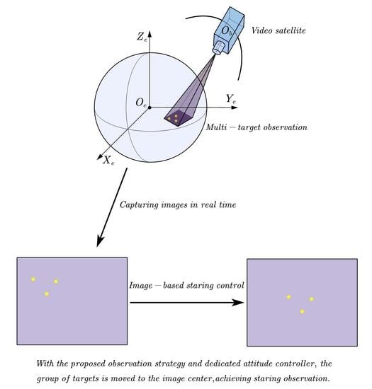Therefore, microsatellites (e.g., Skybox [1], LAPAN-TUBSAT [2], Tiantuo-2 [3] and so on) and CubeSats (e.g., HiREV [4] and Hera Constellation [5]) stand out in these video-based Earth observation missions. Using a staring attitude controller, a video satellite can constantly orient the space-borne camera towards the ground targets for a period of time when the satellite flies over the region of interest (ROI). In this way, video satellites are qualified for applications like disaster relief, ground surveillance, and so on. However, there are still challenges remaining unsolved. First, the staring control for a single target has been developed using different methods, but a dedicated controller for the scenario where multiple targets are to be observed has been missing. Second, in the presence of an uncalibrated camera, previous control methods are faced with a decline in pointing accuracy. In this paper, we propose an image-based adaptive staring controller that takes advantage of image information to achieve multi-target observation.

Staring control methods have been primarily based on the prior location information of the target, which we could call a position-based method. Since the ground target is fixed on the Earth’s surface, the location of the target to be observed can be acquired according to its longitude, latitude, and height. Also, the target’s velocity in the inertial frame is computed through Earth rotation. On the basis of the location, ref. [6] designs the desired attitude in both numerical and analytical ways and then proposes a PD-like staring controller to achieve the desired camera pointing. Ref. [7] proposes a slide-mode controller using a similar position-based attitude formulation. Ref. [8] generates staring control commands analytically for Earth observation satellite and compares different position-based staring control methods. It is worth noting that these staring controllers, including other applications in [9,10,11,12,13,14,15,16,17], deal with only a single target, thus are not adequate to properly observe a group of targets when they are in the field of view (FOV) simultaneously.

Compared with a single target observation task, observation for multiple targets is more complex. If the ground targets are distributed sparsely, the camera can capture only one target in one frame. If the targets are distributed densely, they can be seen in the FOV and recorded in one frame simultaneously. For the former observation case, Cui [18,19] considers targets located along the sub-satellite track, and adjusts the attitude of the satellite to stare at the ground targets consecutively. The observation is divided into two phases: the stable phase when observing one target and the transition phase when switching to the next target. Two different control methods are proposed. One [18] is a conventional PD-like controller but with variable coefficients in corresponding phases, and the other one [19] is an optimal controller that schedules the observation strategy. Similarly, ref. [20] studies a scheduling problem for aerial targets. Although multiple ground targets are considered in this scenario, the targets are distant from each other, hence only one target appears on the image at one time, and the multi-target observation is essentially transformed into a sequence of single-target observations. For the latter observation case, the way to solve the problem that the image contains more than one target at one time remains unclear, therefore we will propose our solution in this paper.

In practice, the placement and the structure of the camera can differ from the ideal conditions because of the vibration, thermal-induced influence, and other complex factors during the launch and in-orbit operation. Considering such an uncalibrated camera, no matter whether multiple targets are considered, the aforementioned position-based methods cannot avoid the pointing deviation because they are solely dependent on the location information of the target. Thus, an adaptive image-based staring controller is developed to overcome the drawbacks of those position-based methods.

To utilize the image information, the pixel coordinate of a target on the image should be first extracted. In fact, the state-of-art image processing techniques [21,22,23,24,25,26] have been constantly progressing to accomplish the target identification or tracking, and this paper attaches importance to the image-based control instead of image processing, i.e., we do not consider the image processing time. In staring imaging applications, ref. [27] proposes an image-based control algorithm but the image is only used to designate a vector to align with a ground vector, which is essentially still a position-based method. Ref. [28] realizes a staring controller whose attitude errors are derived from the image errors. The problem is that the camera in his method is assumed to be fully calibrated, which is quite difficult in reality. Both uncalibrated and calibrated cameras have been widely studied in robotics [29,30], UAVs [31,32] and many other engineering areas [33,34,35,36], but the dynamics considered in these works are different from those of a spacecraft, thus are not applicable to staring attitude control.

To sum up, some of the aforementioned studies are fully based on position, some only observe a single target, and some neglect the uncertainties of an uncalibrated camera. This paper deals with the situation where multiple targets appear on the image and the video satellite equipped with an uncalibrated camera is supposed to stare at these targets. First, we propose a selection strategy to designate two targets as representatives, and our controller is based on the two representatives rather than the whole set of targets. Second, we propose an image-based adaptive staring controller using parameter estimation, so that, even though the camera is uncalibrated, we can still accomplish the staring observation.

The paper is organized as follows. In Section 2, the projection model of a pin-hole camera is established. In Section 3, the multi-target observation problem is formulated based on the image-based kinematics. In Section 4, the selection strategy of the targets is introduced, and then we propose the adaptive controller, including the definition and estimation of parameters. Section 5 gives the simulation samples of the selection strategy and controller respectively. Conclusions are drawn in Section 6.

2. Camera Preliminaries

The ground target is projected onto the image plane and then recorded as pixels. This projection process is dependent on the camera’s internal structure, the camera’s external placement on the satellite, and the relative position between the satellite and the target. In this section, we analyze the parameters of a pin-hole camera that affect the projection by establishing the projection model from the target’s position in the inertial frame to its corresponding pixel coordinate on the image.

2.1. The Intrinsic Camera Model

The intrinsic camera model reflects the projection of the target point on the image plane, which is essentially a pinhole model and is shown in Figure 1. The focal length is denoted as f. $O-UV$ is the 2D pixel frame in the normalized image plane. $O_c-X_c{Y}_c{Z}_c$ is the camera coordinate system, where the axis $X_c$ and $Y_c$ is parallel with U and V respectively and $Z_c$ is perpendicular to the image plane with the point of intersection located at the center $\left(u_0,v_0\right)$. The position vector of the target is ${}^c{\mathit{R}}_{cT}={\left(x_c,y_c,z_c\right)}^T$, where the corner mark c shows that ${}^c{\mathit{R}}_{cT}$ is expressed in the camera frame, and the corresponding projection pixel coordinate is $\left(u,v\right)$. Suppose the pixel size is $dx\times dy$, then we have the following geometrical relation:

$$\frac{z_c}{f}=\frac{x_c}{\left(u-u_0\right)·dx}=\frac{y_c}{\left(v-v_0\right)·dy}$$

(1)

We can reorganize Equation (1) in the form of

$$z_c\left(\begin{array}{c}u\\ v\\ 1\end{array}\right)=\underset{\Pi }{\underbrace{\left(\begin{array}{ccc}f/dx& 0& \begin{array}{cc}{u}_0& 0\end{array}\\ 0& f/dy& \begin{array}{cc}{v}_0& 0\end{array}\\ 0& 0& \begin{array}{cc}1& 0\end{array}\end{array}\right)}}\left(\begin{array}{c}{x}_c\\ y_c\\ \begin{array}{c}{z}_c\\ 1\end{array}\end{array}\right)=\Pi \left(\begin{array}{c}{}^c{\mathit{R}}_{cT}\\ 1\end{array}\right)$$

(2)

where the matrix $\Pi$ contains the intrinsic camera parameters.

2.2. The Extrinsic Camera Model

The position and attitude of the camera frame with respect to the body frame, $O_c-X_c{Y}_c{Z}_c$, is displayed in Figure 2. ${}^c{\mathit{R}}_{bc}$ represents the position of $O_c$ in the camera frame. ${}^b{\mathit{R}}_{bT}$ is the target’s position in the body frame. ${}_b{}^{c}M$ represents the rotation matrix from the body frame to the camera frame. We define the homogeneous transform matrix from the body frame to the camera frame $T\in {\mathbb{R}}^{4\times 4}$:

$$T=\left(\begin{array}{cc}{}_b{}^{c}M& {-}^c{\mathit{R}}_{bc}\\ {\mathbf{0}}_{1\times 3}& 1\end{array}\right)$$

(3)

Then we have

$$\left(\begin{array}{c}{}^c{\mathit{R}}_{cT}\\ 1\end{array}\right)=T\left(\begin{array}{c}{}^b{\mathit{R}}_{bT}\\ 1\end{array}\right)$$

(4)

According to Equations (2) and (4), the target’s position in the satellite body frame can be transformed to the pixel coordinate by

$$\left(\begin{array}{c}u\\ v\\ 1\end{array}\right)=\frac{1}{z_c}\Pi ·T·\left(\begin{array}{c}{}^b{\mathit{R}}_{bT}\\ 1\end{array}\right)=\frac{1}{z_c}N\left(\begin{array}{c}{}^b{\mathit{R}}_{bT}\\ 1\end{array}\right)$$

(5)

where the projection matrix $N=\Pi ·T\in {\mathbb{R}}^{3\times 4}$. N contains all the camera-related parameters. In the remainder of the article, different combinations of elements of N are widely used in different mathematical expressions. For simplicity, we reorganize the 12 elements of matrix N as different submatrices. Let $n_{ij}$($i=1,2,3j=1,2,3,4$) represents the elements of the projection matrix N. Denote the first two rows of N as submatrix $\mathit{P}$, and the third row is submatrix ${\mathit{n}}_3^T$. And we further define the first three columns of $\mathit{P}$ as ${\mathit{P}}_{\left(3\right)}$ and the first three columns of ${\mathit{n}}_3^T$ as ${\mathit{n}}_{3\left(3\right)}^T$. Then we have the submatrices consisting of elements of N:

$$\begin{array}{cc}\hfill & \mathit{P}=\left(\begin{array}{c}\begin{array}{cccc}{n}_{11}& n_{12}& n_{13}& n_{14}\end{array}\\ \begin{array}{cccc}{n}_{21}& n_{22}& n_{23}& n_{24}\end{array}\end{array}\right),{\mathit{P}}_{\left(3\right)}=\left(\begin{array}{c}\begin{array}{ccc}{n}_{11}& n_{12}& n_{13}\end{array}\\ \begin{array}{ccc}{n}_{21}& n_{22}& n_{23}\end{array}\end{array}\right)\hfill \\ \hfill & {\mathit{n}}_3^T=\left(\begin{array}{cccc}{n}_{31}& n_{32}& n_{33}& n_{34}\end{array}\right),{\mathit{n}}_{3\left(3\right)}^T=\left(\begin{array}{ccc}{n}_{31}& n_{32}& n_{33}\end{array}\right)\hfill \\ \hfill & N=\left(\begin{array}{c}\mathit{P}\\ {\mathit{n}}_3^T\end{array}\right)\hfill \end{array}$$

(6)

2.3. Staring Observation for a Single Ground Target

In Figure 3, $O_e-X_e{Y}_e{Z}_e$ is the Earth-centered inertial (ECI) frame. Denote the rotation matrix from the ECI frame to the body frame as ${}_i{}^{b}M$. ${}^i{\mathit{R}}_{eb}$ represents the position vector from the Earth center to the satellite, which is expressed in the ECI frame. ${}^i{\mathit{R}}_{eT}$ is the position vector of the target in the ECI frame. Define the homogeneous transform matrix from the inertial frame to the body frame $T_h$:

$$T_h=\left(\begin{array}{cc}{}_i{}^{b}M& -{{}_i{}^{b}M}^i{\mathit{R}}_{eb}\\ {\mathbf{0}}_{1\times 3}& 1\end{array}\right)$$

(7)

Then the following equation is obtained:

$$\left(\begin{array}{c}{}^b{\mathit{R}}_{bT}\\ 1\end{array}\right)=T_h\left(\begin{array}{c}{}^i{\mathit{R}}_{eT}\\ 1\end{array}\right)$$

(8)

Substitute Equations (8) to (5), and we have the projection model:

$$\left(\begin{array}{c}u\\ v\\ 1\end{array}\right)=\frac{1}{z_c}N·T_h·\left(\begin{array}{c}{}^i{\mathit{R}}_{eT}\\ 1\end{array}\right)$$

(9)

Equation (9) shows the mapping relationship of the position of the target in the ECI frame and its pixel coordinate on the image. We define the pixel coordinate as $\mathit{y}\left(t\right)={\left(\begin{array}{cc}u\left(t\right)& v\left(t\right)\end{array}\right)}^T$, thus

$$\begin{array}{c}\hfill \mathit{y}=\frac{1}{z_c}\mathit{P}·T_h·\left(\begin{array}{c}{}^i{\mathit{R}}_{eT}\\ 1\end{array}\right)\\ \hfill z_c={\mathit{n}}_3^T·T_h·\left(\begin{array}{c}{}^i{\mathit{R}}_{eT}\\ 1\end{array}\right)\end{array}$$

(10)

where $\mathit{P}$ and ${\mathit{n}}_3^T$ are defined in Equation (6). For an uncalibrated camera, the camera parameters $\mathit{P}$ and ${\mathit{n}}_3^T$ are uncertain, therefore the estimation is needed.

3. Problem Formulation

This section first introduces the way to simplify the multi-target observation problem and then establishes the kinematics and dynamics of attitude motion in the form of pixel coordinates. In the end, the problem of a multi-target staring observation is formulated.

3.1. Multi-Target Observation

Assuming all the targets are contained in the FOV at the same time and hence can be detected on the image frame, we propose a strategy to observe the entirety of the targets properly. Like the example, in Figure 4a, the rectangle denotes the image borders, inside which there are 5 target points. For single-target observation, our staring objective is to control the only target to the image center. For a multi-target case, however, if we only consider a single target, this may lead to an unexpected result. Take Figure 4b as an example. Point 1 is moved to the image center but point 5 is lost in the FOV. And point 3 and 4 are far from the image center, which is not preferable either.

In light of this, we would prefer all the targets to be similarly distributed around the image center. One possible solution is to move the center of mass to the image center. Without loss of generality, we assume every point owns the same mass weight. Hence, for n targets whose pixel coordinates are denoted as ${\mathit{y}}_i$, $i=1,\cdots ,n$, the center of mass is given by

$$\mathit{\eta }\left(t\right)=\frac{1}{n}\sum _{i=1}^n{\mathit{y}}_i$$

(11)

The control objective is then to move $\mathit{\eta }\left(t\right)$ to the image center. However, a new problem arises in a situation where most target points are densely distributed in a small area while a few other points are far from this area. In this situation, $\mathit{\eta }\left(t\right)$ is almost the center of dense points, and our solution will finally place the dense points around the image center, from which the other points will be very far.

To realize the overall more balanced observation, we propose a selection strategy, which first classifies the target group into two clusters and then selects one target from each cluster, i.e., two targets in total. The center of mass $\mathit{\eta }\left(t\right)$ will be replaced by the midpoint of these two targets as our control object. In this way, two clusters are equally important and therefore have a similar distance from the image center. The details of this strategy will be further explained later.

3.2. Attitude Kinematics and Dynamics

The satellite in our study is regarded as a rigid body. Assume $\mathit{r}$ is the Euler axis from the ECI to the body frame and $\alpha$ is the rotation angle, then the attitude can be described by a quaternion $\mathit{q}={\left[q_0{\mathit{q}}_v\right]}^T$, which is defined as

$$\mathit{q}=cos\left(\alpha /2\right)+\mathit{r}sin\left(\alpha /2\right)=q_0+{\mathit{q}}_v$$

(12)

where $q_0$ is the scalar part and ${\mathit{q}}_v$ is the vector part of the quaternion, and the constraint $q_0^2+{\mathit{q}}_v^T{\mathit{q}}_v=1$ always holds. Let $\omega \left(t\right)$ be the angular velocity of the satellite with respect to the ECI frame expressed in the body frame, and we have the attitude kinematics given by

$$\begin{array}{cc}\hfill {\dot{q}}_0& =-\frac{1}{2}{\mathit{q}}_v^T\omega \hfill \\ \hfill {\dot{\mathit{q}}}_v& =\frac{1}{2}\left(q_0{E}_3+sk\left({\mathit{q}}_v\right)\right)\omega \hfill \end{array}$$

(13)

where $E_3$ is the $3\times 3$ identity matrix. For any 3-dimensional vector $\mathit{x}={\left[x_1,x_2,x_3\right]}^T$, the arithmetic operator $sk\left(·\right)$ is defined as

$$sk\left(\mathit{x}\right)=\left(\begin{array}{ccc}0& -x_3& x_2\\ x_3& 0& -x_1\\ -x_2& x_1& 0\end{array}\right)$$

(14)

The attitude dynamics of a rigid satellite are given by

$$J\dot{\omega }\left(t\right)=-\omega \left(t\right)\times J\omega \left(t\right)+\mathit{U}\left(t\right)$$

(15)

where J represents the inertia matrix of the satellite and $\mathit{U}\left(t\right)$ is the attitude control torques.

3.3. Projection Kinematics for a Single Point

Though the attitude of a satellite can be expressed in the form of a quaternion, instead of using an error quaternion like a conventional position-based method, our image-based method uses the error of the pixel coordinates to represent attitude error. Therefore, we need to figure out how the pixel coordinate varies with the angular velocity. Differentiate the depth $z_c\left(t\right)$ from Equation (10) and we get

$$\begin{array}{cc}\hfill {\dot{z}}_c\left(t\right)=& {\mathit{n}}_3^T\left(\begin{array}{cc}sk\left({}_i{}^{b}M{\left(t\right)}^i{\mathit{R}}_{eT}\left(t\right)-{}_i{}^{b}M{\left(t\right)}^i{\mathit{R}}_{eb}\left(t\right)\right)& -{}_i{}^{b}M\left(t\right)\\ {\mathbf{0}}_{1\times 3}& {\mathbf{0}}_{1\times 3}\end{array}\right)\left(\begin{array}{c}\omega \left(t\right)\\ {}^i{\mathit{V}}_{eb}\left(t\right)\end{array}\right)+{\mathit{n}}_3^T{T}_h\left(t\right)\left(\begin{array}{c}{}^i{\mathit{V}}_{eT}\left(t\right)\\ 0\end{array}\right)\hfill \\ \hfill =& {\mathit{n}}_{3\left(3\right)}^{T}sk\left({}_i{}^{b}M{\left(t\right)}^i{\mathit{R}}_{eT}\left(t\right)-{}_i{}^{b}M{\left(t\right)}^i{\mathit{R}}_{eb}\left(t\right)\right)\omega \left(t\right)+{\mathit{n}}_{3\left(3\right)}^T{}_i{}^{b}M\left(t\right)\left({}^i{\mathit{V}}_{eT}\left(t\right){-}^i{\mathit{V}}_{eb}\left(t\right)\right)\hfill \end{array}$$

(16)

where ${}^i{\mathit{V}}_{eT}$ is the velocity of the ground target and ${}^i{\mathit{V}}_{eb}$ is the velocity of the satellite. Similarly, the derivative of the image coordinate is given by

$$\begin{array}{cc}\hfill \dot{\mathit{y}}\left(t\right)=& \frac{1}{z_c\left(t\right)}\mathit{P}·{\dot{T}}_h\left(t\right)·\left(\begin{array}{c}{}^i{\mathit{R}}_{eT}\left(t\right)\\ 1\end{array}\right)-\frac{{\dot{z}}_c\left(t\right)}{z_c\left(t\right)}\mathit{y}\left(t\right)+\frac{1}{z_c\left(t\right)}\mathit{P}·T_h\left(t\right)·\left(\begin{array}{c}{}^i{\mathit{V}}_{eT}\left(t\right)\\ 1\end{array}\right)\hfill \\ \hfill =& \frac{1}{z_c\left(t\right)}\left[\left({\mathit{P}}_{\left(3\right)}-\mathit{y}\left(t\right){\mathit{n}}_{3\left(3\right)}^T\right)sk\left({}_i{}^{b}M{\left(t\right)}^i{\mathit{R}}_{eT}\left(t\right)-{}_i{}^{b}M{\left(t\right)}^i{\mathit{R}}_{eb}\left(t\right)\right)\omega \left(t\right)\right.\hfill \\ & +\left.\left({\mathit{P}}_{\left(3\right)}-\mathit{y}\left(t\right){\mathit{n}}_{3\left(3\right)}^T\right){}_i{}^{b}M\left(t\right)\left({}^i{\mathit{V}}_{eT}\left(t\right){-}^i{\mathit{V}}_{eb}\left(t\right)\right)\right]\hfill \end{array}$$

(17)

For simplicity, we define the matrix

$$\begin{array}{cc}\hfill a\left(t\right)=& {\mathit{n}}_{3\left(3\right)}^{T}sk\left({}_i{}^{b}M{\left(t\right)}^i{\mathit{R}}_{eT}\left(t\right)-{}_i{}^{b}M{\left(t\right)}^i{\mathit{R}}_{eb}\left(t\right)\right)\hfill \\ \hfill a_v\left(t\right)=& {\mathit{n}}_{3\left(3\right)}^T{}_i{}^{b}M\left(t\right)\left({}^i{\mathit{V}}_{eT}\left(t\right){-}^i{\mathit{V}}_{eb}\left(t\right)\right)\hfill \\ \hfill A\left(t\right)=& \left({\mathit{P}}_{\left(3\right)}-\mathit{y}\left(t\right){\mathit{n}}_{3\left(3\right)}^T\right)sk\left({}_i{}^{b}M{\left(t\right)}^i{\mathit{R}}_{eT}\left(t\right)-{}_i{}^{b}M{\left(t\right)}^i{\mathit{R}}_{eb}\left(t\right)\right)\hfill \\ \hfill A_v\left(t\right)=& \left({\mathit{P}}_{\left(3\right)}-\mathit{y}\left(t\right){\mathit{n}}_{3\left(3\right)}^T\right){}_i{}^{b}M\left(t\right)\left({}^i{\mathit{V}}_{eT}\left(t\right){-}^i{\mathit{V}}_{eb}\left(t\right)\right)\hfill \end{array}$$

(18)

Then Equations (16) and (17) can be rewritten as

$$\begin{array}{cc}\hfill {\dot{z}}_c\left(t\right)=& a\left(t\right)\omega \left(t\right)+a_v\left(t\right)\hfill \\ \hfill \dot{\mathit{y}}\left(t\right)=& \frac{1}{z_c\left(t\right)}\left(A\left(t\right)\omega \left(t\right)+A_v\left(t\right)\right)\hfill \end{array}$$

(19)

3.4. Projection Kinematics for Multiple Points

As we select two targets as the representatives of the entire group of targets, the kinematics of double target points should be derived. The center of mass of two targets is also their midpoint, which is

$$\mathit{\eta }\left(t\right)=\frac{1}{2}\left({\mathit{y}}_1\left(t\right)+{\mathit{y}}_2\left(t\right)\right)$$

(20)

where ${\mathit{y}}_1\left(t\right)$ and ${\mathit{y}}_2\left(t\right)$ are the two points respectively. The corner mark ${}_1$ and ${}_2$ are used to represent the two selected points in the remainder of this paper. Then we have

$$\begin{array}{cc}\hfill \frac{d\left(z_{c1}\left(t\right)·z_{c2}\left(t\right)\right)}{dt}=& \left(z_{c1}\left(t\right)a_2\left(t\right)+z_{c2}\left(t\right)a_1\left(t\right)\right)\omega \left(t\right)+\left(z_{c1}\left(t\right)a_{v2}\left(t\right)+z_{c2}\left(t\right)a_{v1}\left(t\right)\right)\hfill \\ \hfill =& h\left(t\right)\omega \left(t\right)+h_v\left(t\right)\hfill \end{array}$$

(21)

$$\begin{array}{cc}\hfill \dot{\mathit{\eta }}\left(t\right)=& \frac{1}{z_{c1}\left(t\right)·z_{c2}\left(t\right)}\left(\frac{z_{c2}\left(t\right)·A_1\left(t\right)+z_{c1}\left(t\right)·A_2\left(t\right)}{2}\omega \left(t\right)+\frac{z_{c2}\left(t\right)·A_{v1}\left(t\right)+z_{c1}\left(t\right)·A_{v2}\left(t\right)}{2}\right)\hfill \\ \hfill =& \frac{1}{z_{c1}\left(t\right)·z_{c2}\left(t\right)}\left(H\left(t\right)\omega \left(t\right)+H_v\left(t\right)\right)\hfill \end{array}$$

(22)

where

$$\begin{array}{cc}\hfill H\left(t\right)=& \frac{z_{c2}\left(t\right)·A_1\left(t\right)+z_{c1}\left(t\right)·A_2\left(t\right)}{2}\hfill \\ \hfill H_v\left(t\right)=& \frac{z_{c2}\left(t\right)·A_{v1}\left(t\right)+z_{c1}\left(t\right)·A_{v2}\left(t\right)}{2}\hfill \\ \hfill h\left(t\right)=& z_{c1}\left(t\right)a_2\left(t\right)+z_{c2}\left(t\right)a_1\left(t\right)\hfill \\ \hfill h_v\left(t\right)=& z_{c1}\left(t\right)a_{v2}\left(t\right)+z_{c2}\left(t\right)a_{v1}\left(t\right)\hfill \end{array}$$

(23)

Equations (21) and (22) are the dynamics of the midpoint of two targets. The way to select the two targets will be introduced in the next section.

3.5. Control Objective

At the initial time, a couple of ground targets are detected on the image through the space-borne camera. To acquire a better view of the entirety of the targets, we expect the center of mass of the target group to be located at the image center. In pursuit of a balanced observation, the midpoint $\mathit{\eta }\left(t\right)$ of two targets are picked out to best represent the group’s center of mass according to our proposed selection strategy. With a proper estimation of the camera-related parameters, our objective of the proposed adaptive controller is to move $\mathit{\eta }\left(t\right)$ to the image center, which is denoted as ${\mathit{\eta }}_d={\left(\begin{array}{cc}{u}_0& v_0\end{array}\right)}^T$.

4. Controller Design

In this section, the selection strategy is firstly introduced to find the two most suitable targets, which will then be used by the controller to achieve the control objective. As the camera is uncalibrated, the elements of the projection matrix N are unknown, hence the parameters to be estimated should be defined. Due to the fact that the ground point is constantly moving along with the Earth’s rotation, it is rather tough to determine the desired angular velocity when the target projection has reached ${\mathit{\eta }}_d$. Thus, a reference attitude trajectory will be proposed to avoid designing desired angular velocity in this section. And the adaptive staring controller will be designed based on the estimated parameters and the reference attitude.

4.1. Target-Selection Strategy Using a Clustering Method

Assuming there are targets denoted as ${\mathit{y}}_i$, $i=1,\cdots ,n$ on the image, we propose the following strategy to select two points to best serve our multi-target observation.

Step 1: We adopt a clustering algorithm, i.e., k-means [37], to classify all the targets into two clusters, e.g., $C_1$ and $C_2$. As a result, every point is classified as one of the two clusters and has the least distance from the center of mass of its corresponding cluster. Denote ${\mathit{c}}_1$ and ${\mathit{c}}_2$ as the center of mass of $C_1$ and $C_2$ respectively, then for any ${\mathit{y}}_j\in C_1$, we have

$$∥{\mathit{y}}_j-{\mathit{c}}_1∥⩽∥{\mathit{y}}_j-{\mathit{c}}_2∥$$

(24)

For any ${\mathit{y}}_k\in C_2$, we have

$$∥{\mathit{y}}_k-{\mathit{c}}_2∥⩽∥{\mathit{y}}_k-{\mathit{c}}_1∥$$

(25)

Step 2: We walk through all the target pairs consisting of two targets from the two clusters respectively. The target pair, of which the center of mass is closest to the center of mass of all the targets, is selected. Denote the selected targets as ${\mathit{y}}_1^{*}\in C_1$ and ${\mathit{y}}_2^{*}\in C_2$, and they satisfy

$$∥\frac{{\mathit{y}}_1^{*}+{\mathit{y}}_2^{*}}{2}-\frac{1}{n}\sum _{i=1}^n{\mathit{y}}_i∥=\underset{{\mathit{y}}_j\in C_1,{\mathit{y}}_k\in C_2}{min}∥\frac{{\mathit{y}}_j+{\mathit{y}}_k}{2}-\frac{1}{n}\sum _{i=1}^n{\mathit{y}}_i∥$$

(26)

Step 1 is to guarantee the balance of observation emphasis between two clusters, and step 2 is to find two proper targets whose midpoint resembles the center of mass of the entire target group most. Based on two selected targets, the following adaptive controller is designed to achieve the staring observation for multiple targets.

4.2. Parameter Definition

Due to the uncertainties of the uncalibrated camera, we have to properly define the camera parameters so that we can linearize and then estimate these parameters online. The parameter linearization is the basis of the parameter estimation and therefore we can formulate the adaptive controller using these estimated parameters. According to Equations (10) and (20), we have

$$\begin{array}{cc}\hfill 2z_{c1}\left(t\right)·z_{c2}\left(t\right)·\mathit{\eta }\left(t\right)=& z_{c2}\left(t\right)·\left(z_{c1}\left(t\right)·{\mathit{y}}_1\left(t\right)\right)+z_{c1}\left(t\right)·\left(z_{c2}\left(t\right)·{\mathit{y}}_2\left(t\right)\right)\hfill \\ \hfill =& z_{c2}\left(t\right)·\mathit{P}·T_h·\left(\begin{array}{c}{}^i{\mathit{R}}_{eT1}\\ 1\end{array}\right)+z_{c1}\left(t\right)·\mathit{P}·T_h·\left(\begin{array}{c}{}^i{\mathit{R}}_{eT2}\\ 1\end{array}\right)\hfill \end{array}$$

(27)

Each element of the projection matrix N appearing in the above equation is coupled with another element, i.e., they appear in the form of a product of two elements. We define these coupling products as the parameters $\theta$ to be estimated. More specifically, after Equation (27) is expanded, we can find that $\theta$ consists of the products of $n_{34}$ times every element of N, every element of ${\mathit{n}}_{3\left(3\right)}^T$ times every element of ${\mathit{n}}_{3\left(3\right)}^T$ and every element of ${\mathit{n}}_{3\left(3\right)}^T$ times every element of $\mathit{P}$. Hence $\theta$ contains 42 parameters. As we can infer, the number of the parameters defined will fast increase when dealing with the center of mass of over two targets. In other words, the parameter estimation process will be more complex and computationally demanding. Therefore, our target-selection strategy is also able to reduce the computational burden.

The estimated values of the parameters are denoted as $\widehat{\theta }\left(t\right)$, and the head mark $\widehat{}$ is used to represent the estimated variables in the remainder of this paper.

4.3. Reference Attitude Trajectory

A PD-like controller requires the convergence of both the image error $\Delta \mathit{\eta }\left(t\right)=\mathit{\eta }\left(t\right)-{\mathit{\eta }}_d$ and the angular velocity error ${\omega }_e\left(t\right)=\omega \left(t\right)-{\omega }_d\left(t\right)$. But the time-varying desired angular velocity ${\omega }_d\left(t\right)$ is hard to directly design. To avoid using ${\omega }_d\left(t\right)$, we propose the reference attitude. In this way, the attitude of the satellite is controlled to track the reference attitude instead. Define a reference trajectory of the midpoint as ${\mathit{\eta }}_r\left(t\right)$:

$${\dot{\mathit{\eta }}}_r\left(t\right)={\dot{\mathit{\eta }}}_d-\lambda \Delta \mathit{\eta }\left(t\right)=-\lambda \Delta \mathit{\eta }\left(t\right)$$

(28)

The reference angular velocity trajectory ${\omega }_r\left(t\right)$ is defined as

$${\omega }_r\left(t\right)={\widehat{H}}^{+}\left(t\right)\left(-{\widehat{z}}_{c1}\left(t\right){\widehat{z}}_{c2}\left(t\right)·\lambda ·\Delta \mathit{\eta }\left(t\right)-{\widehat{H}}_v\left(t\right)\right)$$

(29)

where the pseudo inverse matrix ${\widehat{H}}^{+}\left(t\right)$ of $\widehat{H}\left(t\right)$ is defined as

$$\begin{array}{cc}\hfill {\delta }_{\dot{\mathit{\eta }}}\left(t\right)=& \dot{\mathit{\eta }}\left(t\right)-{\dot{\mathit{\eta }}}_r\left(t\right)=\Delta \dot{\mathit{\eta }}\left(t\right)+\lambda \Delta \mathit{\eta }\left(t\right)\hfill \\ \hfill {\delta }_{\omega }\left(t\right)=& \omega \left(t\right)-{\omega }_r\left(t\right)\hfill \end{array}$$

(30)

${\delta }_{\dot{\mathit{\eta }}}\left(t\right)$ and ${\delta }_{\omega }\left(t\right)$ reflect the tracking error between the current attitude and the reference attitude. Worth noting that, the convergence of ${\delta }_{\dot{\mathit{\eta }}}\left(t\right)$ infers the convergence of $\Delta \mathit{\eta }\left(t\right)$, which, according to its definition, is mathematically obvious and hence no proof is listed here.

4.4. Parameter Estimation

The estimation error is defined as $\Delta \theta \left(t\right)=\widehat{\theta }\left(t\right)-\theta$. According to Equation (27), an estimated projection error $\mathit{e}\left(t\right)$ used to measure the performance of the parameter estimation is given by

$$\begin{array}{cc}\hfill \mathit{e}\left(t\right)=& 2{\widehat{z}}_{c1}\left(t\right)·{\widehat{z}}_{c2}\left(t\right)·\mathit{\eta }\left(t\right)-{\widehat{z}}_{c1}\left(t\right)·\widehat{\mathit{P}}·T_h·\left(\begin{array}{c}{}^i{\mathit{R}}_{eT2}\\ 1\end{array}\right)-{\widehat{z}}_{c2}\left(t\right)·\widehat{\mathit{P}}·T_h·\left(\begin{array}{c}{}^i{\mathit{R}}_{eT1}\\ 1\end{array}\right)\hfill \\ \hfill =& W\left(t\right)·\Delta \theta \left(t\right)\hfill \end{array}$$

(31)

The matrix $W\left(t\right)$ does not contain any camera parameters. Due to the proper definition of parameters, $\mathit{e}\left(t\right)$ is linear with respect to $\Delta \theta \left(t\right)$, which enables us to estimate the parameters. Accordingly, we propose an updating law for the parameters $\widehat{\theta }\left(t\right)$:

$$\dot{\widehat{\theta }}\left(t\right)=-{\Gamma }^{-1}\left\{Y^T\left(t\right){\delta }_{\dot{\mathit{\eta }}}\left(t\right)+W^T\left(t\right)K_1\mathit{e}\left(t\right)\right\}$$

(32)

where the regressor matrix $Y\left(t\right)$ is given by

$$\begin{array}{cc}\hfill \Delta {\theta }^T\left(t\right)·Y^T\left(t\right)=& -\left[\left(z_{c1}\left(t\right)z_{c2}\left(t\right)-{\widehat{z}}_{c1}\left(t\right){\widehat{z}}_{c2}\left(t\right)\right){\dot{\mathit{\eta }}}_r\left(t\right)-\left(H_v\left(t\right)-{\widehat{H}}_v\left(t\right)\right)\right.\hfill \\ & {\left.-\left(H\left(t\right)-\widehat{H}\left(t\right)\right)\omega \left(t\right)\right]}^T{K}_2\hfill \end{array}$$

(33)

$K_1$ and $K_2$ are the diagonal positive coefficient matrices, and $Y\left(t\right)$ does not contain any camera parameters. The updating law (32) contains two main parts. The first part will be utilized in the stability proof, and the second is about the negative gradient of $\mathit{e}\left(t\right)$, which updates the parameters in a direction that $\mathit{e}\left(t\right)$ is reducing.

4.5. Adaptive Staring Controller

The adaptive staring controller is given by

$$\mathit{U}\left(t\right)=\omega \left(t\right)\times J\omega \left(t\right)+J{\dot{\omega }}_r\left(t\right)-K_3{\delta }_{\omega }\left(t\right)-{\widehat{H}}^T\left(t\right)K_2{\delta }_{\dot{\mathit{\eta }}}\left(t\right)$$

(34)

where $\mathit{U}\left(t\right)$ is the attitude control torque, $K_2$ and $K_3$ are the diagonal positive coefficient matrices. Define two non-negative function

$$\begin{array}{cc}\hfill V_1\left(t\right)=& \frac{1}{2}{\delta }_{\omega }^T\left(t\right)J{\delta }_{\omega }\left(t\right)\hfill \\ \hfill V_2\left(t\right)=& \frac{1}{2}\Delta {\theta }^T\left(t\right)\Gamma \Delta \theta \left(t\right)\hfill \end{array}$$

(35)

Then we have the Lyapunov function $V\left(t\right)=V_1\left(t\right)+V_2\left(t\right)$. Differentiate $V_1\left(t\right)$:

$$\begin{array}{cc}\hfill {\dot{V}}_1\left(t\right)=& {\delta }_{\omega }^T\left(t\right)J{\dot{\delta }}_{\omega }\left(t\right)\hfill \\ \hfill =& {\delta }_{\omega }^T\left(t\right)J\left(\dot{\omega }\left(t\right)-{\dot{\omega }}_r\left(t\right)\right)\hfill \\ \hfill =& {\delta }_{\omega }^T\left(t\right)\left(-\omega \left(t\right)\times J\omega \left(t\right)+\mathit{U}\left(t\right)-J{\dot{\omega }}_r\left(t\right)\right)\hfill \\ \hfill =& {\delta }_{\omega }^T\left(t\right)\left(-K_3{\delta }_{\omega }\left(t\right)-{\widehat{H}}^T{\left(t\right)}^T\left(t\right)K_2{\delta }_{\dot{\mathit{\eta }}}\left(t\right)\right)\hfill \\ \hfill =& -{\delta }_{\omega }^T\left(t\right)K_3{\delta }_{\omega }\left(t\right)-{\delta }_{\omega }^T\left(t\right){\widehat{H}}^T\left(t\right)K_2{\delta }_{\dot{\mathit{\eta }}}\left(t\right)\hfill \end{array}$$

(36)

Differentiate $V_2\left(t\right)$:

$$\begin{array}{cc}\hfill {\dot{V}}_2\left(t\right)=& \Delta {\theta }^T\left(t\right)\Gamma \Delta \dot{\theta }\left(t\right)\hfill \\ \hfill =& -\Delta {\theta }^T\left(t\right)\left\{Y^T\left(t\right){\delta }_{\dot{\mathit{\eta }}}\left(t\right)+W^T\left(t\right)K_1\mathit{e}\left(t\right)\right\}\hfill \\ \hfill =& -\Delta {\theta }^T\left(t\right)Y^T\left(t\right){\delta }_{\dot{\mathit{\eta }}}\left(t\right)-{\mathit{e}}^T\left(t\right)K_1\mathit{e}\left(t\right)\hfill \end{array}$$

(37)

We rewrite $V_1\left(t\right)$ and $V_2\left(t\right)$:

$$\begin{array}{cc}\hfill {\omega }^T\left(t\right){\widehat{H}}^T\left(t\right)=& {\omega }^T\left(t\right)H^T\left(t\right)+{\omega }^T\left(t\right)\left({\widehat{H}}^T\left(t\right)-H^T\left(t\right)\right)\hfill \\ \hfill =& {\left[z_{c1}\left(t\right)z_{c2}\left(t\right)\dot{\mathit{\eta }}\left(t\right)-H_v\left(t\right)\right]}^T+{\omega }^T\left(t\right)\left({\widehat{H}}^T\left(t\right)-H^T\left(t\right)\right)\hfill \\ \hfill =& {\left[z_{c1}\left(t\right)z_{c2}\left(t\right){\dot{\mathit{\eta }}}_r\left(t\right)-H_v\left(t\right)+z_{c1}\left(t\right)z_{c2}\left(t\right)\left(\dot{\mathit{\eta }}\left(t\right)-{\dot{\mathit{\eta }}}_r\left(t\right)\right)\right]}^T\hfill \\ & +{\omega }^T\left(t\right)\left({\widehat{H}}^T\left(t\right)-H^T\left(t\right)\right)\hfill \\ \hfill =& {\left[z_{c1}\left(t\right)z_{c2}\left(t\right){\dot{\mathit{\eta }}}_r\left(t\right)-H_v\left(t\right)+z_{c1}\left(t\right)z_{c2}\left(t\right){\delta }_{\dot{\mathit{\eta }}}\left(t\right)\right]}^T\hfill \\ & +{\omega }^T\left(t\right)\left({\widehat{H}}^T\left(t\right)-H^T\left(t\right)\right)\hfill \\ \hfill {\omega }_r^T\left(t\right){\widehat{H}}^T\left(t\right)=& {\left[{\widehat{z}}_{c1}\left(t\right){\widehat{z}}_{c2}\left(t\right){\dot{\mathit{\eta }}}_r\left(t\right)-{\widehat{H}}_v\left(t\right)\right]}^T\hfill \end{array}$$

(38)

Simultaneously, we have

$${\delta }_{\omega }^T\left(t\right){\widehat{H}}^T\left(t\right)={\omega }^T\left(t\right){\widehat{H}}^T\left(t\right)-{\omega }_r^T\left(t\right){\widehat{H}}^T\left(t\right)$$

(39)

The ${\delta }_{\omega }^T\left(t\right){\widehat{H}}^T\left(t\right)K_2{\delta }_{\dot{\mathit{\eta }}}\left(t\right)$ part in Equation (36) can then be rewritten as

$$\begin{array}{cc}\hfill {\delta }_{\omega }^T\left(t\right){\widehat{H}}^T\left(t\right)K_2{\delta }_{\dot{\mathit{\eta }}}\left(t\right)=& \left[\left(z_{c1}\left(t\right)z_{c2}\left(t\right)-{\widehat{z}}_{c1}\left(t\right){\widehat{z}}_{c2}\left(t\right)\right){\dot{\mathit{\eta }}}_r\left(t\right)-\left(H_v\left(t\right)-{\widehat{H}}_v\left(t\right)\right)\right.\hfill \\ & {\left.-\left(H\left(t\right)-\widehat{H}\left(t\right)\right)\omega \left(t\right)\right]}^T{K}_2{\delta }_{\dot{\mathit{\eta }}}\left(t\right)+z_{c1}\left(t\right)z_{c2}\left(t\right){\delta }_{\dot{\mathit{\eta }}}^T\left(t\right)K_2{\delta }_{\dot{\mathit{\eta }}}\left(t\right)\hfill \\ \hfill =& z_{c1}\left(t\right)z_{c2}\left(t\right){\delta }_{\dot{\mathit{\eta }}}^T\left(t\right)K_2{\delta }_{\dot{\mathit{\eta }}}\left(t\right)-\Delta {\theta }^T\left(t\right)·Y^T\left(t\right)·{\delta }_{\dot{\mathit{\eta }}}\left(t\right)\hfill \end{array}$$

(40)

Substitute Equations (38)–(40) into (36) and (37), and the following inequality is obtained

$$\begin{array}{cc}\hfill \dot{V}\left(t\right)=& {\dot{V}}_1\left(t\right)+{\dot{V}}_2\left(t\right)\hfill \\ \hfill =& -{\delta }_{\omega }^T\left(t\right)K_3{\delta }_{\omega }\left(t\right)-z_{c1}\left(t\right)z_{c2}\left(t\right){\delta }_{\dot{\mathit{\eta }}}^T\left(t\right)K_2{\delta }_{\dot{\mathit{\eta }}}\left(t\right)-{\mathit{e}}^T\left(t\right)K_1\mathit{e}\left(t\right)\hfill \\ \hfill ⩽& 0\hfill \end{array}$$

(41)

We can conclude that $\omega \left(t\right)$, $\mathit{e}\left(t\right)$ and $\widehat{\theta }\left(t\right)$ are all bounded, which leads to the control torque $\mathit{U}\left(t\right)$ also being bounded. According to the dynamics Equation (15), $\dot{\omega }\left(t\right)$ is bounded. Considering the expression of $\dot{\mathit{e}}\left(t\right)$ and $\dot{\widehat{\theta }}\left(t\right)$, they are bounded, too. Therefore, we have the boundedness of $\ddot{V}\left(t\right)$. According to Barbalat’s Lemma, the following convergence is obtained

$$\begin{array}{cc}\hfill \underset{t\to \infty }{lim}{\delta }_{\omega }\left(t\right)=& \mathbf{0}\hfill \\ \hfill \underset{t\to \infty }{lim}{\delta }_{\dot{\mathit{\eta }}}\left(t\right)=& \mathbf{0}\hfill \\ \hfill \underset{t\to \infty }{lim}\mathit{e}\left(t\right)=& \mathbf{0}\hfill \end{array}$$

(42)

which suggests that

$$\begin{array}{cc}\hfill \underset{t\to \infty }{lim}\Delta \mathit{\eta }\left(t\right)=& \mathbf{0}\hfill \\ \hfill \underset{t\to \infty }{lim}\Delta \dot{\mathit{\eta }}\left(t\right)=& \mathbf{0}\hfill \end{array}$$

(43)

Hence the stability of the proposed adaptive staring controller is proved. The midpoint of two ground targets’ projections on the image plane is moved to the image center under the effect of our controller.

5. Simulations

This section presents the simulation results of our proposed target selection method and adaptive staring controller. With an emphasis on the staring control, our simulations do not consider the image processing time and assume the pixel coordinates of the target point on the image are obtained in real-time.

5.1. Target Selection

Two cases are tested to assess the performance of the target selection method. Each case has a different number and distribution of target points on the image.

Table 1. Distribution of targets.

Targets	Case 1	Case 2
Point 1	(60; 400)	(480; 70)
Point 2	(100; 500)	(550; 40)
Point 3	(200; 350)	(620; 280)
Point 4	(220; 400)	(700; 120)
Point 5	(150; 300)	(610; 90)
Point 6	∖	(590; 300)
Point 7	∖	(650; 80)

lists the pixel coordinates of all the target points. Five points located mainly in the left-top area of the image are tested in Case 1, and seven points located mainly in the right-bottom area of the image are tested in Case 2.

The results of the proposed selecting method are shown in Figure 5. In both cases, the targets are divided into two clusters according to their relative locations. Every point has the least distance to the center of mass of its corresponding cluster. From each cluster respectively, a target, marked by a circle or rhombus in Figure 5, is selected to form a target pair. The midpoint of these two target points resembles the center of mass of the entire target group most.

5.2. Staring Control

In an ideal condition, the values of the camera parameters equal the ideal values, which are listed in

Table 2. Camera parameters.

Camera Parameters	Theoretical Values	Real Values
f	1 m	1.1 m
$u_0$	376	396
$v_0$	291	276
$dx\&dy$	$8.33\times {10}^{-6}$ m	$8.43\times {10}^{-6}$
${}^c{\mathit{R}}_{bc}$	$\left(\begin{array}{c}-0.2682\\ 0.0408\\ 0.0671\end{array}\right)$ m	$\left(\begin{array}{c}-0.2582\\ 0.0358\\ 0.0771\end{array}\right)$ m
${}_b{}^{c}M$	$M_{321}\left(-{30}^{\circ },{40}^{\circ },-{20}^{\circ }\right)$	$M_{321}\left(-{29}^{\circ },39.6^{\circ },-18.9^{\circ }\right)$

. The operation $M_{321}\left(·\right)$ is the rotation matrix representing a 3-2-1 rotation sequence. However, the camera used on the satellite is uncalibrated, therefore the unknown real values of the camera parameters are different from their ideal values. The image is comprised of $752\times 582$ pixels with the center $\left(376,291\right)$.

At the initial time (12 July 2021 04:30:00 UTC), a group of ground targets appears on the image, and then we conduct the proposed control to accomplish the staring observation. The first step is to select two targets out of the entire set. And the second step is to control the midpoint of the two selected targets to the image center. Without considering the height, the geographic locations of the ground targets are shown in

Table 3. Locations of ground targets.

	Target 1	Target 2	Target 3	Target 4	Target 5
Longitude (${}^{\circ }$)	128.279	128.262	128.261	128.271	128.271
Latitude (${}^{\circ }$)	64.71	64.725	64.717	64.715	64.72

. In

Table 4. Initial attitude.

Quaternion q	Angular Velocity $\mathit{\omega }{(}^{\circ }/\mathit{s})$
${\left(0.1795,-0.7553,0.6211,0.1077\right)}^T$	${\left(-3.0997,10,-2.9061\right)}^T\times {10}^{-4}$

, the initial attitude is given. In

Table 5. Initial orbital elements.

Semi-Major Axis	Eccentricity	Inclination	Argument of Perigee	RAAN	True Anomaly
6868.14 km	0	97.2574${}^{\circ }$	59.3884${}^{\circ }$	290.017${}^{\circ }$	54.8163${}^{\circ }$

where the right ascension of the ascending node is abbreviated to RAAN, we list the initial orbital elements, indicating an approximately 500 km high sun-synchronous orbit is adopted.

The maximum control torque of each axis is bounded by $U_{max}$ in

Table 6. Satellite parameters.

J	${\mathit{U}}_{\mathit{max}}$
$\left(\begin{array}{ccc}2.2240& -0.03264& 0.02083\\ -0.03264& 3.2550& -0.007557\\ 0.02083& -0.07557& 2.1922\end{array}\right)$ kg·m${}^2$	0.1 N·m

. In our simulations, the inertia matrix J of the satellite is also given in Table 6 and the proposed controller adopts the control parameters in

Table 7. Control parameters.

Parameter	Value
$K_1$	$2\times E_3\times {10}^{-15}$
$K_2$	$\left(\begin{array}{cc}3& 0\\ 0& 1\end{array}\right)\times {10}^{-21}$
$K_3$	$1.1\times E_3$
$\Gamma$	$\mathrm{diag}\left\{E_7\times {10}^5,8\times {10}^{-2},2\times E_{10}\times {10}^{14},8\times E_{16}\times {10}^8,4\times E_8\times {10}^8\right\}$

, where $\mathrm{diag}\left\{·\right\}$ represents a matrix with all the inputs placed at the diagonal. With the conditions listed in these tables, the simulation is conducted at a step size of 0.1s in the control loop.

Before the controller gets involved, we conduct target selection and the result is shown in Figure 6. At the initial time, there are overall five targets appearing on the image, and they are mainly located at the left bottom part. Two targets are picked out according to our selection strategy. Based on the selected two targets, the control torques are calculated and the attitude is adjusted accordingly, thus the projections of targets on the image are also moving. Figure 7 depicts the trajectories of the selected targets and their midpoint. The initial locations are marked by a circle while the final ones are marked by a square. As our controller takes effect, the targets start to move along the trajectories, reach the final locations and eventually converge to the final locations. The midpoint, as is shown, is kept at the image center $\left(376,291\right)$. The shape of the trajectory indicates that the target is not directly converging to its desired location in the initial stage, instead, it gradually adjusts the direction of its movement and finally turns to the final location. This is because there exists relative angular motion between the ground target and the optical axis of the camera according to initial conditions listed in Table 3, Table 4 and Table 5. In the initial stage, the initial relative motion is the dominant factor affecting the trajectory. As the controller gradually reorientates the camera to the target, the trajectory will eventually reach the desired destination. Although our controller is established on the two targets, Figure 8 shows that the observation for the entirety of five targets is also achieved at the same time, thanks to the proper selection of two representatives. Comparing Figure 6 with Figure 8, we can see the target points are all distributed around the image center with well-proportioned distances, therefore we can obtain the overall balanced observation for the whole group of targets in the field of view.

Figure 9 shows the estimated projection error $\mathit{e}\left(t\right)$ defined in Equation (31). Although the actual parameters are unknown, the proposed parameter estimating method (32) is constantly updating the parameters in a direction of the negative gradient of $\mathit{e}\left(t\right)$, thus $\mathit{e}\left(t\right)$ are reduced, which indicates that the estimated projection of the target on the image is approaching the actual projection. Our adaptive controller is formed on the basis of these estimated parameters, therefore the constant updating of parameters contributes to controlling the projection to the correct and desired location. The evolutions of angular velocity and control torques are shown in Figure 10 and Figure 11 respectively. The angular velocity experiences a rapid acceleration at the starting phase. This is because current angular motion needs to catch up with the desired motion so that the targets will not drift out of the field view. Accordingly, the control torques are outputted to support the angular acceleration. Soon after the rapid adjustment of angular motion, the angular velocity reaches a relatively stable phase. During this phase, the midpoint of the selected targets are gradually converging to the image center, and the rotation of the satellite is mainly to follow the motion of ground targets, which is actually the Earth rotation. Due to no need to conduct fast angular acceleration at this phase, the control torque outputs also decrease to a very low level. Even though we have moved the targets to the desired locations during the stable phase, it is worth noting that the angular velocity and control torques are quite small but not zero. Since the relative motion between the satellite and the Earth’s rotation is always time-varying, it is always required to adjust the angular motion to some extent. Only in this way, the staring observation can be maintained.

6. Conclusions

In light of the lack of a staring control method for a multi-target observation scenario, especially for an uncalibrated camera of a miniaturized video satellite, we propose an image-based adaptive staring controller. First, a selection strategy based on a clustering method is proposed and two targets as representatives are picked out of the entirety of the targets, which realizes a more balanced overall observation and also reduces the computational complexity. Second, the unknown camera parameters are estimated according to the self-updating law. As a result, the estimated projection error decreases. Third, the image-based adaptive staring controller for multiple targets is established using the estimated parameters. The simulations demonstrate the effectiveness of our proposed method. In the test case, though the camera is uncalibrated, our controller accomplishes the staring observation for a group of targets on the image.

In this paper, the motion of ground targets is predictable due to Earth’s rotation. For targets with unpredictable motion, a dedicated staring controller remains to be developed in the future.

References

1. d’Angelo, P.; Máttyus, G.; Reinartz, P. Skybox image and video product evaluation. Int. J. Image Data Fusion 2016, 7, 3–18. [Google Scholar] [CrossRef]
2. Julzarika, A. Utilization of LAPAN Satellite (TUBSAT, A2, and A3) in supporting Indonesia’s potential as maritime center of the world. In Proceedings of the IOP Conference Series: Earth and Environmental Science; IOP Publishing: Philadelphia, PA, USA, 2017; Volume 54, p. 012097. [Google Scholar]
3. Zhang, X.; Xiang, J.; Zhang, Y. Space object detection in video satellite images using motion information. Int. J. Aerosp. Eng. 2017, 2017, 1024529. [Google Scholar] [CrossRef]
4. Cho, D.H.; Choi, W.S.; Kim, M.K.; Kim, J.H.; Sim, E.; Kim, H.D. High-resolution image and video CubeSat (HiREV): Development of space technology test platform using a low-cost CubeSat platform. Int. J. Aerosp. Eng. 2019, 2019, 8916416. [Google Scholar] [CrossRef]
5. Poghosyan, A.; Golkar, A. CubeSat evolution: Analyzing CubeSat capabilities for conducting science missions. Prog. Aerosp. Sci. 2017, 88, 59–83. [Google Scholar] [CrossRef]
6. Lian, Y.; Gao, Y.; Zeng, G. Staring imaging attitude control of small satellites. J. Guid. Control. Dyn. 2017, 40, 1278–1285. [Google Scholar] [CrossRef]
7. Wu, S.; Sun, X.; Sun, Z.; Wu, X. Sliding-mode control for staring-mode spacecraft using a disturbance observer. Proc. Inst. Mech. Eng. Part G J. Aerosp. Eng. 2010, 224, 215–224. [Google Scholar] [CrossRef]
8. Han, S.; Ahn, J.; Tahk, M.J. Analytical Staring Attitude Control Command Generation Method for Earth Observation Satellites. J. Guid. Control. Dyn. 2022, 45, 1–10. [Google Scholar] [CrossRef]
9. Li, H.; Zhao, Y.; Li, B.; Li, G. Attitude Control of Staring-Imaging Satellite Using Permanent Magnet Momentum Exchange Sphere. In Proceedings of the 2019 22nd International Conference on Electrical Machines and Systems (ICEMS), Harbin, China, 11–14 August 2019; pp. 1–6. [Google Scholar]
10. Li, C.; Geng, Y.; Guo, Y.; Han, P. Suboptimal Repointing Maneuver of a staring-mode spacecraft with one DOF for final attitude. Acta Astronaut. 2020, 175, 349–361. [Google Scholar] [CrossRef]
11. Chen, X.; Ma, Y.; Geng, Y.; Wang, F.; Ye, D. Staring imaging attitude tracking control of agile small satellite. In Proceedings of the 2011 6th IEEE Conference on Industrial Electronics and Applications, Beijing, China, 21–23 June 2011; pp. 143–148. [Google Scholar]
12. Li, P.; Dong, Y.; Li, H. Staring Imaging Real-Time Optimal Control Based on Neural Network. Int. J. Aerosp. Eng. 2020, 2020, 8822223. [Google Scholar] [CrossRef]
13. Zhang, F.; Jin, L.; Rodrigo, G.A. An innovative satellite sunlight-reflection staring attitude control with angular velocity constraint. Aerosp. Sci. Technol. 2020, 103, 105905. [Google Scholar] [CrossRef]
14. Lian, Y.; Meng, Y.; Zheng, W. Multi-reference Decentralized Cooperative Satellite Attitude Control for Ground-Target Staring. In Proceedings of the International Conference on Autonomous Unmanned Systems; Springer: Berlin/Heidelberg, Germany, 2021; pp. 2193–2202. [Google Scholar]
15. Geng, Y.; Li, C.; Guo, Y.; Biggs, J.D. Hybrid robust and optimal control for pointing a staring-mode spacecraft. Aerosp. Sci. Technol. 2020, 105, 105959. [Google Scholar] [CrossRef]
16. Song, C.; Fan, C.; Song, H.; Wang, M. Spacecraft Staring Attitude Control for Ground Targets Using an Uncalibrated Camera. Aerospace 2022, 9, 283. [Google Scholar] [CrossRef]
17. Wu, Y.H.; Han, F.; Zheng, M.H.; Wang, F.; Hua, B.; Chen, Z.M.; Cheng, Y.H. Attitude tracking control for a space moving target with high dynamic performance using hybrid actuator. Aerosp. Sci. Technol. 2018, 78, 102–117. [Google Scholar] [CrossRef]
18. Cui, K.K.; Xiang, J.H. Variable coefficients pd adaptive attitude control of video satellite for ground multi-object staring imaging. In Proceedings of the Electrical Engineering and Automation: Proceedings of the International Conference on Electrical Engineering and Automation (EEA2016); World Scientific: Singapore, 2017; pp. 738–750. [Google Scholar]
19. Cui, K.; Xiang, J.; Zhang, Y. Mission planning optimization of video satellite for ground multi-object staring imaging. Adv. Space Res. 2018, 61, 1476–1489. [Google Scholar] [CrossRef]
20. Yu, Y.; Hou, Q.; Zhang, J.; Zhang, W. Mission scheduling optimization of multi-optical satellites for multi-aerial targets staring surveillance. J. Frankl. Inst. 2020, 357, 8657–8677. [Google Scholar] [CrossRef]
21. Said, Y.; Saidani, T.; Smach, F.; Atri, M.; Snoussi, H. Embedded real-time video processing system on FPGA. In Proceedings of the International Conference on Image and Signal Processing; Springer: Berlin/Heidelberg, Germany, 2012; pp. 85–92. [Google Scholar]
22. Ghodhbani, R.; Horrigue, L.; Saidani, T.; Atri, M. Fast FPGA prototyping based real-time image and video processing with high-level synthesis. Int. J. Adv. Comput. Sci. Appl. 2020, 11, 108–116. [Google Scholar] [CrossRef]
23. Qi, B.; Shi, H.; Zhuang, Y.; Chen, H.; Chen, L. On-board, real-time preprocessing system for optical remote-sensing imagery. Sensors 2018, 18, 1328. [Google Scholar] [CrossRef]
24. Yu, S.; Yuanbo, Y.; He, X.; Lu, M.; Wang, P.; An, X.; Fang, X. On-Board Fast and Intelligent Perception of Ships With the “Jilin-1” Spectrum 01/02 Satellites. IEEE Access 2020, 8, 48005–48014. [Google Scholar] [CrossRef]
25. Du, B.; Cai, S.; Wu, C. Object tracking in satellite videos based on a multiframe optical flow tracker. IEEE J. Sel. Top. Appl. Earth Obs. Remote Sens. 2019, 12, 3043–3055. [Google Scholar] [CrossRef]
26. Zhang, X.; Xiang, J. Moving object detection in video satellite image based on deep learning. In Proceedings of the LIDAR Imaging Detection and Target Recognition 2017; SPIE: Bellingham, WA, USA, 2017; Volume 10605, pp. 1149–1156. [Google Scholar]
27. Zdešar, A.; Klančar, G.; Mušič, G.; Matko, D.; Škrjanc, I. Design of the image-based satellite attitude control algorithm. In Proceedings of the 2013 XXIV International Conference on Information, Communication and Automation Technologies (ICAT), Sarajevo, Bosnia and Herzegovina, 30 October–1 November 2013; pp. 1–8. [Google Scholar]
28. Zhang, X.Y.; Xiang, J.H. Tracking imaging feedback attitude control of video satellite. In Proceedings of the Electrical Engineering and Automation: Proceedings of the International Conference on Electrical Engineering and Automation (EEA2016); World Scientific: Singapore, 2017; pp. 729–737. [Google Scholar]
29. Liu, Y.H.; Wang, H.; Wang, C.; Lam, K.K. Uncalibrated visual servoing of robots using a depth-independent interaction matrix. IEEE Trans. Robot. 2006, 22, 804–817. [Google Scholar]
30. Wang, H.; Liu, Y.H.; Zhou, D. Adaptive visual servoing using point and line features with an uncalibrated eye-in-hand camera. IEEE Trans. Robot. 2008, 24, 843–857. [Google Scholar] [CrossRef]
31. Gonzalez-Garcia, A.; Miranda-Moya, A.; Castañeda, H. Robust visual tracking control based on adaptive sliding mode strategy: Quadrotor UAV-catamaran USV heterogeneous system. In Proceedings of the 2021 International Conference on Unmanned Aircraft Systems (ICUAS), Athens, Greece, 15–18 June 2021; pp. 666–672. [Google Scholar]
32. Xie, H.; Lynch, A.F.; Low, K.H.; Mao, S. Adaptive output-feedback image-based visual servoing for quadrotor unmanned aerial vehicles. IEEE Trans. Control. Syst. Technol. 2019, 28, 1034–1041. [Google Scholar] [CrossRef]
33. Fan, C.; Liu, Y.; Song, B.; Zhou, D. Dynamic visual servoing of a small scale autonomous helicopter in uncalibrated environments. Sci. China Inf. Sci. 2011, 54, 1855–1867. [Google Scholar] [CrossRef]
34. Qiu, Z.; Hu, S.; Liang, X. Disturbance observer based adaptive model predictive control for uncalibrated visual servoing in constrained environments. ISA Trans. 2020, 106, 40–50. [Google Scholar] [CrossRef]
35. Felicetti, L.; Emami, M.R. Image-based attitude maneuvers for space debris tracking. Aerosp. Sci. Technol. 2018, 76, 58–71. [Google Scholar] [CrossRef]
36. Pesce, V.; Opromolla, R.; Sarno, S.; Lavagna, M.; Grassi, M. Autonomous relative navigation around uncooperative spacecraft based on a single camera. Aerosp. Sci. Technol. 2019, 84, 1070–1080. [Google Scholar] [CrossRef]
37. MacQueen, J. Classification and analysis of multivariate observations. In Proceedings of the 5th Berkeley Symposium on Mathematical Statistics and Probability; Statistical Laboratory of the University of California: Berkeley, CA, USA, 1967; pp. 281–297. [Google Scholar]
Figure 1. The intrinsic camera model.
Remotesensing 14 03974 g001
Figure 2. The extrinsic camera model.
Remotesensing 14 03974 g002
Figure 3. Staring observation for a single ground target.
Remotesensing 14 03974 g003
Figure 4. Staring observation for multiple ground targets. (a) Initial point distribution. (b) Inappropriate point distribution.
Remotesensing 14 03974 g004
Figure 5. Target selection results of case 1 (a) and case 2 (b).
Remotesensing 14 03974 g005
Figure 6. The initial target distribution and selection results.
Remotesensing 14 03974 g006
Figure 7. The trajectories of the two selected targets and their midpoint.
Remotesensing 14 03974 g007
Figure 8. The final target distribution.
Remotesensing 14 03974 g008
Figure 9. The time histories of estimated projection error.
Remotesensing 14 03974 g009
Figure 10. The time histories of angular velocity.
Remotesensing 14 03974 g010
Figure 11. The time histories of control torques.
Remotesensing 14 03974 g011