
Detection of Oil Spills in the Northern South China Sea Using Landsat-8 OLI

 ,
,  ,
,
Abstract
:
1. Introduction
2. Data
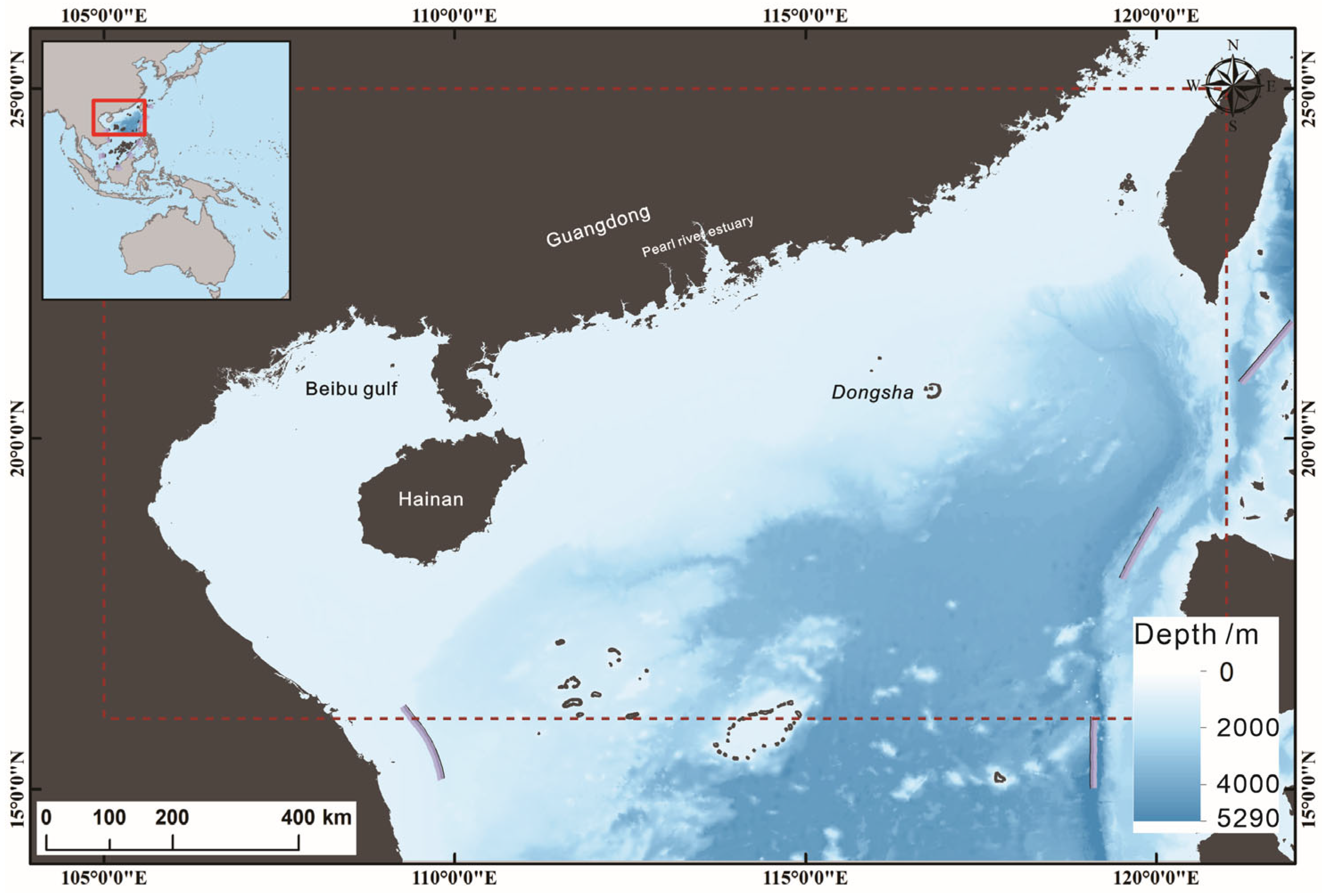
2.1. Study Area
2.2. Satellite Datasets
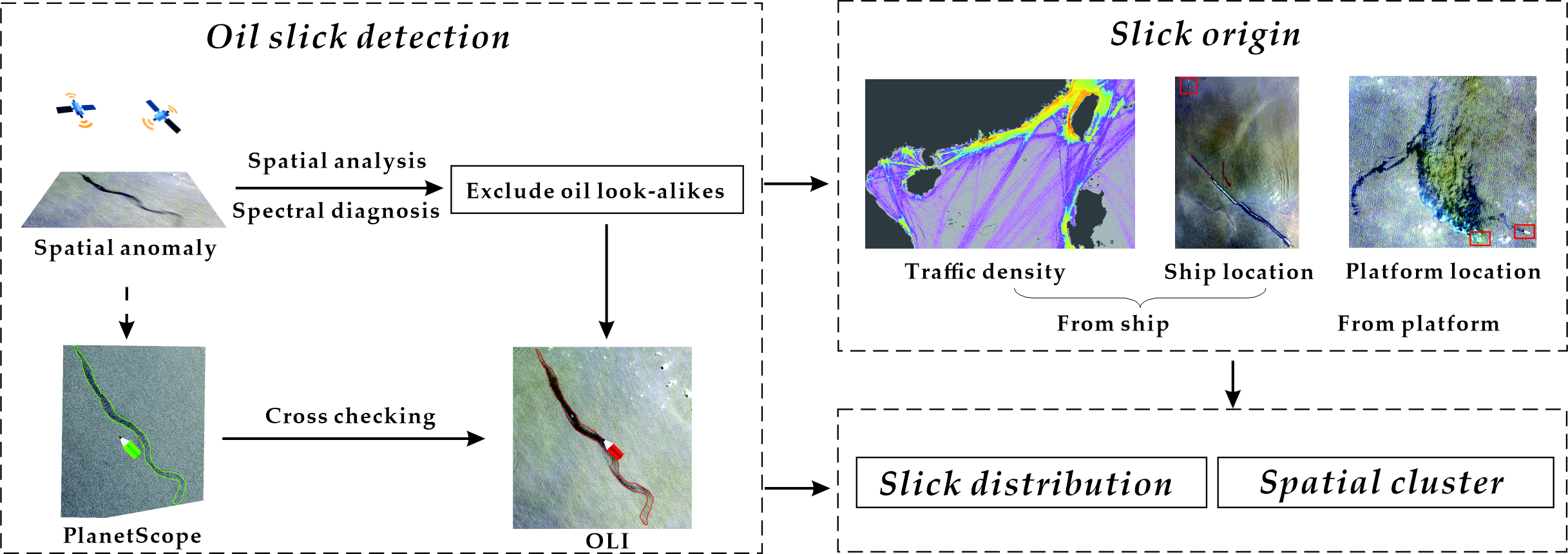
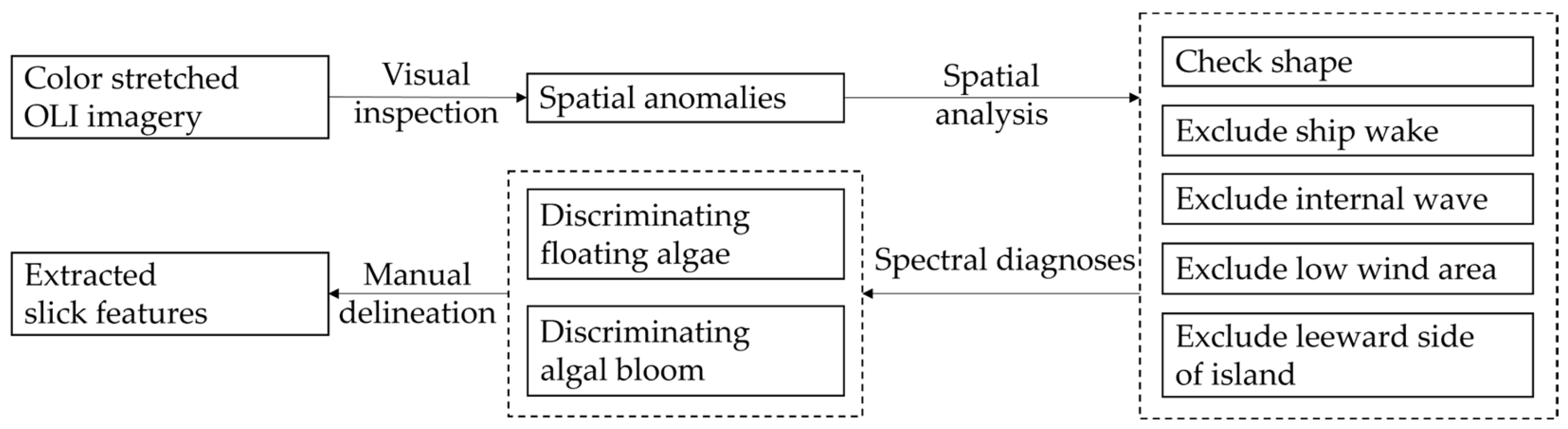
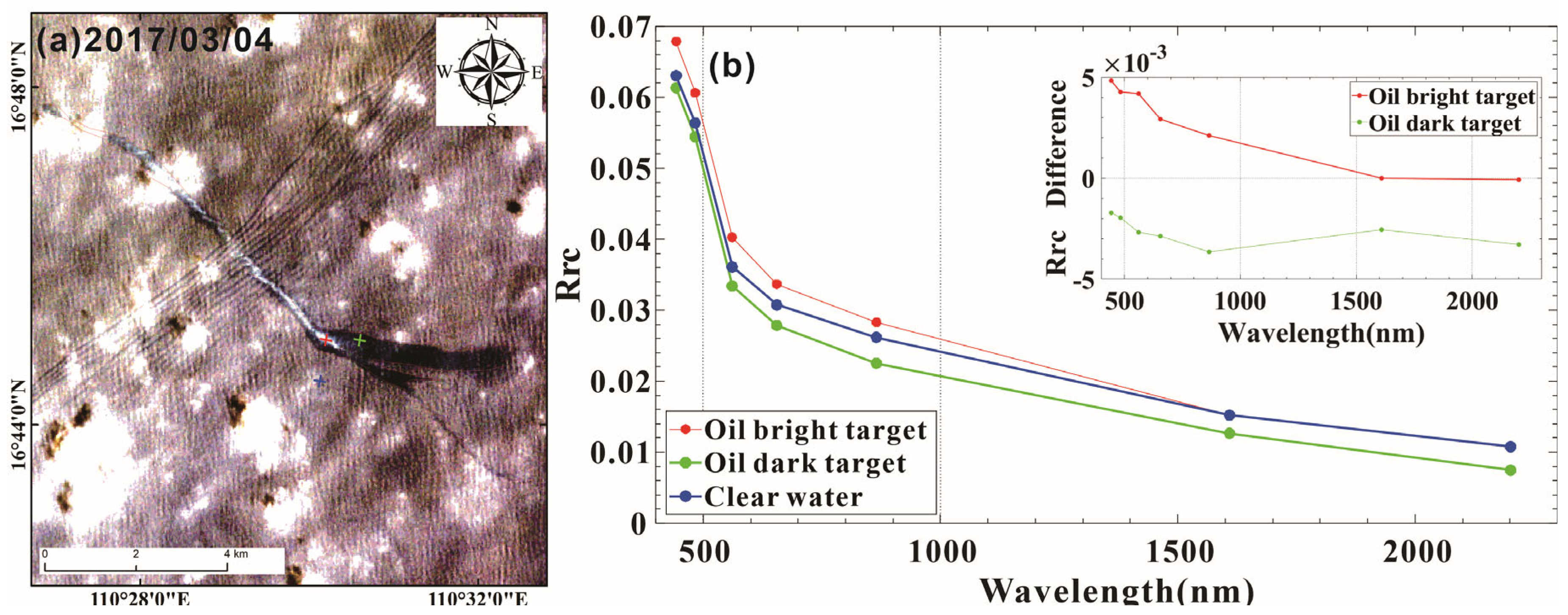
2.3. Oil Slick Detection by OLI
2.4. Offshore Platform Database and Traffic Densities
3. Results
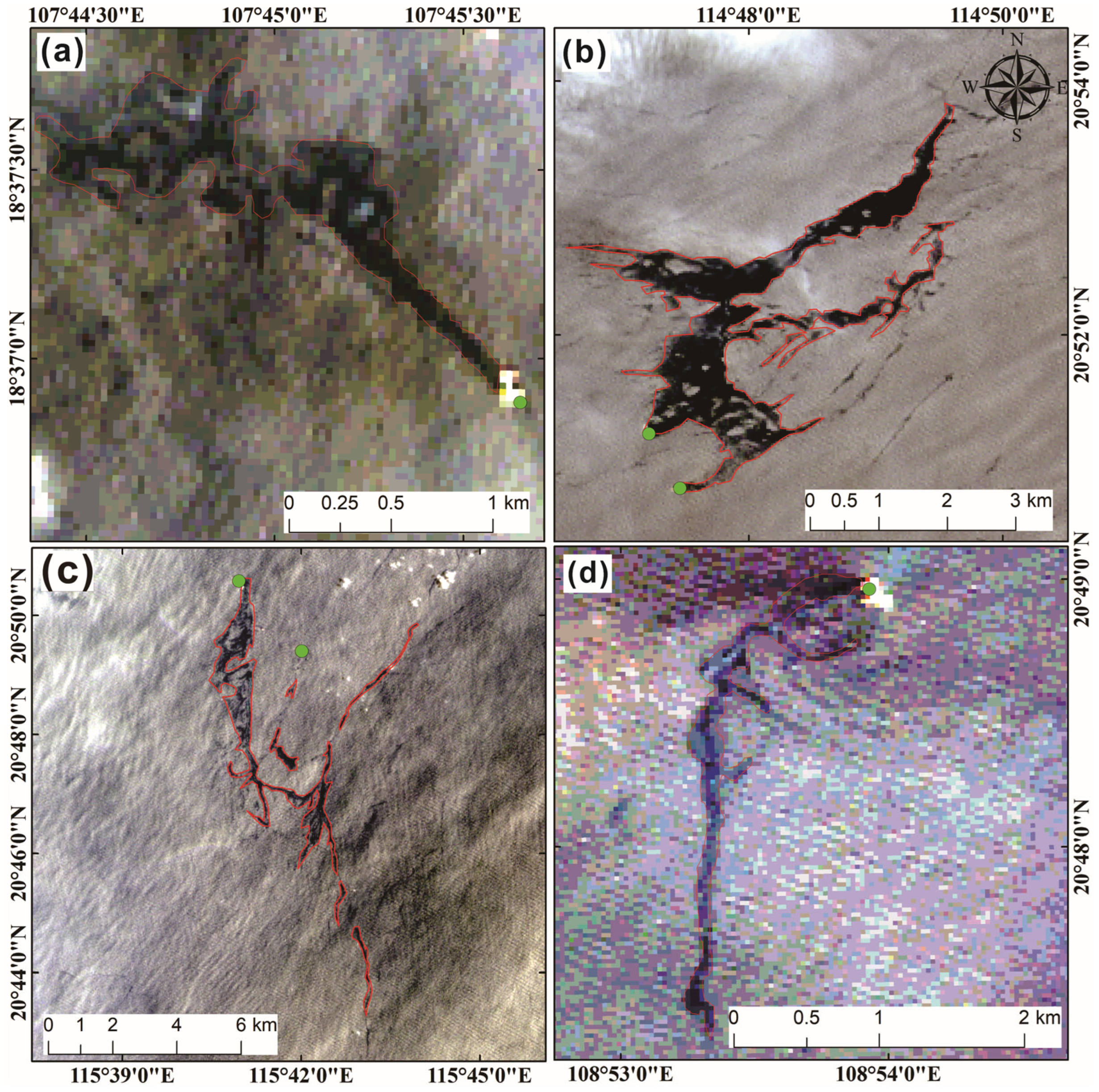
3.1. Delineated Oil Slicks
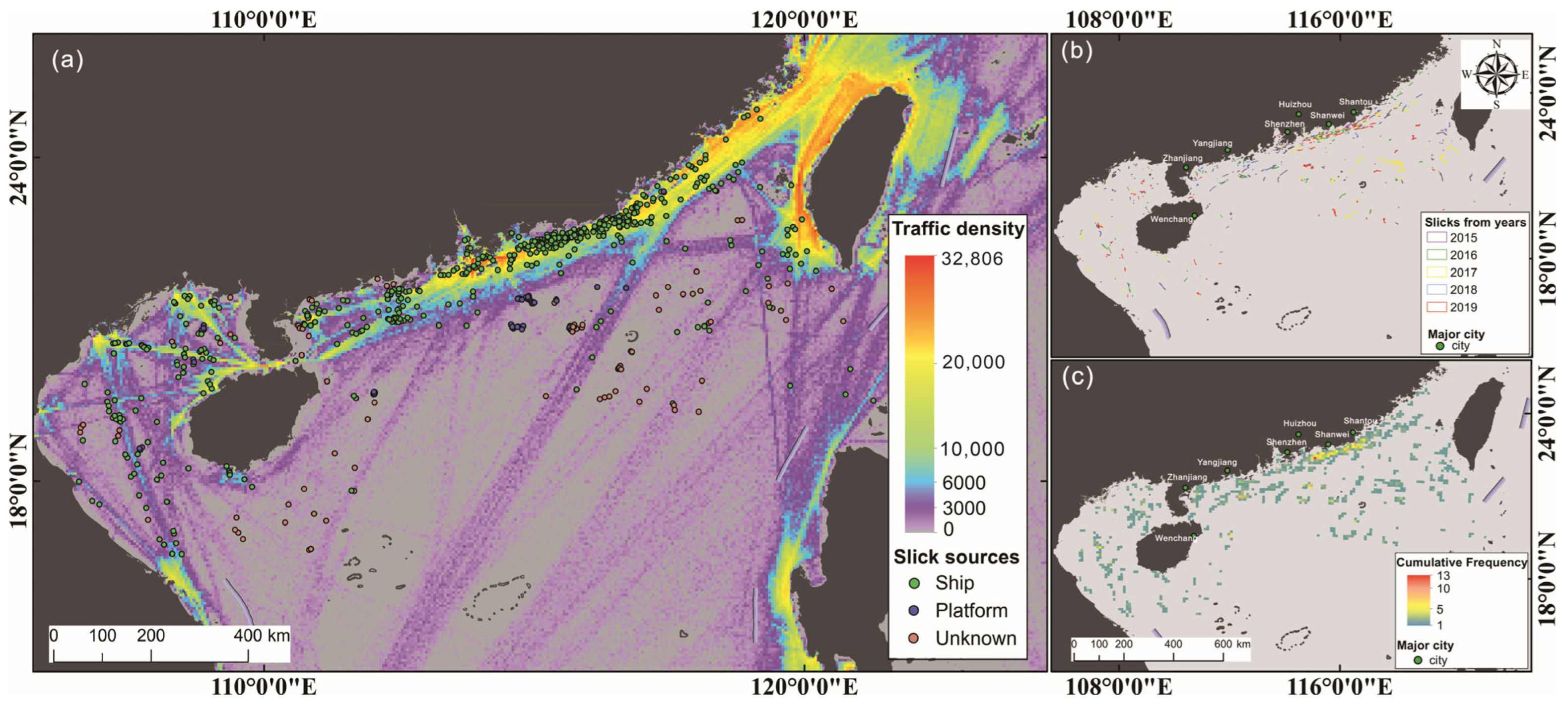
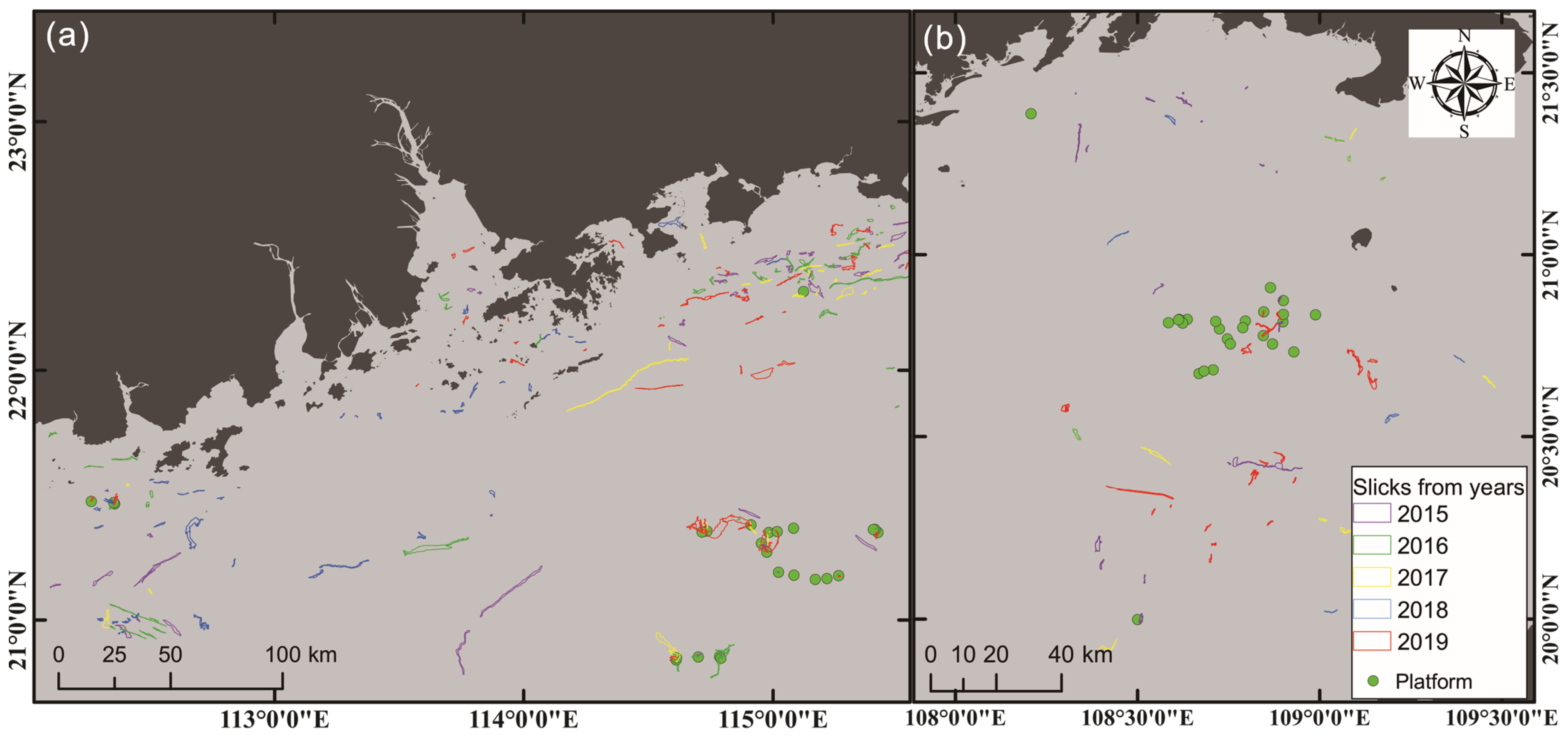
3.2. Distribution of Oil Spills
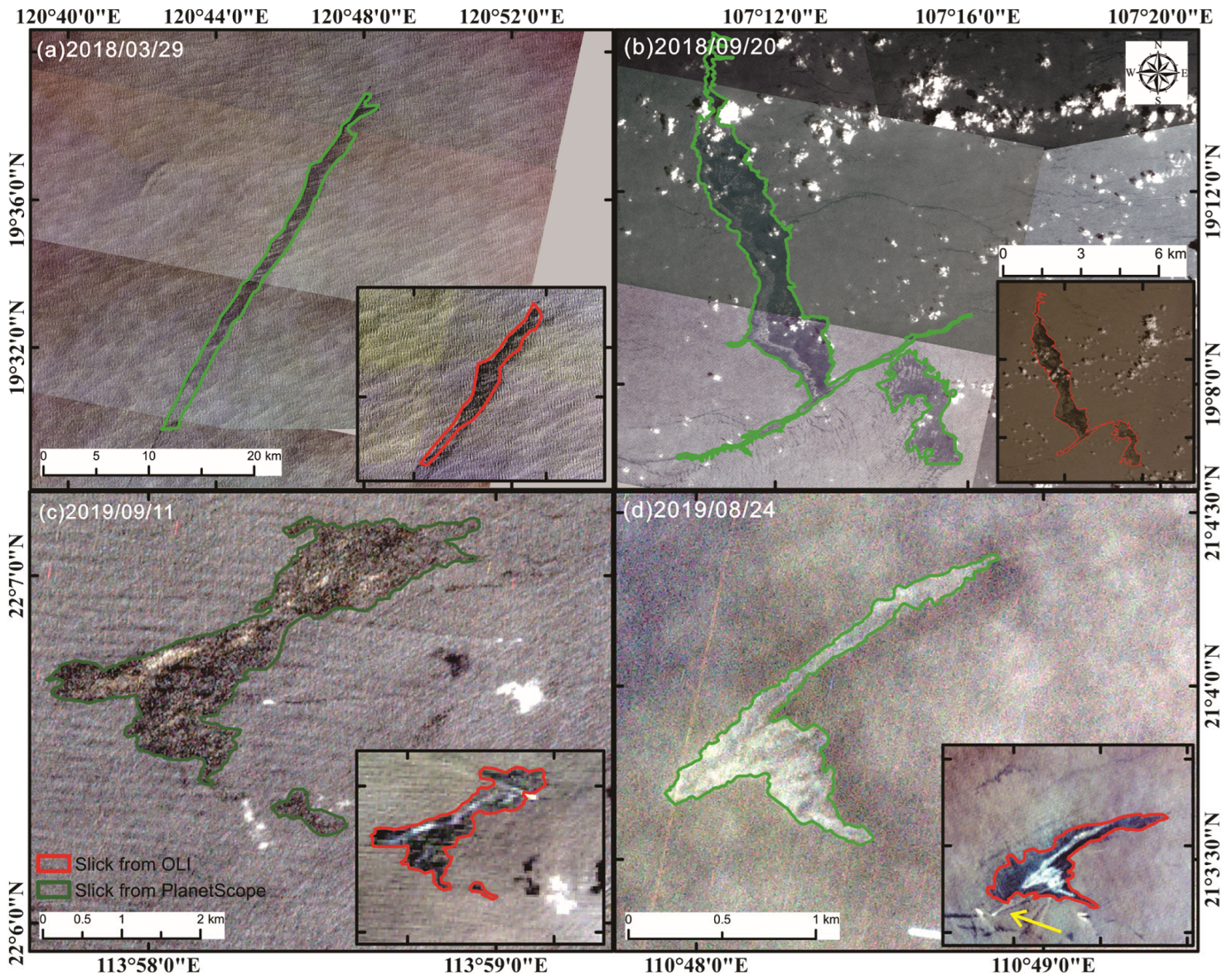
3.3. Cross-Check
4. Discussion
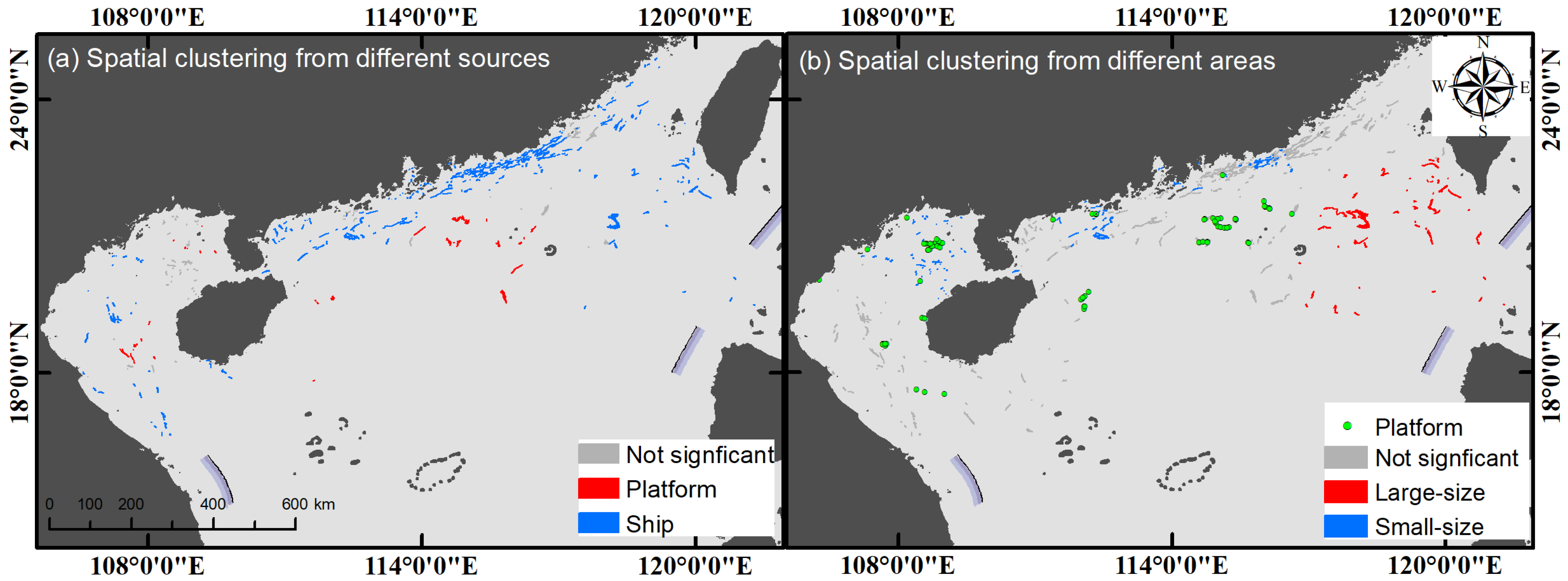
4.1. Slick Distribution from Different Sources
4.2. Uncertainties
5. Conclusions
Supplementary Materials
Author Contributions
Funding
Data Availability Statement
Acknowledgments
Conflicts of Interest
References
- DOINews. DOINews: Scientific Teams Refine Estimates of Oil Flow from BP’s Well Prior to Capping; U.S. Department of the Interior: Washington, DC, USA, 2010; Volume 2022.
- Sun, S.; Lu, Y.; Liu, Y.; Wang, M.; Hu, C. Tracking an oil tanker collision and spilled oils in the East China Sea using multisensor day and night satellite imagery. Geophys. Res. Lett. 2018, 45, 3212–3220. [Google Scholar] [CrossRef]
- Hebbar, A.A.; Dharmasiri, I.G. Management of marine oil spills: A case study of the Wakashio oil spill in Mauritius using a lens-actor-focus conceptual framework. Ocean Coast. Manag. 2022, 221, 106103. [Google Scholar] [CrossRef]
- International Tanker Owners Pollution Federation (ITOPF). Oil Tanker Spill Statistics 2021. Available online: https://www.itopf.org/knowledge-resources/data-statistics/statistics (accessed on 11 July 2022).
- National Research Council (US). Oil in the Sea III: Inputs, Fates, and Effects; National Academies Press (US): Washington, DC, USA, 2003. [Google Scholar]
- Fingas, M. The Basic of Oil Spill Clean Up, 3rd ed.; CRC Press: Boca Raton, FL, USA, 2012. [Google Scholar]
- Dong, Y.; Liu, Y.; Hu, C.; MacDonald, I.R.; Lu, Y. Chronic oiling in global oceans. Science 2022, 376, 1300–1304. [Google Scholar] [CrossRef] [PubMed]
- Laffon, B.; Pásaro, E.; Valdiglesias, V. Effects of exposure to oil spills on human health: Updated review. J. Toxicol. Environ. Health Part B Crit. Rev. 2016, 19, 105–128. [Google Scholar] [CrossRef] [PubMed]
- Keramea, P.; Spanoudaki, K.; Zodiatis, G.; Gikas, G.; Sylaios, G. Oil spill modeling: A critical review on current trends, perspectives, and challenges. J. Mar. Sci. Eng. 2021, 9, 181. [Google Scholar] [CrossRef]
- U.S. Environmental Protection Agency (EPA). Oil Discharge Reporting Requirements. Available online: https://www.epa.gov/sites/default/files/2014-06/documents/spccfactsheetspillreportingdec06-1.pdf (accessed on 11 July 2022).
- Daneshgar Asl, S.; Amos, J.; Woods, P.; Garcia-Pineda, O.; MacDonald, I.R. Chronic, anthropogenic hydrocarbon discharges in the Gulf of Mexico. Deep Sea Res. Part II Top. Stud. Oceanogr. 2016, 129, 187–195. [Google Scholar] [CrossRef]
- Chen, Q.; Hu, S. Study on offshore oil spill accidents in China. Mar. Dev. Manag. 2020, 37, 49–53. [Google Scholar]
- Gong, Y.; Zhao, P.; Lan, D.; Zhu, R.; Yan, X.U.; Bao, C.; Chunyan, Y.U. Characteristics and trend analysis of marine oil spill accidents in China. Ocean Dev. Manag. 2018, 35, 42–45. [Google Scholar]
- Brekke, C.; Solberg, A. Oil spill detection by satellite remote sensing. Remote Sens. Environ. 2005, 95, 1–13. [Google Scholar] [CrossRef]
- Fingas, M.; Brown, C. Review of oil spill remote sensing. Mar. Pollut. Bull. 2014, 83, 9–23. [Google Scholar] [CrossRef]
- Leifer, I.; Lehr, W.J.; Simecek-Beatty, D.; Bradley, E.; Clark, R.; Dennison, P.; Hu, Y.; Matheson, S.; Jones, C.E.; Holt, B.; et al. State of the art satellite and airborne marine oil spill remote sensing: Application to the BP Deepwater Horizon oil spill. Remote Sens. Environ. 2012, 124, 185–209. [Google Scholar] [CrossRef]
- Kokaly, R.F.; Couvillion, B.R.; Holloway, J.; Roberts, D.A.; Ustin, S.L.; Peterson, S.H.; Khanna, S.; Piazza, S.C. Spectroscopic remote sensing of the distribution and persistence of oil from the Deepwater Horizon spill in Barataria Bay marshes. Remote Sens. Environ. 2013, 129, 210–230. [Google Scholar] [CrossRef]
- Lu, Y.; Zhan, W.; Hu, C. Detecting and quantifying oil slick thickness by thermal remote sensing: A ground-based experiment. Remote Sens. Environ. 2016, 181, 207–217. [Google Scholar] [CrossRef]
- Garcia-Pineda, O.; MacDonald, I.; Hu, C.; Svejkovsky, J.; Hess, M.; Dukhovskoy, D.; Morey, S.L. Detection of floating oil anomalies from the Deepwater Horizon oil spill with synthetic aperture radar. Oceanography 2013, 26, 124–137. [Google Scholar] [CrossRef]
- Mohr, V.; Gade, M. Marine oil pollution in an area of high economic use: Statistical analyses of SAR data from the Western Java Sea. Remote Sens. 2022, 14, 880. [Google Scholar] [CrossRef]
- Trinadha Rao, V.; Suneel, V.; Raajvanshi, I.; Alex, M.J.; Thomas, A.P. Year-to-year variability of oil pollution along the Eastern Arabian Sea: The impact of COVID-19 imposed lock-downs. Mar. Pollut. Bull. 2022, 175, 113356. [Google Scholar] [CrossRef]
- Garcia-Pineda, O.; MacDonald, I.R.; Li, X.; Jackson, C.R.; Pichel, W.G. Oil spill mapping and measurement in the Gulf of Mexico with Textural Classifier Neural Network Algorithm (TCNNA). IEEE J. Sel. Top. Appl. Earth Obs. Remote Sens. 2013, 6, 2517–2525. [Google Scholar] [CrossRef]
- Hu, C.; Weisberg, R.H.; Liu, Y.; Zheng, L.; Daly, K.L.; English, D.C.; Zhao, J.; Vargo, G.A. Did the northeastern Gulf of Mexico become greener after the Deepwater Horizon oil spill? Geophys. Res. Lett. 2011, 38, L09601. [Google Scholar] [CrossRef]
- Hu, C.; Li, X.; Pichel, W.G.; Muller-Karger, F.E. Detection of natural oil slicks in the NW Gulf of Mexico using MODIS imagery. Geophys. Res. Lett. 2009, 36, L1604. [Google Scholar] [CrossRef]
- Sun, S.; Hu, C.; Garcia-Pineda, O.; Kourafalou, V.; Le Hénaff, M.; Androulidakis, Y. Remote sensing assessment of oil spills near a damaged platform in the Gulf of Mexico. Mar. Pollut. Bull. 2018, 136, 141–151. [Google Scholar] [CrossRef]
- Chen, T. Study on rapid prediction of oil spill drift in the east of the South China Sea. China Pet. Chem. Stand. Qual. 2020, 5, 168–172. [Google Scholar]
- Chang, P.; Yang, Q. Necessity and feasibility of establishing a particularly sensitive sea area system in the South China Sea. Water Transp. Manag. 2018, 15, 6–8. [Google Scholar]
- Vanhellemont, Q. Adaptation of the dark spectrum fitting atmospheric correction for aquatic applications of the Landsat and Sentinel-2 archives. Remote Sens. Environ. 2019, 225, 175–192. [Google Scholar] [CrossRef]
- Planet Team. Planet Team. Planet Application Program Interface. In Space for Life on Earth; Planet Team: San Francisco, CA, USA, 2017; Available online: https://api.planet.com (accessed on 11 July 2022).
- Sun, S.; Hu, C. The challenges of interpreting oil–water spatial and spectral contrasts for the estimation of oil thickness: Examples from satellite and airborne measurements of the Deepwater Horizon oil spill. IEEE Trans. Geosci. Remote 2019, 57, 2643–2658. [Google Scholar] [CrossRef]
- Sun, S.; Hu, C. Sun glint requirement for the remote detection of surface oil films. Geophys. Res. Lett. 2016, 43, 309–316. [Google Scholar] [CrossRef]
- Sun, S.; Hu, C.; Feng, L.; Swayze, G.A.; Holmes, J.; Graettinger, G.; Macdonald, I.; Garcia, O.; Leifer, I. Oil slick morphology derived from AVIRIS measurements of the Deepwater Horizon oil spill: Implications for spatial resolution requirements of remote sensors. Mar. Pollut. Bull. 2016, 103, 276–285. [Google Scholar] [CrossRef]
- Liu, Y.; Zhao, J.; Qin, Y. A novel technique for ship wake detection from optical images. Remote Sens. Environ. 2021, 258, 112375. [Google Scholar] [CrossRef]
- Liu, Y.; Deng, R. Ship wakes in optical images. J. Atmos. Ocean. Technol. 2018, 35, 1633–1648. [Google Scholar] [CrossRef]
- Hu, C.; Feng, L.; Hardy, R.F.; Hochberg, E.J. Spectral and spatial requirements of remote measurements of pelagic Sargassum macroalgae. Remote Sens. Environ. 2015, 167, 229–246. [Google Scholar] [CrossRef]
- Bin, Y.I.; Chen, K.; Zhou, J.; Yihua, L.U. Characteristics of red tide in coastal region of South China from 2009 to 2016. Trans. Oceanol. Limnol. 2018, 2, 23–31. [Google Scholar]
- Tian, Y.; Li, T.; Hu, S.; Xie, X.; Liu, S. Temporal and spatial characteristics of harmful algal blooms in Guangdong coastal area. Mar. Environ. Sci. 2020, 39, 1–8. [Google Scholar]
- Qi, L.; Tsai, S.F.; Chen, Y.; Le, C.; Hu, C. In search of red Noctiluca scintillans blooms in the East China Sea. Geophys. Res. Lett. 2019, 46, 5997–6004. [Google Scholar] [CrossRef]
- Liu, Y.; Hu, C.; Sun, C.; Zhan, W.; Sun, S.; Xu, B.; Dong, Y. Assessment of offshore oil/gas platform status in the northern Gulf of Mexico using multi-source satellite time-series images. Remote Sens. Environ. 2018, 208, 63–81. [Google Scholar] [CrossRef]
- Hu, C.; Lu, Y.; Sun, S.; Liu, Y. Optical remote sensing of oil spills in the ocean: What is really possible? J. Remote Sens. 2021, 2021, 9141902. [Google Scholar] [CrossRef]
- Getis, A.; Ord, J.K. The Analysis of Spatial Association by Use of Distance Statistics. Geogr. Anal. 1992, 24, 189–206. [Google Scholar] [CrossRef]
- Mitchell, A. The Esri Guide to GIS Analysis Volume 2: Spatial Measurements & Statistics, 2nd ed.; Esri Press: Redlands, CA, USA, 2021. [Google Scholar]
- Pan, P.; Luo, J.C.; Yi-Yun, H.U. Review of fishery cooperative agreement in Beibu Gulf between the People’s Republic of China and the Socialist Repubulic of Vietnam. Chin. Fish. Econ. 2016, 34, 22–26. [Google Scholar]
- Wu, L.; Xu, Y.; Wang, Q.; Wang, F.; Xu, Z. Mapping global shipping density from AIS data. J. Navig. 2017, 70, 67–81. [Google Scholar] [CrossRef]
- Mei, Q.; Lin, W.U.; Peng, P. Typical spatial distribution of merchant vessels and trade flow in South China Sea. J. Geo-Inf. Sci. 2018, 20, 632–639. [Google Scholar]
- Wang, J.; Zhou, Y.; Zhuang, L.; Shi, L.; Zhang, S. Study on the critical factors and hot spots of crude oil tanker accidents. Ocean Coast. Manag. 2022, 217, 106010. [Google Scholar] [CrossRef]
- Daneshgar Asl, S.; Dukhovskoy, D.S.; Bourassa, M.; Macdonald, I.R. Hindcast modeling of oil slick persistence from natural seeps. Remote Sens. Environ. 2017, 189, 96–107. [Google Scholar] [CrossRef]
- Jatiault, R.; Dhont, D.; Loncke, L.; Dubucq, D. Monitoring of natural oil seepage in the Lower Congo Basin using SAR observations. Remote Sens. Environ. 2017, 191, 258–272. [Google Scholar] [CrossRef]


| Sensor | Resolution | Revisit Time | Wavelength (nm) | Bands | Running Time | Source |
|---|---|---|---|---|---|---|
| OLI | 30 m | 16 days | 430–2290 | 8 | 2013–now | USGS |
| PlanetScope | ~3 m | 1–2 days | 455–875 | 3–8 | 2014–now | Planet labs |
| Year | Spring (Times) | Summer (Times) | Fall (Times) | Winter (Times) | Total (Times) | Maximum Area (km2) | Minimum Area (km2) | Average Area (km2) | Median Area (km2) | Total Area (km2) |
|---|---|---|---|---|---|---|---|---|---|---|
| 2015 | 27 | 8 | 7 | 0 | 42 | 21.1 | 0.24 | 3.7 | 2.0 | 154.4 |
| 2016 | 17 | 21 | 6 | 0 | 44 | 35.5 | 0.21 | 3.8 | 2.0 | 165.0 |
| 2017 | 3 | 22 | 0 | 2 | 27 | 22.7 | 0.30 | 3.5 | 1.1 | 94.3 |
| 2018 | 25 | 21 | 0 | 0 | 46 | 26.9 | 0.21 | 2.7 | 1.0 | 124.8 |
| 2019 | 22 | 0 | 13 | 4 | 39 | 33.8 | 0.21 | 4.4 | 2.1 | 170.0 |
| Year | Spring (Times) | Summer (Times) | Fall (Times) | Winter (Times) | Total (Times) | Maximum Area (km2) | Minimum Area (km2) | Average Area (km2) | Median Area (km2) | Total Area (km2) |
|---|---|---|---|---|---|---|---|---|---|---|
| 2015 | 9 | 0 | 0 | 5 | 14 | 9.1 | 0.25 | 1.6 | 0.8 | 23.3 |
| 2016 | 6 | 0 | 0 | 1 | 7 | 2.9 | 0.36 | 1.1 | 0.5 | 7.8 |
| 2017 | 0 | 3 | 0 | 3 | 6 | 3.6 | 0.34 | 1.5 | 1.2 | 9.3 |
| 2018 | 2 | 4 | 0 | 0 | 6 | 2.4 | 0.24 | 1.0 | 0.6 | 6.1 |
| 2019 | 6 | 1 | 10 | 0 | 17 | 4.7 | 0.22 | 1.4 | 0.6 | 24.0 |
| Slick | Imaging Time | Location | Time Difference (Min) | Slick Area from OLI (m2) | Slick Area from PlanetScope (m2) | UMRE |
|---|---|---|---|---|---|---|
| 1 | 14 October 2018 | 20°42′N, 109°24′E | 19 | 1,388,000 | 1,390,000 | 0.002 |
| 2 | 20 September 2018 | 18°54′N, 107°18′E | 13 | 11,160,000 | 11,590,000 | 0.038 |
| 3 | 20 September 2018 | 20°42′N, 109°24′E | 22 | 25,400,000 | 26,940,000 | 0.059 |
| 4 | 21 August 2018 | 20°00′N, 109°00′E | 3 | 287,600 | 211,100 | 0.307 |
| 5 | 7 August 2018 | 18°54′N, 112°42′E | 18 | 6,473,000 | 9,454,000 | 0.374 |
| 6 | 7 August 2018 | 21°30′N, 112°42′E | 3 | 1,286,000 | 1,224,000 | 0.049 |
| 7 | 2 August 2018 | 23°18′N, 117°24′E | 13 | 4,359,000 | 2,865,000 | 0.414 |
| 8 | 1 July 2018 | 24°42′N, 119°00′E | 24 | 1,248,000 | 784,800 | 0.456 |
| 9 | 18 June 2018 | 17°00′N, 108°30′E | 11 | 7,358,000 | 6,761,000 | 0.085 |
| 10 | 9 June 2018 | 21°00′N, 108°30′E | 4 | 825,000 | 723,900 | 0.130 |
| 11 | 23 May 2018 | 22°36′N, 119°48′E | 24 | 3,826,000 | 4,458,000 | 0.153 |
| 12 | 23 May 2018 | 22°36′N, 119°48′E | 24 | 1,392,000 | 1,389,000 | 0.003 |
| 13 | 21 May 2018 | 22°36′N, 116°36′E | 22 | 1,276,000 | 1,251,000 | 0.020 |
| 14 | 21 May 2018 | 22°24′N, 116°30′E | 22 | 3,438,000 | 3,887,000 | 0.123 |
| 15 | 19 May 2018 | 21°18′N, 112°36′E | 21 | 24,150,000 | 26,220,000 | 0.082 |
| 16 | 17 May 2018 | 20°42′N, 109°24′E | 10 | 278,300 | 355,100 | 0.243 |
| 17 | 14 May 2018 | 23°24′N, 118°18′E | 23 | 19,640,000 | 15,270,000 | 0.250 |
| 18 | 1 May 2018 | 18°12′N, 108°30′E | 20 | 706,820 | 628,937 | 0.117 |
| 19 | 1 April 2018 | 21°54′N, 114°00′E | 27 | 1,317,000 | 2,061,000 | 0.441 |
| 20 | 29 March 2018 | 20°42′N, 109°24′E | 26 | 7,935,000 | 9,129,000 | 0.140 |
Publisher’s Note: MDPI stays neutral with regard to jurisdictional claims in published maps and institutional affiliations. |
© 2022 by the authors. Licensee MDPI, Basel, Switzerland. This article is an open access article distributed under the terms and conditions of the Creative Commons Attribution (CC BY) license (https://creativecommons.org/licenses/by/4.0/).
Share and Cite
Hong, X.; Chen, L.; Sun, S.; Sun, Z.; Chen, Y.; Mei, Q.; Chen, Z. Detection of Oil Spills in the Northern South China Sea Using Landsat-8 OLI. Remote Sens. 2022, 14, 3966. https://doi.org/10.3390/rs14163966
Hong X, Chen L, Sun S, Sun Z, Chen Y, Mei Q, Chen Z. Detection of Oil Spills in the Northern South China Sea Using Landsat-8 OLI. Remote Sensing. 2022; 14(16):3966. https://doi.org/10.3390/rs14163966
Chicago/Turabian StyleHong, Xiaorun, Lusheng Chen, Shaojie Sun, Zhen Sun, Ying Chen, Qiang Mei, and Zhichao Chen. 2022. "Detection of Oil Spills in the Northern South China Sea Using Landsat-8 OLI" Remote Sensing 14, no. 16: 3966. https://doi.org/10.3390/rs14163966