Article

Merging Multisatellite and Gauge Precipitation Based on Geographically Weighted Regression and Long Short-Term Memory Network

1
Key Laboratory of Cycle and Related Land Surface Processes, Institute of Geographic Sciences and Natural Resources Research, Chinese Academy of Sciences, Beijing 100101, China
2
University of Chinese Academy of Sciences, Beijing 100049, China
3
Chinese Academy of Surveying & Mapping, Beijing 100830, China
4
State Key Laboratory of Water Resources and Hydropower Engineering Science, Wuhan University, Wuhan 430072, China
*
Author to whom correspondence should be addressed.
Remote Sens. 2022, 14(16), 3939; https://doi.org/10.3390/rs14163939
Submission received: 30 June 2022 / Revised: 11 August 2022 / Accepted: 11 August 2022 / Published: 13 August 2022

Abstract

:
To generate high-quality spatial precipitation estimates, merging rain gauges with a single-satellite precipitation product (SPP) is a common approach. However, a single SPP cannot capture the spatial pattern of precipitation well, and its resolution is also too low. This study proposed an integrated framework for merging multisatellite and gauge precipitation. The framework integrates the geographically weighted regression (GWR) for improving the spatial resolution of precipitation estimations and the long short-term memory (LSTM) network for improving the precipitation estimation accuracy by exploiting the spatiotemporal correlation pattern between multisatellite precipitation products and rain gauges. Specifically, the integrated framework was applied to the Han River Basin of China for generating daily precipitation estimates from the data of both rain gauges and four SPPs (TRMM_3B42, CMORPH, PERSIANN-CDR, and GPM-IMAGE) during the period of 2007–2018. The results show that the GWR-LSTM framework significantly improves the spatial resolution and accuracy of precipitation estimates (resolution of 0.05 ° , correlation coefficient of 0.86, and Kling–Gupta efficiency of 0.6) over original SPPs (resolution of 0.25 ° or 0.1 ° , correlation coefficient of 0.36–0.54, Kling–Gupta efficiency of 0.30–0.52). Compared with other methods, the correlation coefficient for the whole basin is improved by approximately 4%. Especially in the lower reaches of the Han River, the correlation coefficient is improved by 15%. In addition, this study demonstrates that merging multiple-satellite and gauge precipitation is much better than merging partial products of multiple satellite with gauge observations.

Graphical Abstract

1. Introduction

High-quality spatial precipitation estimates are essential for water resources assessment, hydrological and earth system modeling, and natural hazards (such as floods, droughts, and landslides) monitoring [1,2,3,4]. As important sources for precipitation estimates, satellite precipitation products (SPPs) are widely used in the above fields, especially over the gauge-sparse regions [5,6]. However, due to the influence of terrain, precipitation type, and other factors, as well as the constraints of specific retrieval algorithms, satellite sensors, and sampling frequencies, SPP derived from the signals of satellite sensors contains large deviations [7,8].
To reduce the deviations of SPP, merging rain gauges with a single SPP is a common approach. Various satellite–gauge fusion methods have been developed, including the Bayesian combination method [9], Kalman filter calibration method [10], variational calibration method [11], optimal interpolation method [12], average deviation method [13], multisource weighted-ensemble precipitation [14], and geographically weighted regression (GWR) method [15]. In recent years, deep learning has also been applied to merge satellite and gauge precipitation. Miao et al. [16] combined a convolutional neural network (CNN) and a long short-term memory (LSTM) network to predict monsoon precipitation. Wu et al. [4] also incorporated CNN and LSTM networks to merge TRMM and gauge precipitation. Kumar et al. [17] conducted near-real-time correction of the TMPA product by combining the TMPA product with NRT soil moisture through a nonlinear support vector machine regression (SVR) model. Those methods merged rain gauges with only a single SPP. A single SPP cannot capture the spatial pattern of precipitation well, and it is still a challenging task to generate high-quality spatial precipitation estimates [18,19].
In recent decades, several satellite-based precipitation retrieval algorithms have been developed, and their related precipitation products are available at the global scale [19], such as the Global Precipitation Climatology Project (GPCP) [20], the Tropical Rainfall Measuring Mission (TRMM) [21], the Climate Prediction Center (CPC) morphing technique (CMORPH) products [22], the PERSIANN-CDR precipitation products [23], and the GSMaP precipitation products [24]. Each SPP has its own advantages and disadvantages in capturing the spatiotemporal pattern of precipitation [25]. Some studies have found that merging rain gauges with multisatellite precipitation products can provide a more reliable spatial pattern estimation than individual SPPs [19]. The merging of multisatellite precipitation products and rain gauges has become a trend [26]. Chen et al. [18] proposed a geographically weighted ridge regression (GWRR) algorithm for merging four SPPs in the Xijiang River Basin of China. Rahman et al. [27] merged GPM and TMPA3B43v7 using principal component analysis (PCA) and the sample T test comparison method. Ma et al. [28] proposed a dynamic Bayesian model averaging (BMA) algorithm for merging multisatellite precipitation products. Rahman et al. [26] merged four SPPs in Pakistan using a dynamic cluster Bayesian average (DCBA) algorithm. However, those fusion methods rely on strong assumptions (e.g., the mutual independence between features and conforming to normal (Gaussian distribution, etc.), which may be invalid in reality, and their performance is also affected by the gauge network density [4,18]. In addition, the temporal correlation patterns between rain gauge and multisatellite precipitation products are largely ignored.
Deep learning has powerful feature extraction capabilities without any assumptions and has been widely used in multisource data fusion [29,30]. As the current state-of-the-art network architecture, the long short-term memory (LSTM) network, which is a variant of the recurrent neural network (RNN), overcomes the weakness of the traditional RNN of learning long-term dependency representations [31]. LSTM has a memory cell; every output is based on previous outputs, and has the ability to take advantage of the information between time series data. Thus, an LSTM network has been successfully applied to multisource data fusion in the fields of driving behavior classification, automatic transaction, emotion classification, and target recognition [32,33,34,35]. To the best of our knowledge, there are no related studies merging multisatellite and gauge precipitation using an LSTM network.
In this paper, an integrated framework for merging multisatellite and gauge precipitation was proposed. The framework integrates the geographically weighted regression (GWR) for improving the spatial resolution of precipitation estimates and the long short-term memory (LSTM) network for improving the estimation accuracy by exploiting the spatiotemporal correlation pattern between multisatellite precipitation products and rain gauges. The framework (GWR-LSTM) was applied to the Han River Basin of China for generating daily precipitation estimates from the data of both rain gauges and four SPPs (TRMM_3B42, CMORPH, PERSIANN-CDR, and GPM-IMAGE) during the period of 2007–2018.
The rest of the paper is organized as follows. The materials and methods are presented in Section 2. The evaluation of the framework performance in estimating precipitation is presented in Section 3. Finally, the discussion and conclusions are provided in Section 4 and Section 5, respectively.

2. Materials and Methods

2.1. Materials

The Hanjiang River, the largest tributary of the middle reaches of the Yangtze River, is the water source for large interbrain water transfer projects, such as the Midroute of the South-to-North Water Transfer Project and the Hanjiang-to-Weihe River Diversion Project. As shown in Figure 1, it is located at 106°15′–114°20′E and 30°10′–34°20′N, with the basin covering approximately 159,000 km2. The Hanjiang River Basin is divided into three regions: the upper, middle, and lower reaches. The upper reaches of the Hanjiang River Basin are mainly in the middle and low mountains, and the middle and lower reaches are mainly dominated by plains. The average rainfall in the basin had been 894 mm from 1956–2016. The rainfall mainly comes from the southeast and southwest via warm moist air. It is unevenly distributed throughout the year, with rainfall from May to October accounting for approximately 75% of the yearly rainfall. As shown in Figure 1, meteorological stations are mainly distributed in the upper and middle reaches (the average control area of the stations is 247 km2) and less in the lower reaches (the average control area of the stations is 277 km2).
Four level 3 SPPs and daily time series of 64 rain gauges between 2007 and 2018 were used in the GWR-LSTM model. The latest Version-7 TMPA products (TRMM 3B42-V7) and GPM IMERG Final Run V06B products were used. The two products were developed by the United States National Aeronautics and Space Administration (NASA) and the Japan Aerospace Exploration Agency (JAXA). Moreover, this study considered high-quality climate data (PERSIANN-CDR) and CMORPH products. The PERSIANN-CDR products were developed by the Center for Hydrometeorology and Remote Sensing (CHRS) using a PERSIANN algorithm. CMORPH products were developed by the Climate Prediction Center (CPC). Table 1 shows the basic information of the four SPP datasets used in this study. The rain-gauge observation data were collected from the China Meteorological Data Service Center (CMDC) (http://data.cma.cn/, accessed on 12 March 2020). The quality control techniques (such as extreme values check, internal consistency check, and spatial consistency check) for all the data were implemented [12,28].
In addition, to generate a high-quality precipitation dataset with a fine spatial resolution ( 0.05 ° ), a lot of factors (such as NDVI, elevation, slope, longitude, and latitude) related to precipitation and used for spatially downscaling were obtained. The DEM data with a spatial resolution of 90 m were obtained from the SRTM data (https://srtm.csi.cgiar.org/srtmdata/, accessed on 25 May 2022). Then, this study resampled the 90 m resolution DEM data to 0.05 ° resolution elevation data using bilinear interpolation. The factors (i.e., elevation, slope, longitude, and latitude) were obtained from the resampled DEM with 0.05 ° resolution using GIS technology. Moreover, the MODIS monthly NDVI products (MOD13C2) of 0.05 ° resolution were obtained from NASA’s Land Processes Distributed Active Archive Center (LP DAAC) (https://e4ftl01.cr.usgs.gov/MOLT/MOD13C2.006/, accessed on 25 May 2022) and used in this study.

2.2. Methods

This study proposed an integrated framework for merging multisatellite and gauge precipitation. The framework integrates the geographically weighted regression (GWR) for improving the spatial resolution of precipitation estimations and the long short-term memory (LSTM) network for improving the estimation accuracy by exploiting the spatiotemporal correlation pattern between multisatellite precipitation products and rain gauges. Figure 2 shows the flow chart of merging multisatellite and gauge precipitation based on the GWR-LSTM framework. The whole modelling process includes three steps: (1) data preprocessing, which includes downscaling the four SPPs to 0.05° resolution using the GWR, extracting precipitation information from each downscaled SPP, matching the rain gauge observations to generate a sample dataset, and transforming the sample dataset by Box–Cox transformation to generate the final calibration dataset and validation dataset; (2) precipitation fusion and evaluation, training the LSTM network with the final calibration dataset and validation dataset to build a deep fusion model, and quantitative evaluation carried out through specific metrics; and (3) producing a long-term daily spatial precipitation dataset with higher resolution and accuracy using the deep fusion model.

2.2.1. Downscaling by GWR

The geographically weighted regression (GWR), which can construct the relationship between the dependent variable and explanatory variables, is a local regression model [15,36]. The GWR method can be written as:
y i = α i 0 + k = 1 m α i k x i k ε i
where y i and x i k are the dependent variable and the k-th explanatory variable at location i , respectively; there are m explanatory variables; α i 0 , α i k , and ε i are the intercept, regression coefficient, and random error at location i , respectively.
The intercept α i 0 and regression coefficient α i k are estimated by minimizing a weighted residual sum of squares and are shown as follows:
α ^ ( i ) = arg min α { j = 1 n w j ( i ) ( y i α i 0 k = 1 m x j k α i k ) 2 }
where n denotes the total number of samples at location i , α ^ = ( α ^ i 0 , α ^ i 1 , , α ^ i m ) is the regression coefficient vector of GWR at location i , and w j is the geographic weight of the j-th sample at location i .
Formula (2) is solved by the weighted least square method, and the regression coefficient α ^ at location i is estimated as the following matrix form:
α ^ ( i ) = ( X T W ( i ) X ) 1 X T W ( i ) y
where W ( i ) is a diagonal matrix denoting the spatial weight of each sample at location i , X denotes the matrix of explanatory variables with a column of 1s for the intercept, and y denotes the dependent variable vector.
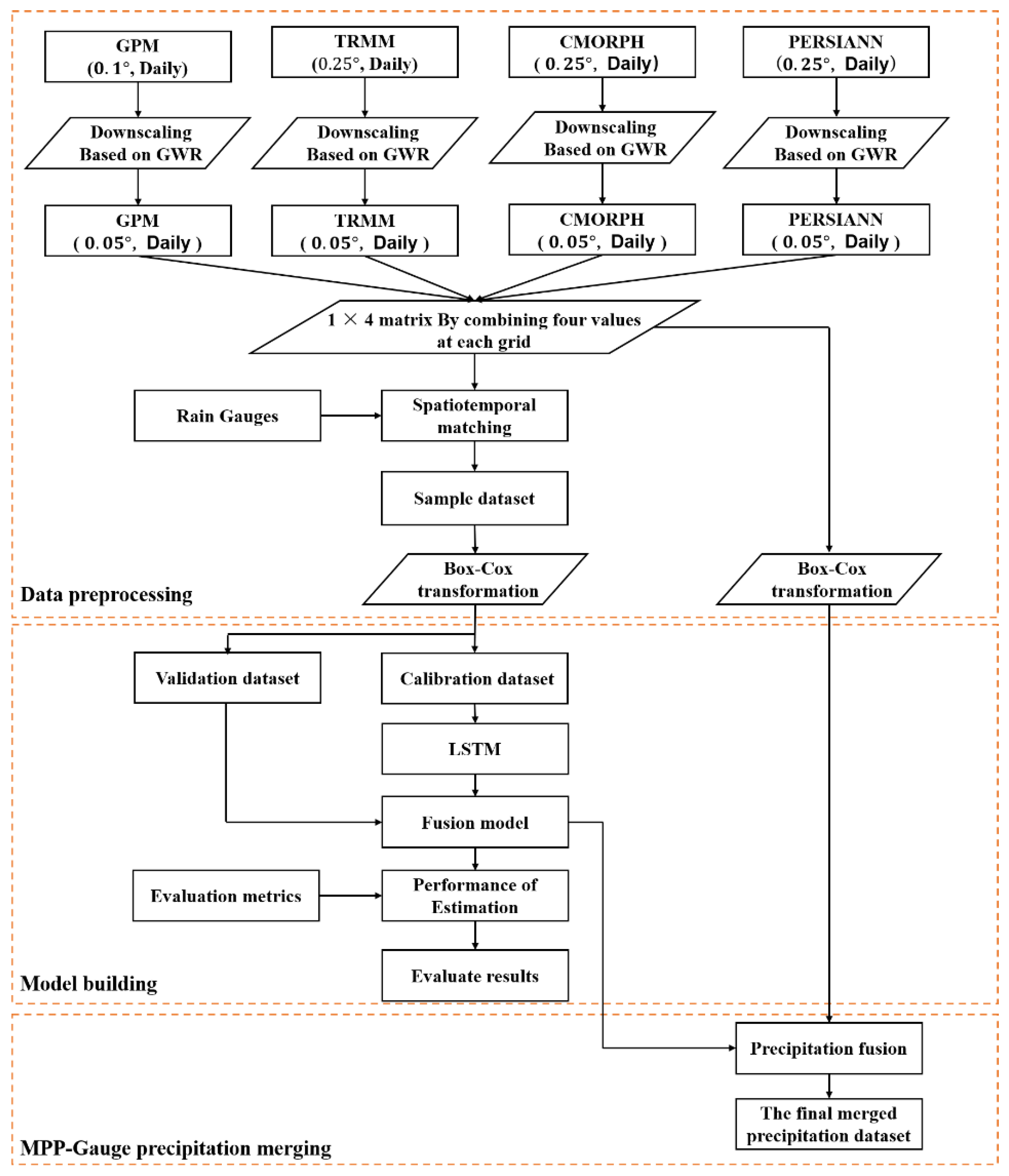
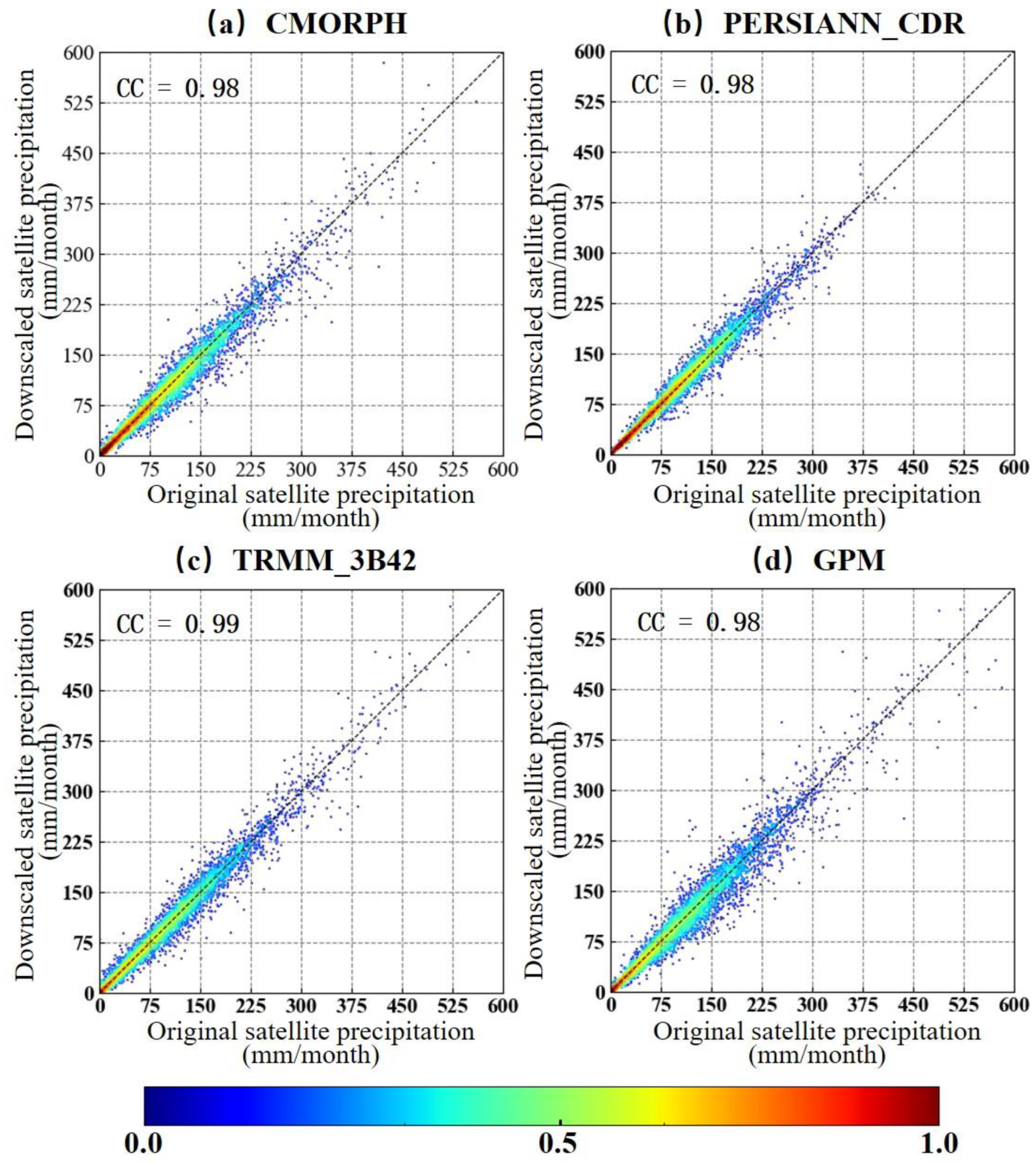
To generate high-resolution spatial precipitation estimations, the original SPPs (GMP, TRMM, CMORPH, and PERSIANN-CDR) are downscaled to 0.05° based on the constructed relationship between precipitation and explanatory variables (NVDI, elevation, slope, longitude, latitude) by the GWR model. The relationship at the original low resolution can be used to predict precipitation with the explanatory variables at a high resolution. Due to the fact that relationship at a daily scale is far less statistically significant than that at monthly scales [37], this study constructs the relationship between precipitation and explanatory variables at a monthly scale by the GWR model, and then disaggregates the downscaled monthly result into daily precipitation to generate the downscaled daily SPP. The specific steps are shown as follows:
Step (1): Resample the explanatory variables (NVDI, elevation, slope, longitude, latitude) from 0.05 ° resolution to 0.25 ° and 0.1 ° resolutions using a bilinear interpolation. The monthly NVDI of 0.05 ° resolution is marked as NVDI m 0.05 , and the resampled NVDIs are marked as NVDI m 0.25 and NVDI m 0.1 , respectively. The 0.05 ° resolution elevation, slope, longitude, and latitude data are marked as Elevation 0.05 , Slope 0.05 , Lon 0.05 , and Lat 0.05 , respectively, and the resampled 0.1 ° and 0.25 ° resolution elevation, slope, longitude, and latitude data are marked as Elevation 0.1 , Slope 0.1 , Lon 0.1 , Lat 0.1 , Elevation 0.25 , Slope 0.25 , Lon 0.25 , and Lat 0.25 , respectively.
Step (2): Construct the relationship between monthly precipitation (accumulate original satellite daily precipitation) and explanatory variables (the resampled NDVI, elevation, slope, longitude, and latitude) by the GWR. The original 0.25 ° resolution satellite daily precipitation (TRMM, CMORPH, and PERSIANN-CDR) is marked as P d 0.25 , TRMM , P d 0.25 , CMO , and P d 0.25 , PER . The original 0.1 ° resolution satellite daily precipitation (GPM) is marked as P d 0.1 , GPM . The accumulated 0.25 ° resolution satellite monthly precipitation (TRMM, CMORPH, and PERSIANN-CDR) is marked as P m 0.25 , TRMM , P m 0.25 , CMO , and P m 0.25 , PER . The accumulated 0.1 ° resolution satellite monthly precipitation (GPM) is marked as P m 0.1 , GPM . The constructed relationship between the satellite precipitation data P m 0.25 , SAT (representing P m 0.25 , TRMM , P m 0.25 , CMO , and P m 0.25 , PER ) and the explanatory variables ( NVDI m 0.25 , Elevation 0.25 , Slope 0.25 , Lon 0.25 , and Lat 0.25 ) is shown in Equation (4). The constructed relationship between the satellite precipitation P m 0.1 , SAT (representing P m 0.1 , GPM ) and the explanatory variables ( NVDI m 0.1 , Elevation 0.1 , Slope 0.1 , Lon 0.1 , Lat 0.1 ) is shown in Equation (5):
P m 0.25 , SAT = α m 0.25 , SAT , 0 + α m 0.25 , SAT , 1 * NVDI m 0.25 + α m 0.25 , SAT , 2 * Elevation 0.25 + α m 0.25 , SAT , 3 * Slope 0.25 + α m 0.25 , SAT , 4 * Lon 0.25 + α m 0.25 , SAT , 5 * Lat 0.25 + ε m 0.25 , SAT
P m 0.1 , SAT = α m 0.1 , SAT , 0 + α m 0.1 , SAT , 1 * NVDI m 0.1 + α m 0.1 , SAT , 2 * Elevation 0.1 + α m 0.1 , SAT , 3 * Slope 0.1 + α m 0.1 , SAT , 4 * Lon 0.1 + α m 0.1 , SAT , 5 * Lat 0.1 + ε m 0.1 , SAT
where α m 0.25 , SAT , 0 and α m 0.1 , SAT , 0 are the intercepts; α m 0.25 , SAT , 1 , α m 0.25 , SAT , 2 , α m 0.25 , SAT , 3 , α m 0.25 , SAT , 4 , α m 0.25 , SAT , 5 , α m 0.1 , SAT , 1 , α m 0.1 , SAT , 2 , α m 0.1 , SAT , 3 , α m 0.1 , SAT , 4 , and α m 0.1 , SAT , 5 are the regression coefficients; and ε m 0.25 , SAT and ε m 0.1 , SAT are residuals of the two GWR models.
Step (3): Resample the regression coefficients ( α m 0.25 , SAT , 0 , α m 0.25 , SAT , 1 , α m 0.25 , SAT , 2 , α m 0.25 , SAT , 3 , α m 0.25 , SAT , 4 , α m 0.25 , SAT , 5 , α m 0.1 , SAT , 0 , α m 0.1 , SAT , 2 , α m 0.1 , SAT , 3 , α m 0.1 , SAT , 4 , and α m 0.1 , SAT , 5 ) to obtain the 0.05 ° resolution regression coefficients ( α m 0.05 0 , SAT , 0 , α m 0.05 0 , SAT , 1 , α m 0.05 0 , SAT , 2 , α m 0.05 0 , SAT , 3 , α m 0.05 0 , SAT , 4 , and α m 0.05 0 , SAT , 5 ) by the bilinear interpolation method, and resample the residuals ( ε m 0.25 , SAT , ε m 0.1 , SAT ) to obtain the 0.05 ° resolution residuals ( ε m 0.05 , SAT ) by the ordinary kriging interpolation method.
Step (4): Estimate monthly precipitation ( P m 0.05 , SAT ) by using the resampled 0.05 ° resolution regression coefficients ( α m 0.05 0 , SAT , 0 , α m 0.05 0 , SAT , 1 , α m 0.05 0 , SAT , 2 , α m 0.05 0 , SAT , 3 , α m 0.05 0 , SAT , 4 , and α m 0.05 0 , SAT , 5 ), and the resampled 0.05 ° resolution residuals ( ε m 0.25 , SAT , ε m 0.1 , SAT ) are shown in Equation (6).
P m 0.05 , SAT = α m 0.05 , SAT , 0 + α m 0.05 , SAT , 1 * NVDI m 0.05 + α m 0.05 , SAT , 2 * Elevation 0.05 + α m 0.05 , SAT , 3 * Slope 0.05 + α m 0.05 , SAT , 4 * Lon 0.05 + α m 0.05 , SAT , 5 * Lat 0.05 + ε m 0.05 , SAT
Step (5): Disaggregate the downscaled satellite monthly precipitation into daily precipitation according to a proportional fraction. The fraction of the 0.25 ° and 0.1 ° resolution daily precipitation to the 0.25 ° and 0.1 ° resolution monthly precipitation is denoted as F d 0.25 , SAT and F d 0.1 , SAT , respectively. F d 0.25 , SAT and F d 0.1 , SAT are calculated by Equation (7).
F d 0.25 , SAT = P d 0.25 , SAT P m 0.25 , SAT , F d 0.1 , SAT = P d 0.1 , SAT P m 0.1 , SAT
Next, the 0.25 ° and 0.1 ° resolution fractions ( F d 0.25 , SAT and F d 0.1 , SAT ) are resampled to obtain the 0.05 ° resolution fraction ( F d 0.05 , SAT ) by a bilinear interpolation method. Then, Equation (8) is used to obtain the 0.05 ° resolution daily precipitation.
P d 0.05 , SAT = F d 0.05 , SAT * P m 0.05 , SAT
P d 0.05 , SAT represents the 0.05 ° resolution daily precipitation (the downscaled TRMM, CMORPH, PERSIANN-CDR, and GPM).

2.2.2. Calibration and Validation Dataset Generation

As shown in Figure 3, for each grid, 1 × 4 matrix data centered on it are extracted day by day from the downscaled SPPs (TRMM, CMORPH, PERSIANN-CDR, and GMP). Then, the extracted matrix data are matched with the daily time series of rain gauges in chronological order and geographic coordinates to generate a sample dataset. Due to the spatiotemporal intermittency of daily precipitation, the generated dataset from the original SPPs contains a large number of zero values (no rain). Directly using the generated dataset to train the deep neural network will lead to the failure of training work. To solve this issue, Box–Cox transformation [38,39] was used to transform the generated dataset to a new sample dataset. The Box–Cox transformation, also called the power transformation, transforms a non-normally distributed variable to a normally distribute one [40]. The Box–Cox transformation is shown as in Equation (9):
P i T = ( P i S A T ) δ 1 δ
where P i T is the precipitation value after Box–Cox transformation at location i , and P i SAT is the precipitation value at location i before Box–Cox transformation. The optimal value of δ changes slightly with the number of days, 87% of which is between 0.2 and 0.3, and the annual average is close to 0.25 [39]. In this study, a fixed value of 0.25 is used.
Finally, the calibration dataset and the validation dataset are generated according to a certain proportion.

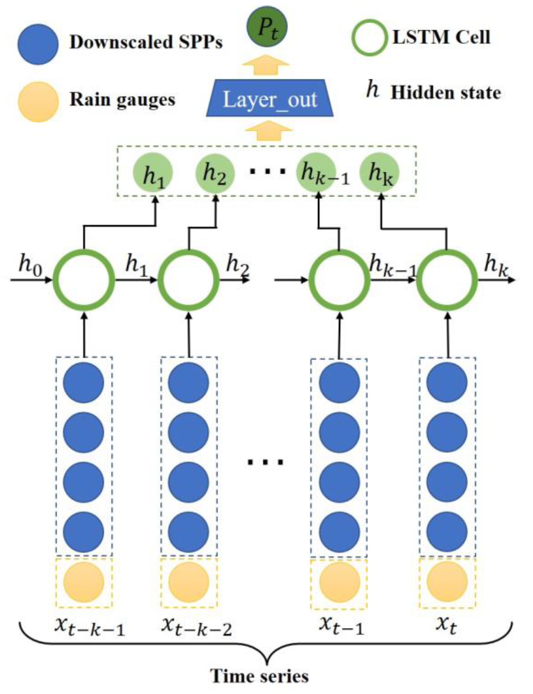
2.2.3. Fusion by LSTM Network

A long short-term memory (LSTM) network, which is composed of an input layer, one or more memory cells, and an output layer, is well suited to study time series data [41]. The main structure of an LSTM network contains so-called memory cell in the hidden layer. The memory cell controls the communication of information within the memory cells through three gates (i.e., input gate i t , forget gate f t , and output gate o t ). Each gate controls the information to participate in the update of the memory state and selectively retains or discards information. The key equation of the LSTM network is shown as follows:
i t = σ ( w x i x t + w h i h t 1 + w c i c t 1 + b i ) f t = σ ( w x f x t + w h f h t 1 + w c f c t 1 + b f ) c t = f t c t 1 + i t tanh ( w x c x t + w h c h t 1 + b c ) o t = σ ( w x o x t + w h o h t 1 + w c o c t 1 + b o ) h t = o t tanh ( c t )
where “ ” represents element-wise multiplication, x t represents the input vector at time t, each w represents the adjustable weight of the network, b represents the adjustable bias vector, h represents the internal hidden state, c represents the cell state of the memory cell, and σ represents the activation function.
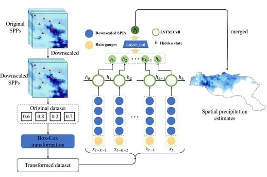
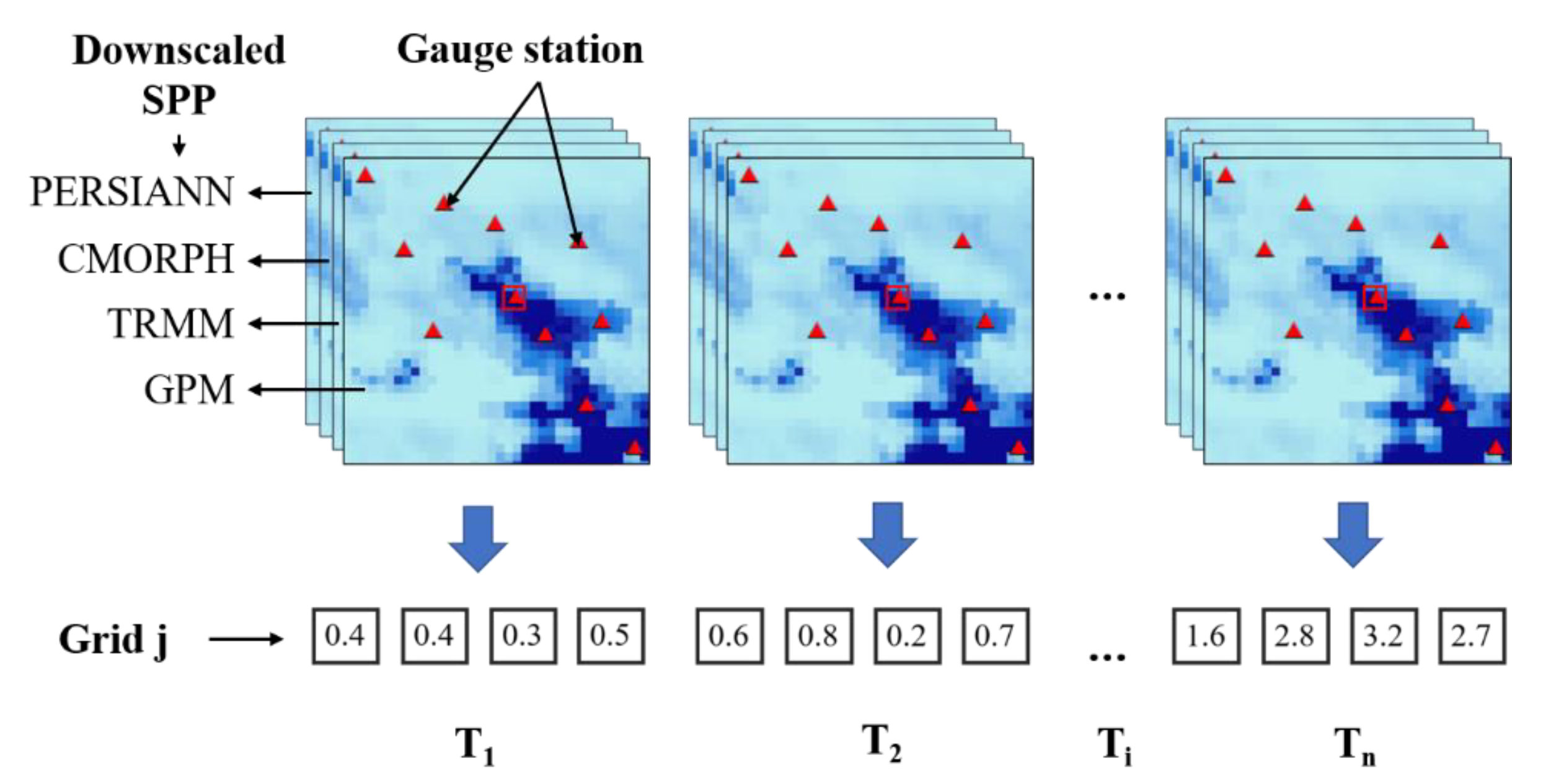
As shown in 
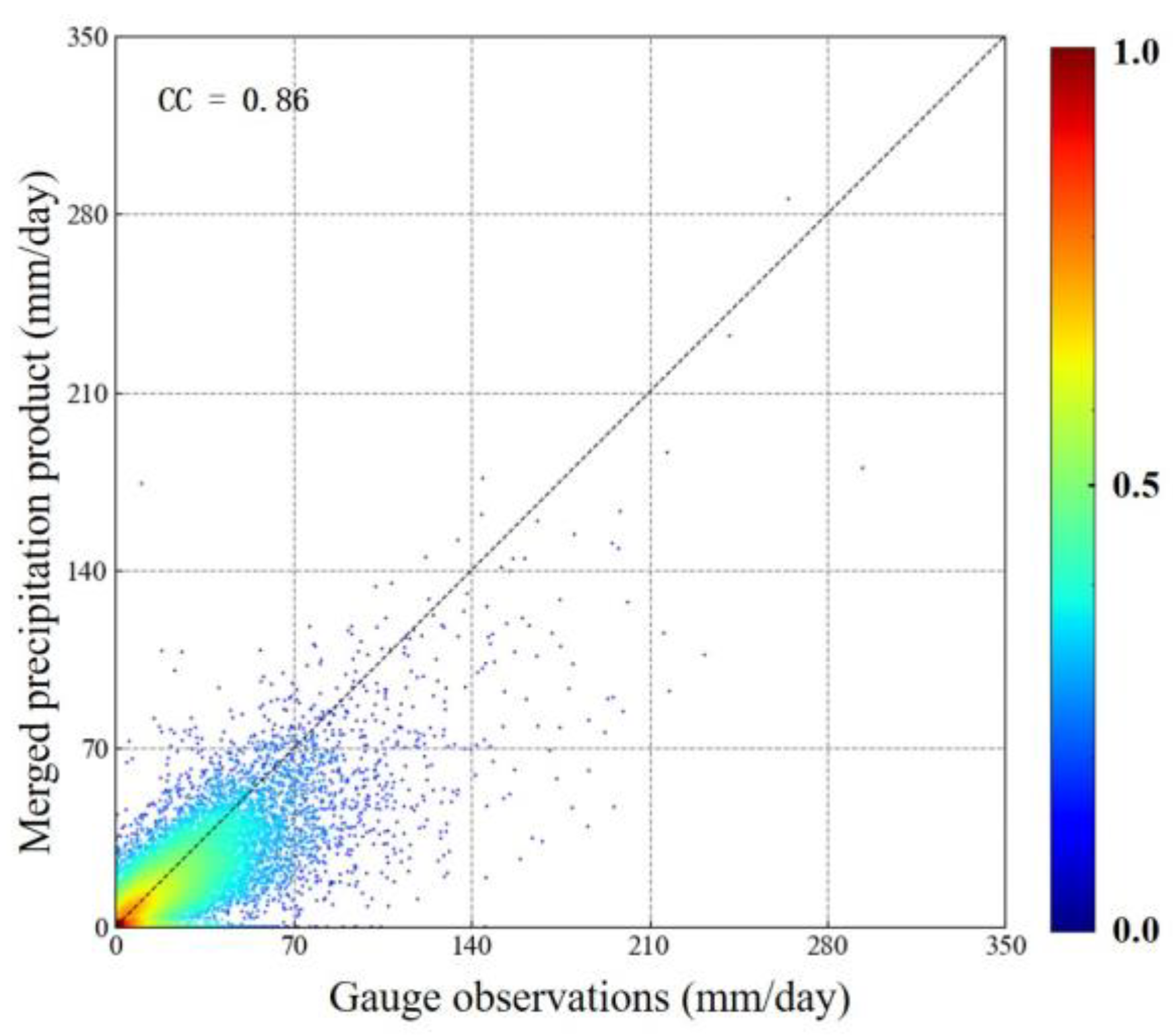
Figure 4, this study uses the LSTM network for improving the estimation accuracy of spatial precipitation by exploiting the spatiotemporal correlation pattern between multisatellite precipitation products and rain gauges. The LSTM network extracts the spatiotemporal correlation patterns through a series of memory cells and merges those extracted patterns to generate high-quality daily precipitation estimates. The key to the LSTM-based fusion to realize long-term memory lies in keeping the multiple precipitation information of each time step in the memory cells. For a certain time step, the multiple precipitation information at the past moment will be retained in the memory cells, and provide a reference for the merged precipitation at the current moment. In this fusion model, the LSTM network includes multiple memory cells in the hidden layers. The output neurons (the extracted spatiotemporal patterns of multisatellite precipitation) at the last time step from the last hidden layer of the LSTM network are merged to a single output neuron (the merged precipitation) through the fully connected network.
In this paper, we trained the LSTM network with four SPPs (TRMM, CMORPH, PERSIANN-CDR, and GMP) as input and gauge observations as output. The specific hyperparameters (i.e., number of layers, number of neurons, learning rate, and epoch) of this fusion model were the optimal choices based on the data size and multiple experiments. The epoch and learning rate of the LSTM network were 200 and 0.01, respectively. The number of hidden layers was 3. The number of neurons in each hidden layer were 128, 128, and 64, respectively.

2.2.4. Evaluation Metrics

A set of evaluation metrics, including the correlation coefficient (CC), root mean square error (RMSE), mean absolute error (MAE), Kling–Gupta efficiency (KGE), probability of detection (POD), false alarm ratio (FAR), bias rate (BIAS), and equity threatened score (ETS), is selected to evaluate the results of the GWRR-LSTM framework. The evaluation metrics used in this study are listed in Table 2. CC reflects the degree of linear correlation between the estimations and observations, RMSE reflects the overall error level and fluctuation of the estimations, MAE represents the average absolute deviation between the estimations and the observations, and the KGE coefficient considers different types of model errors (the error in the mean, the variability, and the dynamics). Four categorical metrics (POD, FAR, BIAS, and ETS) are selected to evaluate the ability of the GWRR-LSTM framework to identify whether precipitation occurs and to capture precipitation events of different intensities (0.1, 10, 25, and 50 mm/d). The probability of detection POD represents the probability that actual precipitation is correctly detected, the false alarm rate FAR represents the probability of errors, the BIAS reflects whether precipitation is overestimated or underestimated, and the ETS reflects the comprehensive detection accuracy of the estimations in different times and spaces.

3. Results

The integrated framework (GWR-LSTM) was applied to estimate daily spatial precipitation from the data of rain gauges and four SPPs (TRMM_3B42, CMORPH, PERSIANN-CDR, and GPM) in the Hanjiang River Basin of China during the period of 2007–2018. The application effect was evaluated and analyzed.

3.1. Merged Precipitation Product (MPP)

Figure 5 shows the scatter density plots between the downscaled monthly precipitation (0.05°) based on the GWR model and the original satellite monthly precipitation (0.25° for TRMM_3B42, CMORPH, and PERSIANN and 0.1° for GPM) during the period of 2007 to 2018. The CC values are 0.98, 0.98, 0.99, and 0.98. The GWR for downscaling performed well for all original four SPPs. In addition, Figure 5 verifies the conclusion of Chen et al. [18] that the vegetation index (NVDI), elevation, slope, and geographical location have a very stable relationship with the four SPPs at a monthly scale for different spatial resolutions, which benefits the spatial downscaling.
Figure 6 shows the scatter density plots between gauge observations and the final merged precipitation product (MPP) generated by the GWR-LSTM framework, with a CC of 0.86, which indicates that the GWR-LSTM framework performed well for merging multisatellite precipitation products and gauge precipitation. Figure 7 shows the spatial daily precipitation estimates from the gauge observations, the final MPP, the original four daily SPPs, and the downscaled daily SPPs on 9 August 2007. The MPP and the downscaled daily SPPs provide more detailed information, but their spatial patterns are different. The spatial pattern of the original GPM is similar to the original PERSIANN-CDR and TRMM_3B42 and significantly different from the gauge observations. The spatial patterns of the original CMORPH and the MPP are similar to the gauge observations, but the spatial pattern of MPP is more consistent with that of the gauge observations. In addition, the maximum daily precipitation of CMORPH is 20.49 mm/day, which is far lower than the maximum daily precipitation of the gauge observations (103.8 mm/day). In summary, the MPP has more accurate and detailed spatial representativeness than any other original or downscaled SPPs.
Table 3 shows the performances for the original SPPs, the downscaled SPPs, and the final MPP with reference to gauge observations during 2007–2018. There is little difference between the performances of the original four SPPs and the downscaled four SPPs. Therefore, the above results lead to the preliminary conclusion that the GWR model only downscales for the original SPPs without improving the SPPs’ accuracy, and the accuracy improvement of spatial precipitation estimates is owing to the powerful feature extraction ability of the LSTM network.

3.2. Performance Evaluation of MPP

Figure 8 shows the time series of average monthly precipitation of original SPPs and MPP, gauge observations at the whole basin from 2007 to 2018. The time series of original SPPs and MPP are similar to the gauge observations, but the time series of MPP is more consistent with that of gauge observations. Table 4 shows the evaluation results of four continuity metrics (CC, MAE, RMSE, and KGE) of the original four SPPs (TRMM, PERSIANN, CMORPH, and GPM) and the final MPP across the entire period and different seasons from 2007 to 2018. All these indices of MPP had much better scores than the four original SPPs, indicating that the GWR-LSTM framework substantially improved the accuracy of the daily precipitation estimates. The continuous indices of MPP had the best scores in autumn, followed by spring, summer, and winter. However, due to the winter snowfall, the original four SPPs cannot capture the spatial pattern of precipitation well, and the MPP derived from the original four SPPs did not perform perfectly in winter.
Table 5 shows the evaluation results of four continuity metrics (CC, MAE, RMSE, and KGE) of the original four SPPs (TRMM, PERSIANN, CMORPH, and GPM) and the final MPP at the upper, middle, and lower reaches of the Hanjiang River during 2007–2018. There are differences among metrics of the original four SPPs. Each SPP has its own advantages and disadvantages in capturing the spatiotemporal pattern of precipitation in different regions. All CMORPH metrics are better than those of the other three SPPs (TRMM, PERSIANN, and GPM). Metrics of PERSIANN performed worst in the upper, middle, and lower reaches of the Hanjiang River and the whole basin. All metrics of MPP performed better than the original four SPPs, CC was increased by approximately 56%, MAE was decreased by approximately 49%, RMSE was decreased by approximately 39%, and KGE was increased by approximately 19%, indicating that the GWR-LSTM framework significantly improves the quality of spatial daily precipitation estimation. The CC exceeded 0.84 at the upper reaches of the Hanjiang River with complex terrain, and the CC reached 0.9 at the lower reaches with a sparse rain gauge network, indicating that the GWR-LSTM framework proposed in this paper has good adaptability.
Figure 9 visually compares the estimation accuracy of daily precipitation from the final MPP, the original four SPPs, and the gauge observation through a Taylor diagram. The point of MPP was closer to the gauge point than any other original four SPPs at the upper, middle, and lower reaches and the whole Hanjiang River Basin. Figure 9 also confirms that the fusion model based on the GWR-LSTM framework significantly improves the estimation accuracy of daily spatial precipitation, especially in the lower reaches with flat terrain.
Figure 10 shows the statistical results of the four categorical metrics (POD, FAR, BIAS, and ETS) for four types of precipitation intensity (0.1, 10, 25, and 50 mm/d). As shown in Figure 10a, the final MPP and original four SPPs identify the no rain events well, but MPP shows better performance than the original four SPPs in rainy event detection. As shown in Figure 10b, with the increase in precipitation intensity, the FAR of all the products also increased, but the FAR of MPP was significantly lower than that of any other SPP under different precipitation intensities. As shown in Figure 10c, the MPP underestimated the amount of all rain events, and the other four SPPs obviously overestimated the number of no-rain events and underestimated the amount of light rain, moderate rain, or heavy rain events. As shown in Figure 10d, the comprehensive detection accuracy of MPP was significantly higher than that of the other four SPPs. In terms of the four categorical metrics, the GWR-LSTM framework significantly improved the estimation accuracy of the daily spatial precipitation.

3.3. Comparisons

3.3.1. Comparison with Other Fusion Models

Table 6 shows the evaluation results of the GWR-LSTM framework, the simple model average method (SMA) [42], and the geographically weighted ridge regression method (GWRR) [18] across the whole, upper, middle, and lower reaches of the Hanjiang River from 2007 to 2018. The GWR-LSTM framework obtained much better scores than the other two fusion models (SMA, GWRR) on these metrics for the whole Hanjiang River Basin, indicating that the GWR-LSTM framework well improved the estimation accuracy of the daily precipitation. The SMA model performed the worst. The GWRR framework performed excellently, but at the lower reaches of the Hanjiang River Basin with a sparse rain gauge network, all the evaluation metrics of GWRR were relatively poor. Figure 11 shows the spatial distribution of the MAE for the estimated daily precipitation by the three models (GWR-LSTM, GWRR, SMA). The MAE value of the SMA model is large over the whole Hanjiang River Basin; the MAE value of the GWRR model was large only in the lower reaches of the Hanjiang River Basin, which has a sparse rain gauge network density, while the MAE of the GWR-LSTM framework is evenly distributed over the whole basin. The GWR-LSTM framework significantly improves the estimation of spatial daily precipitation, especially in areas with sparse rain gauge networks.

3.3.2. Comparison with Different Combinations of SPPs

An important factor, which affects the performance of the fusion model, is the abilities of SPPs to capture the spatiotemporal patterns of precipitation [15,18]. Because no SPP is superior to other products at all times and regions [25], it is necessary to evaluate the performance of various SPPs for merging. Table 7 shows the evaluation results of the spatial precipitation estimates generated by the GWR-LSTM framework merging different combinations of SPPs and gauge precipitations. ModelTC represents the fusion model for merging TRMM, CMORPH, and gauge precipitation; ModelTP represents the fusion model for merging TRMM, PERSIANN, and gauge precipitation; ModelTG represents the fusion model for merging TRMM, GPM, and gauge precipitation; ModelCP represents the fusion model for merging CMORPH, PERSIANN, and gauge precipitation; ModelCG represents the fusion model for merging CMORPH, GPM, and gauge precipitation; ModelPG represents the fusion model for merging PERSIANN, GPM, and gauge precipitation; ModelTCP represents the fusion model for merging TRMM, CMORPH, PERSIANN, and gauge precipitation; ModelTCG represents the fusion model for merging TRMM, CMORPH, GPM, and gauge precipitation; ModelCPG represents the fusion model for merging CMORPH, PERSIANN, GPM, and gauge precipitation; ModelTCPG represents the fusion model for merging TRMM, CMORPH, PERSIANN, GPM, and gauge precipitation. As listed in Table 7, the results of all combinations of SPPs have significantly improved the accuracy of spatial precipitation estimates, but the results of four SPPs in this paper are the best. In this study, the use of multisatellite precipitation products can make full use of the advantages of each SPP, without selecting a well-performing SPP or multiple well-performing SPPs for merging.

4. Discussion

To investigate whether a multi-SPP fusion model performs well compared with a single-SPP fusion model, we compared a fusion model for merging a single-satellite and gauge precipitation. Unlike the fusion model for merging multisatellite and gauge precipitation, the fusion model for merging a single-satellite and gauge precipitation generally introduces relevant auxiliary factors, such as elevation and brightness temperature. Wu et al. [4] proposed a CNN-LSTM fusion model for merging single-satellite and gauge precipitation. In this paper, we used the CNN-LSTM model and relevant auxiliary factors (elevation and brightness temperature) to merge four SPPs (TRMM_3B42, CMORPH, PERSIANN-CDR, and GPM) and gauge precipitation. The constructed models were marked as ModelT, ModelC, ModelP, and ModelG. Figure 12 visually compares the performance of the four models (ModelT, ModelC, ModelP, and ModelG) and the GWR-LSTM framework through a Taylor diagram. The four fusion models, which used different single-satellite precipitation products, can improve the accuracy of spatial precipitation estimation. Due to the different abilities of SPP capturing the spatial pattern of precipitation, the four fusion models (ModelT, ModelC, ModelP, and ModelG) have different accuracies of spatial precipitation estimation. The CC values of spatial precipitation estimated by the four fusion models (ModelT, ModelC, ModelP, and ModelG) were 0.62, 0.59, 0.68, and 0.60, respectively. The evaluation results (CC was 0.86, MAE was 1.26, RMSE was 4.55, and KGE was 0.60) of spatial precipitation estimated by the GWR-LSTM framework can fully show that using multiple SPPs can provide more reliable spatial precipitation estimation than using a single SPP, which is consistent with the conclusion of Chen et al. [18].
There are still some limitations and uncertainties in the study. The spatial scale mismatch between the SPPs and gauge observations was neglected. The neglect would affect the satellite–gauge merging results and, meanwhile, bring some biases to the performance assessments of the precipitation products, especially over the regions of complex topography [19]. Although downscaling for the SPPs might help to ameliorate the influences of the spatial scale mismatch, the mismatch may still exist. In addition, this study first downscales for the SPPs based on GWR using explanatory variables (NVDI, elevation, slope, longitude, and latitude). The GWR may be highly susceptible to a collinearity problem [43]. We should first diagnose whether collinearity exists, and then solve this problem in future.

5. Conclusions

In this paper, an integrated framework for merging multisatellite and gauge precipitation was proposed. The framework integrates the geographically weighted regression (GWR) for improving the spatial resolution of precipitation estimations and the long short-term memory (LSTM) network for improving the precipitation estimation accuracy by exploiting the spatiotemporal correlation pattern between multisatellite precipitation products and rain gauges. The GWR-LSTM framework was applied to estimate the daily spatial precipitation in the Hanjiang River Basin of China from 2007 to 2018. The main findings of this study are as follows:
(1)
The proposed framework (GWR-LSTM) can significantly improve the spatial resolution and accuracy of precipitation estimates (resolution of 0.05°, CC of 0.86, and KGE of 0.6) over original SPPs (resolution of 0.25 ° or 0.1 ° , CC of 0.36–0.54, KGE of 0.30–0.52), and this study also demonstrates that the use of merging multiple-satellite and gauges precipitation is much better than merging partial datasets of multiple-satellite precipitation with gauge observations (Table 7).
(2)
In the fusion process, the GWR model only downscales for the original SPPs without improving the SPP accuracy, and the accuracy improvement of spatial precipitation estimates is owing to the powerful feature extraction ability of the LSTM network.
In summary, the proposed framework (GWR-LSTM) can be applied to merge multisatellite and gauge precipitation, which improves daily spatial precipitation estimations. Multisource precipitation observation data represented by ground rain gauges, weather radar, and space satellites are descriptions of precipitation information in different modes facing the same observation object. In the future work, multisource precipitation observation data and multimodal deep learning data fusion methods can be combined to fully exploit the advantages of each satellite product data and further improve the accuracy of spatial precipitation estimation.

Author Contributions

Methodology, conceptualization, formal analysis, and writing—original draft, J.S.; methodology and writing—review and editing, P.L.; investigation, Y.D. and Y.Z; data analysis, P.L., J.S. and Y.Z.; funding acquisition and resources, J.X. All authors have read and agreed to the published version of the manuscript.

Funding

This study was supported by the Strategic Priority Research Program of the Chinese Academy of Sciences (Grant No. XDA23040304) and the National Natural Science Foundation of China (41890823).

Acknowledgments

We thank the anonymous reviewers for their constructive feedback.

Conflicts of Interest

The authors declare no conflict of interest.

References

  1. Xu, Q.; Chen, J.; Peart, M.R.; Ng, C.N.; Hau, B.C.H.; Law, W.W.Y. Exploration of severities of rainfall and runoff extremes in ungauged catchments: A case study of Lai Chi Wo in Hong Kong, China. Sci. Total Environ. 2018, 634, 640–649. [Google Scholar] [CrossRef] [PubMed]
  2. Yang, K.; Wu, H.; Qin, J.; Lin, C.; Tang, W.; Chen, Y.J.G.; Change, P. Recent climate changes over the Tibetan Plateau and their impacts on energy and water cycle: A review. Glob. Planet. Chang. 2014, 112, 79–91. [Google Scholar] [CrossRef]
  3. Brodeur, Z.P.; Steinschneider, S. Spatial Bias in Medium-Range Forecasts of Heavy Precipitation in the Sacramento River Basin: Implications for Water Management. J. Hydrometeorol. 2020, 21, 1405–1423. [Google Scholar] [CrossRef]
  4. Wu, H.; Yang, Q.; Liu, J.; Wang, G. A spatiotemporal deep fusion model for merging satellite and gauge precipitation in China. J. Hydrol. 2020, 584, 124664. [Google Scholar] [CrossRef]
  5. Verdin, A.; Rajagopalan, B.; Kleiber, W.; Funk, C. A Bayesian kriging approach for blending satellite and ground precipitation observations. Water Resour. Res. 2015, 51, 908–921. [Google Scholar] [CrossRef]
  6. Lu, D.; Yong, B. Evaluation and Hydrological Utility of the Latest GPM IMERG V5 and GSMaP V7 Precipitation Products over the Tibetan Plateau. Remote Sens. 2018, 10, 2022. [Google Scholar] [CrossRef]
  7. Xiao, S.; Zou, L.; Xia, J.; Yang, Z.; Yao, T. Bias correction framework for satellite precipitation products using a rain/no rain discriminative model. Sci. Total Environ. 2022, 818, 151679. [Google Scholar] [CrossRef]
  8. Bharti, V.; Singh, C. Evaluation of error in TRMM 3B42V7 precipitation estimates over the Himalayan region. J. Geophys. Res. Atmos. 2015, 120, 12458–12473. [Google Scholar] [CrossRef]
  9. Todini, E. A Bayesian technique for conditioning radar precipitation estimates to rain-gauge measurements. Hydrol. Earth Syst. Sci. 2001, 5, 187–199. [Google Scholar] [CrossRef]
  10. Seo, D.-J.; Breidenbach, J.P. Real-Time Correction of Spatially Nonuniform Bias in Radar Rainfall Data Using Rain Gauge Measurements. J. Hydrometeorol. 2001, 3, 93–111. [Google Scholar] [CrossRef]
  11. Thorndahl, S.; Nielsen, J.E.; Rasmussen, M.R. Bias adjustment and advection interpolation of long-term high resolution radar rainfall series. J. Hydrol. 2014, 508, 214–226. [Google Scholar] [CrossRef]
  12. Shen, Y.; Zhao, P.; Pan, Y.; Yu, J. A high spatiotemporal gauge-satellite merged precipitation analysis over China. J. Geophys. Res. Atmos. 2014, 119, 3063–3075. [Google Scholar] [CrossRef]
  13. Yan, J.; Bárdossy, A. Short time precipitation estimation using weather radar and surface observations: With rainfall displacement information integrated in a stochastic manner. J. Hydrol. 2019, 574, 672–682. [Google Scholar] [CrossRef]
  14. Beck, H.E.; van Dijk, A.I.J.M.; Levizzani, V.; Schellekens, J.; Miralles, D.G.; Martens, B.; de Roo, A. MSWEP: 3-hourly 0.25° global gridded precipitation (1979–2015) by merging gauge, satellite, and reanalysis data. Hydrol. Earth Syst. Sci. 2017, 21, 589–615. [Google Scholar] [CrossRef]
  15. Chao, L.; Zhang, K.; Li, Z.; Zhu, Y.; Wang, J.; Yu, Z. Geographically weighted regression based methods for merging satellite and gauge precipitation. J. Hydrol. 2018, 558, 275–289. [Google Scholar] [CrossRef]
  16. Miao, Q.; Pan, B.; Wang, H.; Hsu, K.; Sorooshian, S. Improving Monsoon Precipitation Prediction Using Combined Convolutional and Long Short Term Memory Neural Network. Water 2019, 11, 977. [Google Scholar] [CrossRef]
  17. Kumar, A.; Ramsankaran, R.; Brocca, L.; Munoz-Arriola, F. A Machine Learning Approach for Improving Near-Real-Time Satellite-Based Rainfall Estimates by Integrating Soil Moisture. Remote Sens. 2019, 11, 2221. [Google Scholar] [CrossRef]
  18. Chen, S.; Xiong, L.; Ma, Q.; Kim, J.-S.; Chen, J.; Xu, C.-Y. Improving daily spatial precipitation estimates by merging gauge observation with multiple satellite-based precipitation products based on the geographically weighted ridge regression method. J. Hydrol. 2020, 589, 125156. [Google Scholar] [CrossRef]
  19. Zhang, L.; Li, X.; Zheng, D.; Zhang, K.; Ge, Y. Merging multiple satellite-based precipitation products and gauge observations using a novel double machine learning approach. J. Hydrol. 2021, 594, 125969. [Google Scholar] [CrossRef]
  20. Huffman, G.J.; Adler, R.F.; Arkin, P.; Chang, A.; Ferraro, R.; Gruber, A.; Janowiak, J.; McNab, A.; Rudolf, B.; Schneider, U. The Global Precipitation Climatology Project (GPCP) Combined Precipitation Dataset. Bull. Am. Meteorol. Soc. 1997, 78, 5–20. [Google Scholar] [CrossRef]
  21. Kummerow, C.; Simpson, J.; Thiele, O.; Barnes, W.; Chang, A.; Stocker, E.; Adler, R.F.; Hou, A.; Kakar, R.; Wentz, F.; et al. The Status of the Tropical Rainfall Measuring Mission (TRMM) after Two Years in Orbit. J. Appl. Meteorol. 2000, 39, 1965–1982. [Google Scholar] [CrossRef]
  22. Joyce, R.J.; Janowiak, J.E.; Arkin, P.A.; Xie, P. CMORPH: A Method that Produces Global Precipitation Estimates from Passive Microwave and Infrared Data at High Spatial and Temporal Resolution. J. Hydrometeorol. 2004, 5, 287–296. [Google Scholar] [CrossRef]
  23. Hong, Y.; Hsu, K.L.; Sorooshian, S.; Gao, X. Precipitation Estimation from Remotely Sensed Imagery using an Artificial Neural Network Cloud Classification System. J. Appl. Meteorol. 2004, 36, 1176–1190. [Google Scholar] [CrossRef]
  24. Kubota, T.; Shige, S.; Hashizume, H.; Aonashi, K.; Takahashi, N.; Seto, S.; Hirose, M.; Takayabu, Y.N.; Ushio, T.; Nakagawa, K.; et al. Global Precipitation Map Using Satellite-Borne Microwave Radiometers by the GSMaP Project: Production and Validation. IEEE Trans. Geosci. Remote Sens. 2007, 45, 2259–2275. [Google Scholar] [CrossRef]
  25. Sun, Q.; Miao, C.; Duan, Q.; Ashouri, H.; Sorooshian, S.; Hsu, K.L. A Review of Global Precipitation Data Sets: Data Sources, Estimation, and Intercomparisons. Rev. Geophys. 2018, 56, 79–107. [Google Scholar] [CrossRef]
  26. Rahman, K.U.; Shang, S.; Shahid, M.; Wen, Y.; Khan, Z. Application of a Dynamic Clustered Bayesian Model Averaging (DCBA) Algorithm for Merging Multisatellite Precipitation Products over Pakistan. J. Hydrometeorol. 2020, 21, 17–37. [Google Scholar] [CrossRef]
  27. Rahman, K.; Shang, S.; Shahid, M.; Li, J. Developing an Ensemble Precipitation Algorithm from Satellite Products and Its Topographical and Seasonal Evaluations Over Pakistan. Remote Sens. 2018, 10, 1835. [Google Scholar] [CrossRef]
  28. Ma, Y.; Yang, H.; Yang, C.; Yuan, Y.; Tang, G.; Yao, Y.; Di, L.; Li, C.; Han, Z.; Liu, R. Performance of Optimally Merged Multisatellite Precipitation Products Using the Dynamic Bayesian Model Averaging Scheme Over the Tibetan Plateau. J. Geophys. Res. Atmos. 2018, 123, 814–834. [Google Scholar] [CrossRef]
  29. Chen, H.; Hu, N.; Cheng, Z.; Zhang, L.; Zhang, Y. A deep convolutional neural network based fusion method of two-direction vibration signal data for health state identification of planetary gearboxes. Measurement 2019, 146, 268–278. [Google Scholar] [CrossRef]
  30. Zhang, L.; Xie, Y.; Luan, X.; Xin, Z. Multi-source heterogeneous data fusion. In Proceedings of the 2018 International Conference on Artificial Intelligence and Big Data (ICAIBD), Chengdu, China, 26–28 May 2018. [Google Scholar]
  31. Yu, Y.; Si, X.; Hu, C.; Zhang, J. A Review of Recurrent Neural Networks: LSTM Cells and Network Architectures. Neural Comput. 2019, 31, 1235–1270. [Google Scholar] [CrossRef]
  32. Zhai, J.; Dong, G.; Chen, F.; Xie, X.; Qi, C.; Li, L. A Deep Learning Fusion Recognition Method Based On SAR Image Data. Procedia Comput. Sci. 2019, 147, 533–541. [Google Scholar]
  33. Saleh, K.; Hossny, M.; Nahavandi, S. Driving behavior classification based on sensor data fusion using LSTM recurrent neural networks. In Proceedings of 2017 IEEE 20th International Conference on Intelligent Transportation Systems (ITSC), Yokohama, Japan, 16–19 October 2017. [Google Scholar]
  34. Yang, F.; Zhu, J.; Wang, X.; Wu, X.; Tang, Y.; Luo, L. A Multi-model Fusion Framework based on Deep Learning for Sentiment Classification. In Proceedings of the 2018 IEEE 22nd International Conference on Computer Supported Cooperative Work in Design ((CSCWD)), Nanjing, China, 9–11 May 2018; pp. 433–437. [Google Scholar]
  35. Liu, P.; Zhang, Y.; Bao, F.; Yao, X.; Zhang, C. Multi-type data fusion framework based on deep reinforcement learning for algorithmic trading. Appl. Intell. 2022. [Google Scholar] [CrossRef]
  36. Brunsdon, C.; Fotheringham, A.S.; Charlton, M.E. Geographically Weighted Regression: A Method for Exploring Spatial Nonstationarity. Geogr. Anal. 2010, 28, 281–298. [Google Scholar] [CrossRef]
  37. Chen, F.; Gao, Y.; Wang, Y.; Qin, F.; Li, X. Downscaling satellite-derived daily precipitation products with an integrated framework. Int. J. Climatol. 2019, 39, 1287–1304. [Google Scholar] [CrossRef]
  38. Box, G.; Cox, D. An analysis of transformations. J. Roy. Stat. Soc. 1964, 26A, 211–252. [Google Scholar] [CrossRef]
  39. Erdin, R.; Frei, C.; Kunsch, H.R. Data Transformation and Uncertainty in Geostatistical Combination of Radar and Rain Gauges. J. Hydrometeorol. 2012, 13, 1332–1346. [Google Scholar] [CrossRef]
  40. Kim, M.; Hill, R.C. The Box-Cox transformation-of-variables in regression. Empir. Econ. 1993, 18, 307–319. [Google Scholar] [CrossRef]
  41. Hochreiter, S.; Schmidhuber, J. Long Short-Term Memory. Neural Comput. 1997, 9, 1735–1780. [Google Scholar] [CrossRef]
  42. Wu, H.; Zhang, X.; Liang, S.; Yang, H.; Zhou, G. Estimation of clear-sky land surface longwave radiation from MODIS data products by merging multiple models. J. Geophys. Res. Atmos. 2012, 117. [Google Scholar] [CrossRef]
  43. Wheeler, D.; Tiefelsdorf, M. Multicollinearity and correlation among local regression coefficients in geographically weighted regression. J. Geogr. Syst. 2005, 7, 161–187. [Google Scholar] [CrossRef]
Figure 1. Location of the study area and the meteorological stations.
Remotesensing 14 03939 g001
Figure 2. Flowchart of merging multisatellite and gauge precipitation based on the GWR-LSTM framework.
Remotesensing 14 03939 g002
Figure 3. Diagram of 1 × 4 matrix data extraction from multisatellite precipitation datasets.
Remotesensing 14 03939 g003
Figure 4. Illustration of the fusion model based on LSTM for merging multisatellite and gauge precipitation.
Remotesensing 14 03939 g004
Figure 5. Scatter density plots between the downscaled monthly precipitation by the GWR model and the original satellite monthly precipitation by the GWR model: (a) CMORPH, (b) PERSIANN-CDR, (c) TRMM_3B42, and (d) GPM from 2007 to 2018.
Remotesensing 14 03939 g005
Figure 6. Scatter density plots between gauge observations and the final MPP generated by the GWR-LSTM framework from 2007 to 2018.
Remotesensing 14 03939 g006
Figure 7. Spatial daily precipitation estimates from (a) the rain gauge observation, (b) the final MPP with 005° resolution, (c1) the original 0.25° resolution TRMM_3B42, (d1) the downscaled 0.05° resolution TRMM_3B42, (c2) the original 0.25° resolution PERSIANN-CDR, (d2) the downscaled 0.05° resolution PERSIANN-CDR, (c3) the original 0.25° resolution CMORPH, (d3) the downscaled 0.05° resolution CMORPH, (c4) the original 0.1° resolution GPM, (d4) the downscaled 0.05° resolution GPM, on 9 August 2007.
Remotesensing 14 03939 g007
Figure 8. Time series of average monthly precipitation of gauge observation, original SPPs (TRMM_3B42, CMORPH, PERSIANN-CDR, and GPM), and MPP at the whole basin from 2007 to 2018.
Remotesensing 14 03939 g008
Figure 9. Taylor diagrams of daily precipitation from the final MPP, the original SPPs (i.e., TRMM, CMORPH, PERSIANN, and GPM), and gauge observations across (a) the whole basin, (b) the upper reaches, (c) the middle reaches, and (d) the lower reaches.
Remotesensing 14 03939 g009
Figure 10. Evaluation statistics for categorical indices ((a) POD, (b) FAR, (c) BIAS, and (d) ETS) at four precipitation intensity (0.1, 10, 25, and 50 mm/d) classes.
Remotesensing 14 03939 g010
Figure 11. Spatial distribution of MAE with reference to gauge observations for (a) SMA, (b) BMA, and (c) GWR-LSTM.
Remotesensing 14 03939 g011
Figure 12. Taylor diagrams for the GWR-LSTM framework proposed in this study and the single-SPP fusion model (ModelT, ModelC, ModelP, and ModelG) with reference to gauge observations.
Remotesensing 14 03939 g012
Table 1. Summary of the satellite precipitation datasets used in this study.
ProductsVersionTemporal ResolutionSpatial ResolutionRangeDownload URL
GPM IMERGV06BDaily 0.1 ° 90°N–90°Shttps://gpm.nasa.gov/ (accessed on 25 May 2022)
TRMM3B42V7Daily 0.25 ° 50°N–50°Shttps://gpm.nasa.gov/ (accessed on 25 May 2022)
CMORPHV1.0Daily 0.25 ° 60°N–60°Shttps://ftp.cpc.ncep.noaa.gov/ (accessed on 25 May 2022)
PERSIANN-CDRV1.0Daily 0.25 ° 60°N–60°Shttps://www.ncei.noaa.gov (accessed on 25 May 2022)
Table 2. The evaluation metrics for precipitation product accuracy.
MetricsUnitEquationIdeal Value
CC- C C = i = 1 N ( y ^ i y ^ ¯ ) ( y i y ¯ ) i = 1 N ( y ^ i y ^ ¯ ) 2 i = 1 N ( y i y ¯ ) 2 1
RMSEmm/d R M S E = i = 1 N ( y ^ i y i ) 2 N 0
MAEmm/d M A E = i = 1 N | y ^ i y i | N 0
KGE- K G E = 1 ( C C 1 ) 2 + ( y ^ ¯ y ¯ 1 ) 2 + ( σ ^ / y ^ ¯ σ / y ¯ 1 ) 2 1
POD- P O D = H H + M 1
FAR- F A R = F F + H 0
BIAS- B I A S = H + F H + M 1
ETS- E T S = H H s H + M + F H s , H s = ( H + M ) ( H + F ) H + M + F + Z 1
Note: N is the number of samples, y i is the observed precipitation, y ¯ is the mean of observed precipitation, y ^ i is the estimated precipitation, y ^ ¯ is the mean of estimated precipitation, σ ^ is the standard deviation of estimated precipitation, and σ is the standard deviation of observed precipitation. H denotes precipitation events recorded by a rain gauge and SPPs. F denotes precipitation events recorded by SPPs but not recorded by the rain gauge. M denotes precipitation events recorded by the rain gauge but not recorded by SPPs. Z denotes precipitation events not recorded by the rain gauge and SPPs.
Table 3. CC, MAE, RMSE, KGE for the final MPP, the downscaled SPPs, and the original SPPs at a daily scale with a reference to gauge observations during 2007–2018.
NameCCMAE (mm/d)RMSE (mm/d)KGE
OriginalTRMM0.393.139.180.39
PERSIANN0.363.388.560.30
CMORPH0.542.517.640.52
GPM0.463.028.890.45
DownscaledTRMM0.413.078.930.40
PERSIANN0.373.368.500.30
CMORPH0.552.487.540.51
GPM0.462.998.760.45
MPP0.861.264.550.60
Table 4. CC, MAE, RMSE, and KGE of the MPP and the original four SPPs with reference to gauge observations across the entire period and different seasons from 2007 to 2018.
PeriodMetricsTRMMPERSIANNCMORPHGPMMPP
EntireCC0.390.360.540.460.86
MAE (mm/d)3.133.382.513.021.26
RMSE (mm/d)9.188.567.648.894.55
KGE0.390.300.520.450.60
SpringCC0.350.330.530.410.86
MAE (mm/d)3.193.472.463.111.20
RMSE (mm/d)8.517.436.758.263.84
KGE0.340.250.520.380.62
SummerCC0.370.310.500.430.85
MAE (mm/d)5.676.004.785.312.29
RMSE (mm/d)13.8413.3711.9713.397.23
KGE0.350.240.460.430.57
AutumnCC0.440.440.610.500.87
MAE (mm/d)2.953.102.262.901.20
RMSE (mm/d)8.067.276.347.723.74
KGE0.440.410.600.470.67
WinterCC0.290.280.570.420.80
MAE (mm/d)0.660.910.480.720.32
RMSE (mm/d)2.622.231.762.671.16
KGE0.190.090.570.180.44
Table 5. CC, MAE, RMSE, and KGE of the final MPP and the original four SPPs with reference to gauge observations across the whole, upper, middle, and lower reaches of the Hanjiang River during 2007–2018.
RegionsMetricsTRMMPERSIANNCMORPHGPMMPP
WholeCC0.390.360.540.460.86
MAE (mm/d)3.133.382.513.021.26
RMSE (mm/d)9.188.567.648.894.55
KGE0.390.300.520.450.60
Upper reachesCC0.410.390.570.490.84
MAE (mm/d)3.093.212.482.791.32
RMSE (mm/d)8.667.967.107.934.49
KGE0.410.330.550.480.57
Middle reachesCC0.380.320.510.430.84
MAE (mm/d)2.903.252.342.811.16
RMSE (mm/d)8.588.247.338.414.41
KGE0.370.260.480.420.58
Lower reachesCC0.390.390.570.470.9
MAE (mm/d)3.914.203.044.251.39
RMSE (mm/d)11.8810.759.6012.095.03
KGE0.390.310.530.350.69
Table 6. CC, MAE, RMSE, and KGE of the GWR-LSTM framework proposed in this study and the traditional fusion model (SMA, GWRR) across the whole, upper, middle, and lower reaches of the Hanjiang River.
RegionsMetricsSMAGWRRGWR-LSTM
WholeCC0.500.830.86
MAE (mm/d)2.801.371.26
RMSE (mm/d)7.754.854.55
KGE0.450.610.60
Upper reachesCC0.530.850.84
MAE (mm/d)2.691.341.32
RMSE (mm/d)7.124.474.49
KGE0.470.620.57
Middle reachesCC0.470.840.84
MAE (mm/d)2.631.231.16
RMSE (mm/d)7.364.654.41
KGE0.410.610.58
Lower reachesCC0.510.770.90
MAE (mm/d)3.592.081.39
RMSE (mm/d)10.076.255.03
KGE0.460.590.69
Table 7. Evaluation results of spatial precipitation estimation generated by the GWR-LSTM framework merging different combinations of satellite precipitation products and gauge observations.
ModelCCMAERMSEKGE
ModelTC0.801.545.320.47
ModelTP0.761.705.770.35
ModelTG0.751.755.890.32
ModelCP0.821.445.030.55
ModelCG0.821.475.040.55
ModelPG0.751.725.860.39
ModelTCP0.841.344.750.60
ModelTCG0.831.404.880.56
ModelCPG0.841.364.720.60
ModelTCPG0.861.264.550.60
Publisher’s Note: MDPI stays neutral with regard to jurisdictional claims in published maps and institutional affiliations.

