1. Introduction
Agricultural subsidies paid to farmers form a major part of the European Union (EU) budget and are a significant influencing factor in the livelihoods and economic decisions of farmers in the Member States (MSs). In 2020, the funds used for financing the European Common Agricultural Policy (CAP) amounted to approximately 35% of the total EU budget [
1]. The most important subsidy tools of the CAP are direct payments: income subsidy measures whose amount depends on the size of the farmer’s land or livestock. In 2020, a total of 41.57 billion euros of direct payments were made to 6.38 million European farmers [
1].
Given their high economic and financial weight, accurate and traceable control and monitoring of the subsidy claims is of high importance, but difficult to achieve in a resource-efficient way. Currently, the validation practice in most MSs is via on-the-spot checks, but since the potential of satellite remote sensing is increasingly recognized, the European Commission (EC) recommends to test and pilot remote-sensing-based monitoring tools as a complement and eventually a substitute to field checks [
2].
Before 2018, the sole option for MSs to control the agricultural areas submitted in farmers’ payment applications was to select a 5% sample of claims (partly randomly, partly by risk analysis methods). This sample of agricultural parcels was then checked by traditional control methods: either by on-the-spot checks or by classical remote sensing controls, whereby non-automated photo interpretation is performed mainly on very high resolution (VHR) satellite or aerial images [
3].
While initially the analysis of airborne or satellite images was a tedious manual task and even recently the limited availability of imagery meant that individual pictures had to be studied, the development of data collection and processing has enabled a fundamental change in the last decade. On one hand, freely available high resolution imagery with revisit times of days to weeks has become publicly available, e.g., in 2008 the United States Geology Survey (USGS) made Landsat data accessible for free [
4] and in 2013 the European Copernicus programme made access available for the Sentinel data products [
5]. This enabled image time series to become the subject of processing instead of individual images, providing an increased amount of information and context in forest degradation monitoring [
6], land cover mapping [
7], crop type mapping [
8], wetland vegetation changes [
9], and urban impervious surface changes monitoring [
10]. On the other hand, machine learning algorithms are becoming widely available that are able to harness the information content of these datasets and develop high-performance classification and regression models using realistic quantities of training data [
11]. Various machine learning methods are used in crop type mapping and identification. Piedebolo et al. used a decision tree classifier and distinguished 15 individual crop classes from Landsat-8 and Sentinel-2 NDVI (Normalized Difference Vegetation Index) time series in Spain [
12]. Orynbaikyzy et al. present a random forest (RF) classification using an optical-SAR combination for 11 crop types in Germany [
13]. Devadas et al. developed an object-based support vector machine (SVM) classification approach and classified summer and winter crop types in Queensland, Australia [
14]. Amani et al. applied artificial neural networks (ANNs) to delineate 17 crop types in Canada using a combination of multi-date Sentinel-1 and Sentinel-2 images [
15]. Li et al. proposed a Convolutional Neural Network (CNN) transformer deep learning approach and classified 10 crop types using Sentinel-2 and Landsat-8 data in central California, US [
16].
Recently, newly developed processing pipelines are becoming openly available for repetitive tasks such as satellite image pre-processing [
17,
18,
19] or accuracy evaluation [
20]. In combination, open data, open code, and machine learning are delivering a transformative step for remote sensing in agriculture.
The selection of units of analysis determines the basic workflow and significantly influences the accuracy and outcome. Satellite image analysis usually works with pixels as a basic unit, since pixel resolution is a critical factor. However, the alternative, object-based approach has also delivered encouraging results so far [
21,
22]. Here, since the output of the monitoring was expected at the level of individual parcels, we decided to take an object (parcel)-based approach with each farmer claim as a separate geometric unit of analysis. This reduced the number of repeated classification and event detection steps from billions of pixels to about one million parcels. Additionally, the problem of heterogeneity within parcels was avoided (but handled with fuzzy classification [
23], see below) and the aggregation of information from pixel- to parcel-level contributed to removing noise.
The Sentinel-2 satellite system is anticipated to be the workhorse of a new approach, since it offers spectral, spatial, and temporal resolutions designed for quantifying changes in surface and vegetation cover [
24]. Already, the first tests have shown that, with the combined state of the art classification and processing methods, Sentinel-2 data can deliver crop classification [
21], detection of cultivation events such as mowing [
25], and crop field delineation [
26,
27,
28]. Obviously, limitations occur mainly due to the 10 m spatial resolution, especially in the case of smallholders farms [
29]; geometric coregistration error; and cloud coverage [
30], but after these initial tests, an increasing number of paying agencies in Europe are already testing or applying Sentinel-based monitoring for various subsidy monitoring tasks. However, pre-operational studies combining the outcome of these analysis steps for simultaneously monitoring several criteria defined by legislation are scarce in the literature [
18]. To our best knowledge, there is no published study so far involving a joint evaluation of these analysis steps for simultaneously monitoring several criteria defined by legislation in the context of CAP. Scientific studies published in the literature are generally limited to a single remote sensing problem and avoid the comparison of various remote-sensing-derived datasets in a framework defined by legislation (but see [
31]), but both decisionmakers and scientist need to know about the issues related to downstream analysis after a first product is derived from the imagery.
1.1. State of the Art in CAP Monitoring by Satellite Data in Europe
Following the launch of the Sentinel satellites relevant for agricultural monitoring, the Commission amended the relevant Community legislation in order to enable MSs to substitute traditional control methods with “checks by monitoring”. According to the legal text, area monitoring is a “procedure of regular and systematic observation, tracking and assessment of all eligibility criteria, commitments and other obligations which can be monitored by Copernicus Sentinels satellite data or other data with at least equivalent value, over a period of time that allows to conclude on the eligibility of the aid or support requested” [
32]. MSs opting for area monitoring controls can abandon traditional checks based on a 5% sample, but they have to monitor 100% of the claimed agricultural parcels for compliance with eligibility conditions. In the event that the application of Sentinel technology cannot deliver a definitive control result (because of limits in spatial resolution, for example), a follow-up check needs to be performed in order to verify the eligibility of the agricultural parcel in question.
CAP-subsidy-monitoring tasks are defined in terms of criteria that should be evaluated during on-the-spot checks. These include positive rules (if true, the claim is valid) negative rules (if false, the claim is valid), and validity rules (if false, the claim should be further checked). CAP monitoring is based on the concept of valid, invalid, and uncertain claims: if compliance to regulations can be confirmed, the claim is valid; if non-compliance can be confirmed, the claim is invalid; and if neither of these can be assigned to the claim with sufficient confidence, the claim is categorized as uncertain [
33]. These claims require following up by additional investigations, based on satellite or airborne imagery or field visits. In the context of satellite-based monitoring, the number of inconclusive checks is an important factor of usefulness: It is expected that by applying satellite-based monitoring, the number of these checks will be significantly reduced, presenting a lower workload than the currently applied 5% of parcels [
34]. Financial risks below 50 EUR do not require following up, 5% of the parcels with risks between 50 and 250 EUR require on-the-spot checks, and all parcels with claimed subsidy rates above 250 EUR should be followed up [
34].
After an early introduction of the monitoring checks in 2018 by the Puglia region of Italy, in 2019, Denmark, Malta, Flanders (Belgium), and various provinces of Spain and Italy communicated their intention to the EC to abandon traditional checks for Sentinel-based remote sensing [
35,
36,
37,
38].
In 2021, the number of MSs applying the Sentinel-based monitoring system increased further with Portugal, Latvia, Croatia, Belgium—Wallonia, Ireland, and several German federal states. The agricultural monitoring exercise has been ongoing in these countries ever since, with widening territorial scope and favourable results.
In addition to MSs’ own efforts in developing, testing, and introducing Sentinel-based area-monitoring procedures, there are a number of international cooperation projects with similar aims. The Sen4CAP (Sentinels for Common Agriculture Policy) project was set up by the European Space Agency (ESA), in close cooperation with the European Commission (EC). The project aims at “providing to the European and national stakeholders of the CAP validated algorithms, products, workflows and best practices for agriculture monitoring relevant for the management of the CAP” (ESA, 2017). The project team comprises ESA and EC actors, companies and institutions with deep knowledge and expertise in the field, as well as Paying Agencies of various Member States (Czech Republic, Italy, Lithuania, The Netherlands, Romania, Spain). The project focuses on the creation of cultivated crop type maps, the detection of mowing on grasslands, and the monitoring of certain agricultural practices [
39,
40]. The NIVA project (“New Integrated Administration and Control System (IACS) vision in action”) is a Horizon2020 project that focuses on modernizing the CAP by providing digital solutions and best practices concerning certain pre-defined use cases. These use cases include Earth Observation Monitoring and automated parcel detection, which tasks involve the extensive use of Sentinel imagery in the remote sensing process [
41].
1.2. Task and Objective of Hungarian CAP Monitoring Pilot
The aim of this study is to check and demonstrate the application of Sentinel-2 imagery for monitoring agricultural subsidies in Hungary, in order to assess the feasibility of introducing operational monitoring. We aimed to develop and evaluate a workflow based entirely on open-source tools in order to facilitate the uptake of satellite-based agricultural monitoring. Evaluating synergies and trade-offs between individual analysis tools and funding criteria is essential for selecting the most efficient methodology. Therefore, a set of several interrelated funding tasks were selected for the full, nationwide assessment of indicator performance and accuracy.
In the framework of SAPS (Single Area Payment Scheme), the criteria checked were
In the framework of the greening subsidies, we checked the following criteria:
Crop diversification.
Cultivation of protected grasslands.
Fallow ecological focus areas.
Nitrogen-fixing crops as ecological focus areas.
Catch crops as ecological focus areas.
Selecting such a wide range of tasks was expected to allow representative evaluation of the strengths and weaknesses of satellite imagery for CAP monitoring in Hungary. The main requirement towards satellite monitoring in this context is to reduce the effort necessary for field checking the application. Therefore, satellite-based monitoring has to cover the whole country and can require follow-up in no more than 5% of the cases. Specifically, the research questions to be answered by this study were:
- (i)
Can a satellite monitoring pipeline be developed to check all of these criteria based on Sentinel-2 data?
- (ii)
If yes, what accuracy is feasible for each of these criteria?
- (iii)
How many of the parcels can be conclusively evaluated vs. how many need to be followed up due to small size or uncertain evaluation outcome?
2. Materials and Methods
2.1. Study Area
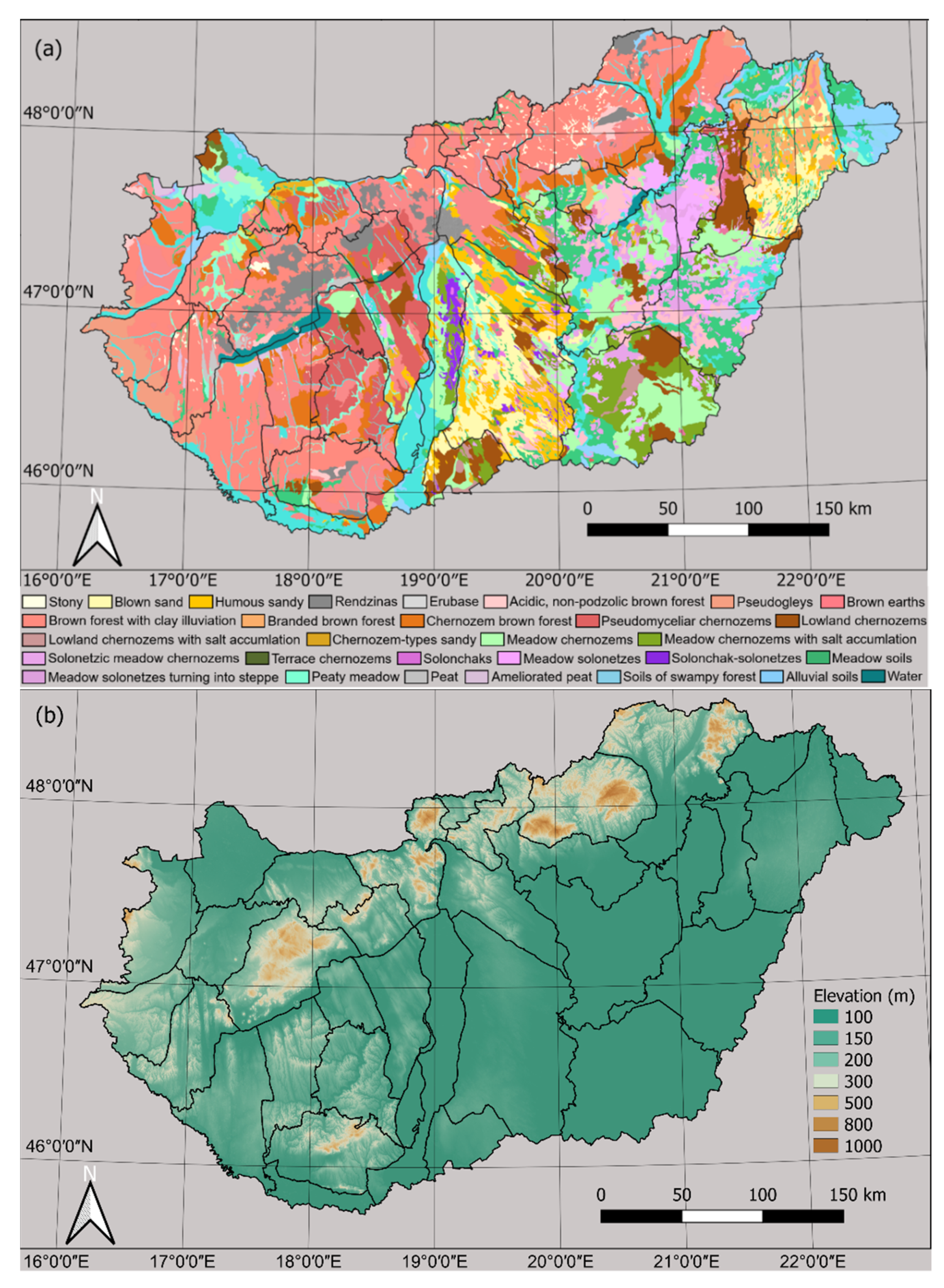
Our study area was the entire territory of Hungary, including all agricultural subsidy claims for the year 2020 and all available Sentinel-2 imagery between 1 January and 31 December 2020. Hungary has a temperate continental climate and relatively flat topography dominated by alluvial plains and loess, clay, or sand-based soils, ensuring favourable initial conditions for agriculture. Almost all major temperate zone plants can be grown, although frost, droughts, and flooding frequently affect yield negatively. Arable land covers approximately half of the country, dominated by cereal production (40%). Rapeseed (5%) and sunflower (11%) are also widely grown. Approximately 15% of cultivated land is occupied by grazed or mown grasslands. Hungarian farms are typically small in size, with 85% of farms and 83% of parcels below a total area of 5 ha and 10% of farms and 15% of parcels below 0.5 ha [
42]. Hungary was divided into 34 agro-ecological zones [
43] based on soils, topography, and climate (
Figure 1), and each of these zones was processed individually, with separate training and validation datasets within each zone, as recommended by Sitokonstantinou et al. [
2]. The number of parcels within each such zone varied considerably depending on the size and typical cultivation of the zone, from 4500 to 107,000.
Hungary is covered by four Sentinel-2 swaths, which means that, due to overlap between swaths from adjacent orbits, the revisit time can be increased compared to the single-satellite rate for large areas of the county. Generally, with Sentinel-2A and Sentinel-2B, most of the continental surface in Europe is revisited every five days under the same viewing conditions. Snow only influences data collection for a few weeks every year. On average, between 22 and 60 cloud-free Sentinel-2 images were available for each parcel in 2020.
2.2. Definition of Subsidy Monitoring as a Remote Sensing Data Analysis Task
The first step of remote sensing monitoring is to formally redefine the compliance rules of each individual subsidy category as criteria that can be checked with remote sensing. Remote sensing image analysis supports classification tasks (output is a crop class) and cultivation detection tasks (output is a cultivation action type and a time interval). Compliance to subsidy rules can be checked by defining a decision tree composed of individual questions that can be answered using satellite imagery.
Specifically, task 1 refers to the basic criteria defining agricultural cultivation (including temporary fallow land) under the SAPS. The positive rule of ground monitoring is that agricultural crops are grown on the area (or it temporarily functions as a fallow); negative rules are that water surfaces, built-up areas, forest, or other non-agricultural land use cannot be present within the parcel, and weeds and unmanaged woody vegetation may not be present either. In case the area is a grassland, a positive rule applies, stating that the area has to be mown or grazed. There is also a validity rule: the area has to be managed as a homogeneous unit with the same cultivation everywhere.
From a remote sensing perspective, the positive and negative rules may be checked using a vegetation classification approach where fallow land weeds and non-agricultural woody vegetation have their own category. The homogeneity rule can be checked relatively easily if a pixel-based approach is used. In our case, we opted for a polygon-based analysis, with the homogeneity criterion checked separately during parcel boundary evaluation at the preliminary check stage (not discussed in this paper).
Task 2 refers to the minimum criteria for grassland management under the SAPS. There are two negative rules for field monitoring of this funding scheme: overgrazing and overgrowth of non-grassland species (reeds, sedges) may not be present. Overgrazing is defined as “less than 50% of the surface of the parcel covered by vegetation due to grazing and trampling”. Reeds and sedges were included in the classification, while overgrazing had to be monitored specifically, by a dedicated analysis step.
Task 3 refers to diversification of crops within the land owned by each farmer. In this case, the diversification itself is checked at the database level from the submitted claims, while on-the-spot checks have the task to confirm that the crop grown at each specific site is the same as the crop claimed. Therefore, from a remote sensing perspective, this task has to be reduced to checking whether the claimed crops are truly present on the parcel. This can be solved by comparing the classification outputs to the claimed crop class.
Task 4 deals with sustaining grassland cultivation in environmentally sensitive areas. The single negative rule is that the claim is invalid if the parcel is ploughed, built in, or forested or the cultivation is changed in any way that is incompatible with sustained management as a permanent grassland. From a remote sensing perspective, this task can again be solved using a classification procedure: First, all parcels that are registered as sensitive grasslands are queried, and within this set, those not recognized by the classification as grassland will be considered non-compliant.
Task 5 refers to fallow land as ecological focus areas. Two negative rules define eligibility: no intensively cultivated crops can be present on the area between 1 January and 31 August, and no harvesting or mowing is allowed before 31 August. There is an exception to this latter rule: mowing is allowed for the purpose of suppressing weed growth. Classification of satellite imagery involves the class definition “fallow land”, and, additionally, mowing detection has to assess whether any cultivation event occurred before 31 August.
Task 6 is related to nitrogen-fixing crops as an ecological focus area. The rules related to this subsidy are that the crop cultivated on the area has to be one of the 40 crops listed as nitrogen-fixing, and that the crop has to be present on the field for a given period of time (depending on the type). Therefore, this task is redefined to checking whether the claimed crop class is truly present and detecting the time between sowing and harvesting in a dedicated step of analysis.
Finally, Task 7 is the mapping of catch crops as ecological focus areas. Catch crops are submitted as separate subsidy claims with their own geometry, together with sowing and harvest dates. According to monitoring regulations, whether a minimum of 60 days pass between the sowing and harvesting has to be checked. Remote sensing allows accurate determination of the harvesting date, but the sowing date can only be approximately derived between the harvesting of the main crop and the emergence of the catch crop.
All in all, each of these monitoring tasks can be solved if reliable vegetation classification is available and if agricultural cultivation events such as tillage and mowing can be detected. However, the level of detail of the categorization scheme will have a major influence on the reliability of the output.
2.3. Reference Data from Farmer’s Subsidy Claims
During the application process, farm owners draw parcel boundaries for each claim in an online system with georeferenced aerial photography as a background (
https://www.mvh.allamkincstar.gov.hu/e-ugyintezes, accessed on 15 July 2022). Crop types are selected from a list of registered crops, with additional cropping technologies related to ecological focus areas selectable as options (
Figure 2). Some ecological focus area conditions require the farmer to accurately report the time of cultivation activities, e.g., the sowing and harvesting time of catch crops. Farmer claims are expected to have about 2–3% errors (which is the reason for satellite monitoring), which limits the theoretical maximum accuracy that can be achieved when using them for training. Still, since countrywide training data with verified accuracy are not available, this information had to be used as a starting point. All in all, approximately 1,200,000 individual claims were submitted during the year 2020 in Hungary, and these datasets were our source of training and validation data (with the cutoff date of 29 December 2020), similar to [
2]. According to the experience of previous years’ on-the-spot checks, an error rate of 2–3% is expected, amounting to 25,000–35,000 false claims.
For the independent predictions for each farmer claim polygon, the claims of each agro-ecological zone were randomly halved, and one part was used for training and the other part for evaluation, and then the roles of these two parts were interchanged. For cultivation detection, sets of individual parcels were verified by manual interpretation and used as reference data for the training and validation process.
2.4. Satellite Imagery Preprocessing
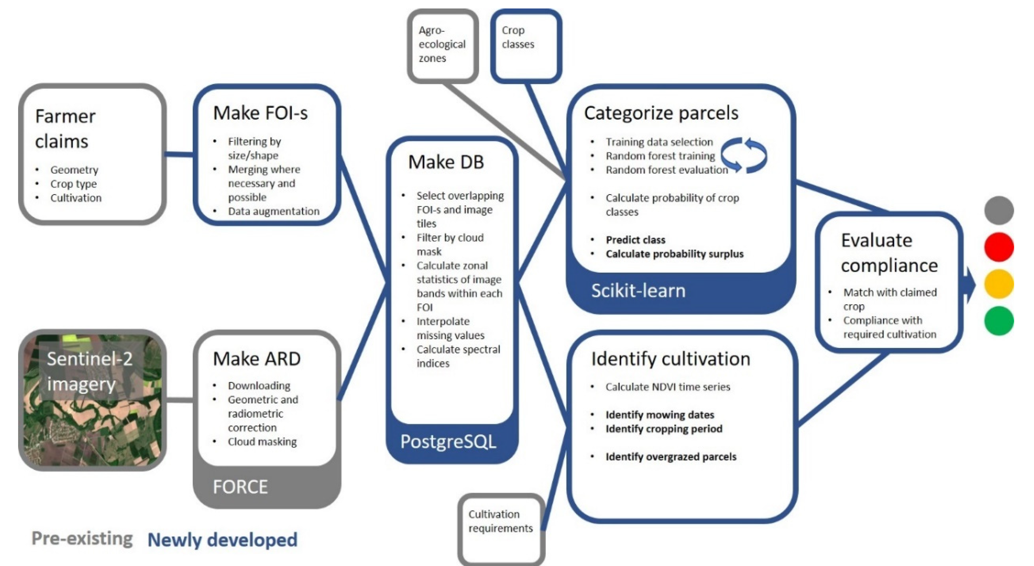
For this study, all available Sentinel-2 images (Level-1C) over the area of Hungary between 1 January and 31 December 2020 were downloaded from the European Space Agency’s (ESA) Copernicus Open Access Hub. Sentinel-2 imagery was pre-processed to the Level-2B processing level using the FORCE (Framework for Operational Radiometric Correction for Environmental monitoring) ARD (Analysis Ready Data) software (
Figure 2) [
17]. FORCE is a standalone solution for end-to-end processing of Sentinel-2 and Landsat data to create a harmonized, consistent set of imagery with common radiometric characteristics and spatial reference. FORCE cloud masking and atmospheric correction has performed well in comparison to other state-of-the-art methods [
45,
46] and is openly available. In our case, the processing pipeline carried out geometric correction, cloud masking [
47], and radiometric correction, producing modelled BOA (bottom-of-atmosphere) pixels.
2.5. Feature of Interest Preprocessing
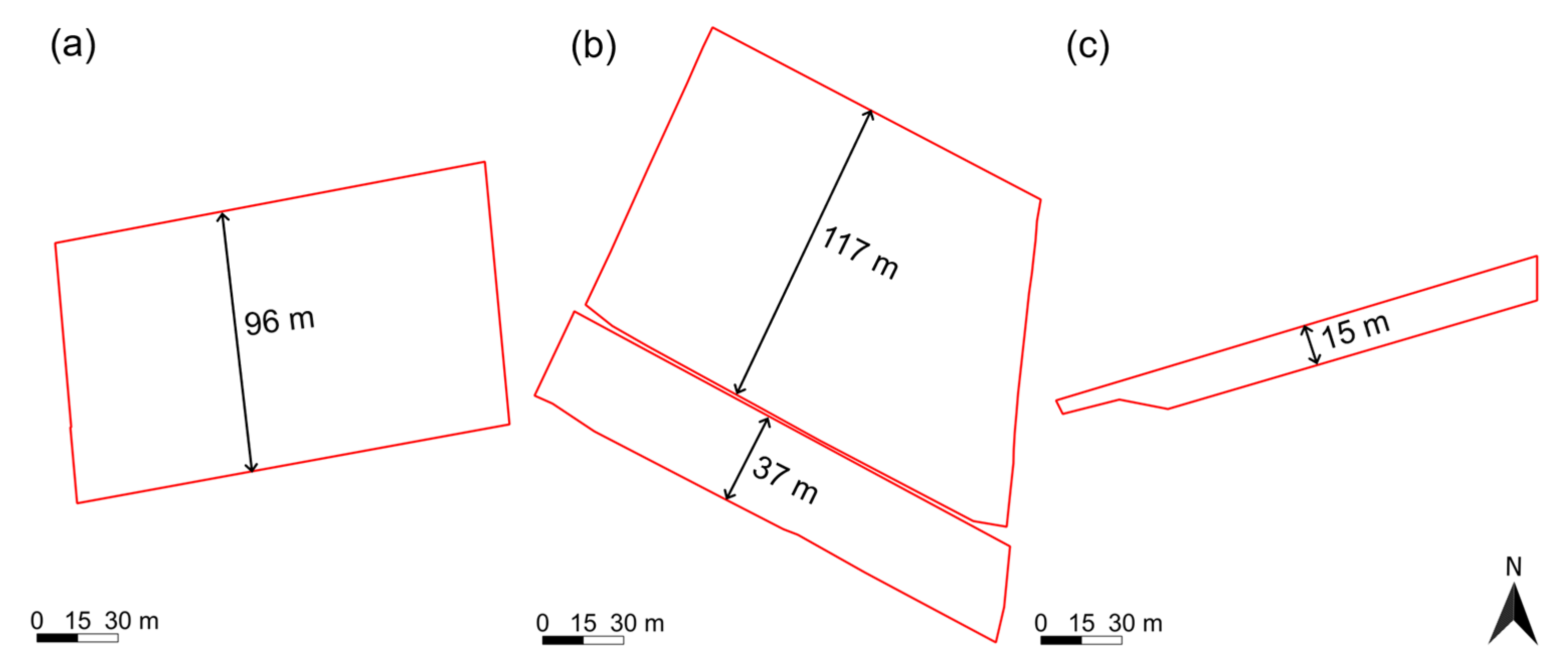
Target object size and shape often limits the application of satellite imagery [
48]. One possible workaround is the merging of adjacent parcels if they are covered by the same or similar crop type to form a single, larger feature of interest (FOI) [
34]. For our solution (
Figure 2), the first step was to select parcels that were large and wide enough to be analysed on their own: this was based on their area being larger than 40 m × the longest diagonal (straight line connecting two non-neighbouring vertices). The logic behind this is that, for a theoretical rectangular parcel, we avoid the pixels on the edges and want at least two pure pixels inside. Essentially, this means that rectangular parcels wider than 40 m were not merged. For parcels smaller or narrower than this, the neighbouring parcels were investigated. Neighbourhood was defined as the intersection after buffering of both geometries by 8 m. If another too-small parcel was found with the same vegetation class within this distance, the two parcels were merged by buffering with 5 m and then a negative buffer of 5 m applied to the resulting polygon (morphological closing) and their area-to-diagonal ratio recalculated. If the ratio was sufficient, the polygon was forwarded for analysis; if it remained too small, additional neighbours were searched. If no too-small neighbour could be found, neighbours of sufficient size were also checked for potential merging. All in all, 58% of all parcels were of sufficient size to be analysed on their own, and an additional 25% could be included after FOI merging, while 17% of the claimed parcels remained too small for analysis (
Figure 3).
Initially, Sentinel-2 FORCE tiles were assigned to parcel boundaries and cloud coverage was calculated for each. This resulted in a table connecting each parcel (by ID) with the Sentinel-2 image FORCE tiles (by acquisition date) that included the parcel geometry and were not covered by clouds. Afterwards, the rasterstats Python zonal statistics module was used to assign to each parcel the mean pixel values within their boundaries of each band and spectral index. During initial studies, a set of all spectral bands and several common spectral indices was tested for band importance in classification. Based on the outcome of this test, only the data products adding to the accuracy were kept and thus the following set was used: four selected Sentinel-2 spectral bands (Band 5: Red Edge 1, Band 6: Red Edge 2, Band 11: Shortwave Infrared 1, and Band 12: Shortwave Infrared 2); and five derived spectral indices (
Table S3): NDVI [
49], BSI (Bare Soil Index) [
50], EVI (Enhanced Vegetation Index) [
51], SIPI (Structure Insensitive Pigment Index) [
52], and YCI (Yellow Crop Index). YCI was purposefully designed for this study for selective identification of crops characterized by a yellow flowering phase (e.g., oilseed rape):
YCI returns a high value when both the red and the green channel are high and the blue is low—so when the surface is bright yellow. In all other cases, the index has lower values.
2.6. Random Forest Classification
Random forest (RF) was chosen as a classification method due to its robustness to errors in the training data and reasonable computation time [
53]. The RF classifier has been shown in earlier studies to yield excellent classification results and to successfully handle the high data dimensionality and multicollinearity of remotely sensed data [
54]. Additionally, the option for a fuzzy classification output was considered and extensively used during analysis. Fuzzy classifiers generate, for each classified unit, a vector of the respective probabilities of every class [
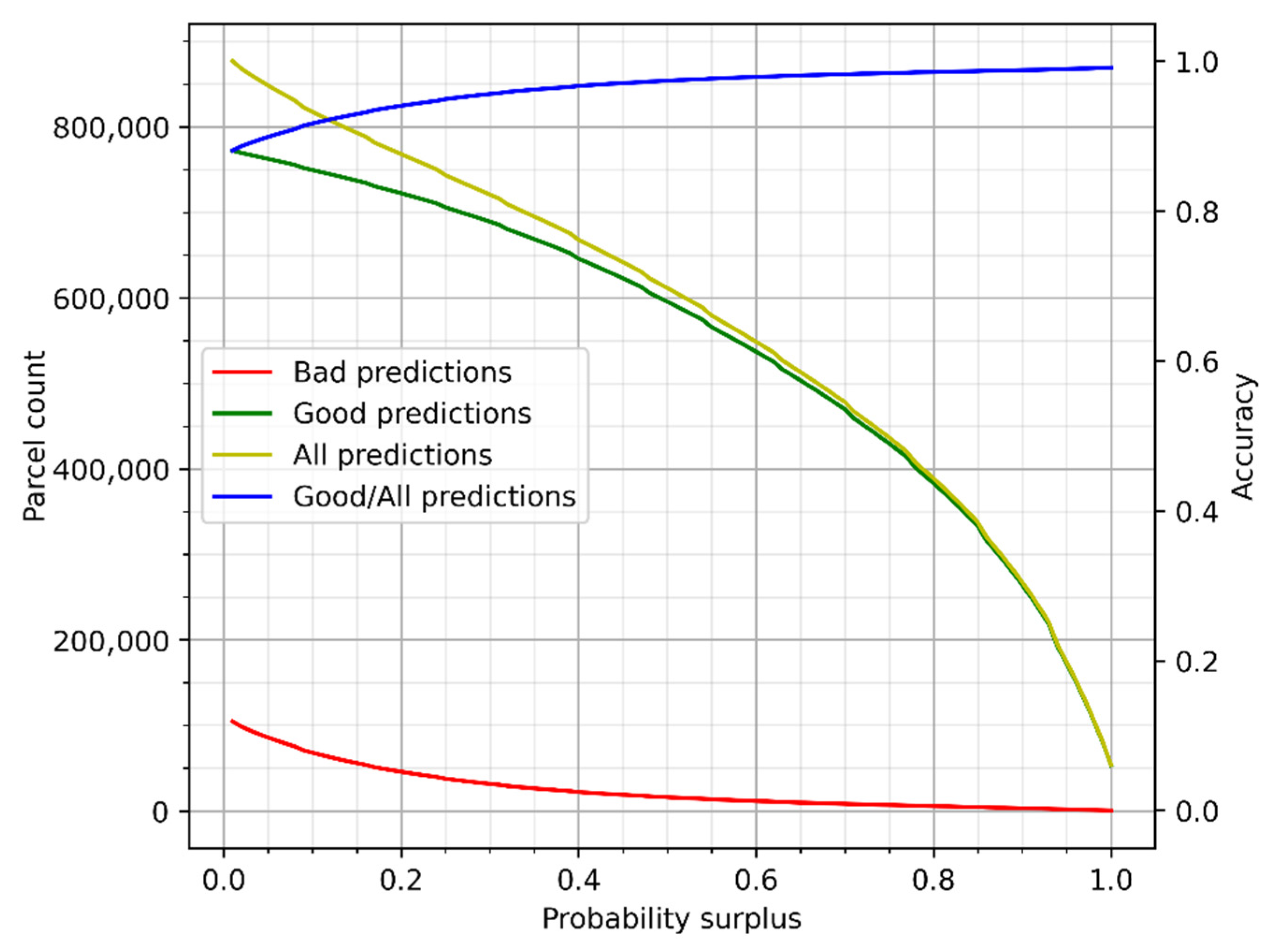
23]. On one hand, for specific vegetation classes, this output allowed including them in the evaluation even if they were not the dominant category (such as weeds or reeds); on the other hand, the fuzzy output also allowed calculation of a classification certainty metric for each FOI. Several such metrics are in use; we applied the probability surplus index [
55], also known in active learning as the “breaking ties index” [
56], as a direct representation of probability of the final class above the second-most-probable class—and thus the true certainty of the decision. Variable importance was calculated based on the impurity decrease, also known as a Gini importance [
53].
RF classification was implemented in the Scikit-learn Python module (
Figure 2) [
20]. Two parameters need to be set for RF: we set the number of decision trees to be generated (n_estimator) to 200 and the number of variables to be selected for the best split (max_features) to the square root of the number of input variables. The spectral data for each parcel with the indices was stored in PostgreSQL database tables (
Figure 2). The spectral index time series of the parcels were filtered by the agro-ecological zones—this was necessary to take the different soil and climate properties into account for the classification. The first step included a data-cleaning and systematization process: date and index pairs were created from the raw data and zero values were removed for all spectral indices, together with values larger than 1 or lower than −0.1 for NDVI. Empty dates were then filled in by linear interpolation between the value of the same spectral index on the preceding and following image. The SQL database table was read into a Pandas Dataframe object for data manipulation and analysis. Each FOI was represented by one row and n × m columns where n is the number of cloud-free measurements for the FOI and m is the number of spectral bands and indices in the RF classifier.
The set of individual parcels for each zone was split 50:50, ensuring that the individual classes were represented proportionally in both halves, A and B. In the next step, within one half of the dataset, 1% of the parcels were randomly selected within each class: this was the initial set of training data. This dataset was used to train the first classifier, and a prediction was made for all remaining data, within both the A and the B halves. Then, for each class within half A, 0.1% of the parcels were selected, those with the lowest probability surplus/breaking ties statistic, and added to the training dataset, labelling them according to the farmer’s claim. Then, the training and prediction was rerun, and again, the 0.1% of the parcels with the lowest probability surplus were added for each class. This was repeated until accuracy did not increase further for the next 15 iteration steps. Therefore, the number of parcels used for training within each class increased from typically 50–200 in the beginning to up to 1000–6000 in the end. In the final step, the resulting predictions were saved, but only for half B (which was not used as training data). The same process was repeated with training data selected from the B half and a final prediction made for the A half. Therefore, all parcels in each zone were predicted based on an optimized, relatively well-balanced set of independent training data. An example of the resulting map is shown in the
Supplementary Material.
One output of the RF classification was a database table with probabilities for each vegetation class, probability surplus values, and predicted classes for each FOI. The other output was a text report file which included a detailed list of the variables and imagery dates used (ordered according to their importance), the iteration steps and their overall accuracy, and the precision and recall values for each class (similar to Vegetation Classification Studio, [
57]). These report files were highly useful for comparing the results of individual classification and optimizing parameters.
2.6.1. Definition of a System of Vegetation Classes
During initial tests, it was found that the system of classes used has a strong influence on classification accuracy. Ideally, every cultivated crop would be a class of its own, but since a lot of crops are spectrally similar, this is not possible and they have to be grouped [
13]. Crop classes are expected to be spectrally homogeneous during the growing season and form relevant groups for subsidy monitoring purposes. This already has its limitations, since some crops are sown either in autumn or spring and others are cultivated for several years but in the initial phase have completely different spectral characteristics than at their mature phase (e.g., alfalfa, but also energy coppice). Additionally, grasslands and fallow land can be quite heterogeneous within the same parcel, and, for fallow land, the vegetation growth will heavily depend on the crops of the previous year. Crops that have a short growth period may result in bare soil conditions for several months during the year, where the soil properties will strongly influence the spectral response. Finally, care had to be taken to ensure that every crop encountered will fall into a meaningful class from the perspective of subsidy monitoring (no “other” class could be defined), keeping in mind that non-crop land cover may occur within claimed areas and this will influence classification accuracy [
58]. Crop classes were iteratively refined based on the outcomes of initial test classifications and evaluated using dominance profiles [
55] and confusion matrices, in addition to information on growth characteristics and cultivation practices.
The final system of classes includes the following (
Table 1):
Maize (including regular and hybrid corn, but not maize grown for silage).
Winter cereals (mostly winter wheat, winter barley, and winter triticale).
Grasslands (including temporary and permanent grasslands and both mowing and grazing as cultivation, but also green manures if they include grasses and traditional orchards, as they have larger surface cover of grassland than of the trees themselves).
Sunflower (hybrid and regular).
Alfalfa (including newly planted and regularly cropped fields but also alfalfa grown in combination with grasslands).
Fallow land (land temporarily left uncultivated with no tillage, sowing, or mowing before 31 August in the given year).
Grapes (wine and table grapes).
Rapeseed (mainly autumn but also rarely spring).
Tree plantations (orchards, artificially planted trees for energy, or lumber—mainly apples, cherries, or poplar trees).
Spring cereals (mainly spring oats, barley, and Sorghum).
Vegetables and strawberries (dominated by mixed vegetable gardens but frequently also pepper, pumpkins, and cabbages).
Soybeans.
Weeds (croplands covered by non-cultivated nuisance vegetation. Ground truths for this class originate from on-the-spot-checks).
Field vegetables. These are herbaceous plants grown for their seeds, fruits, or tubers, planted as seeds (tubers) and harvested by machinery. Introducing this class was found necessary due to the spectral differences compared to vegetables planted as seedlings and harvested by hand. Typical crops for this class include potatoes, green peas, oilseed pumpkin, and carrots.
Fodder plants (excluding alfalfa but including both mono- and dicots and annuals and perennials. These are herbaceous monocots or dicots grown for their biomass and harvested while green. Typical examples are silage Sorghum and Setaria, but also bee plants such as Phacelia).
Forests (dominated by trees growing in a semi-natural, non-systematic pattern. Newly planted forests are included in the fallow land class).
Herbs and spices (herbaceous plants grown not for their biomass or fruit, including ornamental plants, poppy seed, lavender, and fennel).
Sugar Beet.
Rice (regular and wild rice).
Shrub crops (woody stem, branching directly above the ground, free standing, or trained on wires—typically elderberries or blackberries).
Reed (both cultivated and uncultivated reed, together with wetland reconstruction).
Fiber plants (hemp, flax, sorghum).
Energy plants (herbaceous, tall-growing monocots or dicots grown for their biomass but harvested after drying—Miscanthus, Arundo donax, or other grasses).
Other—non-crop land cover (water, bare soil, sealed surfaces).
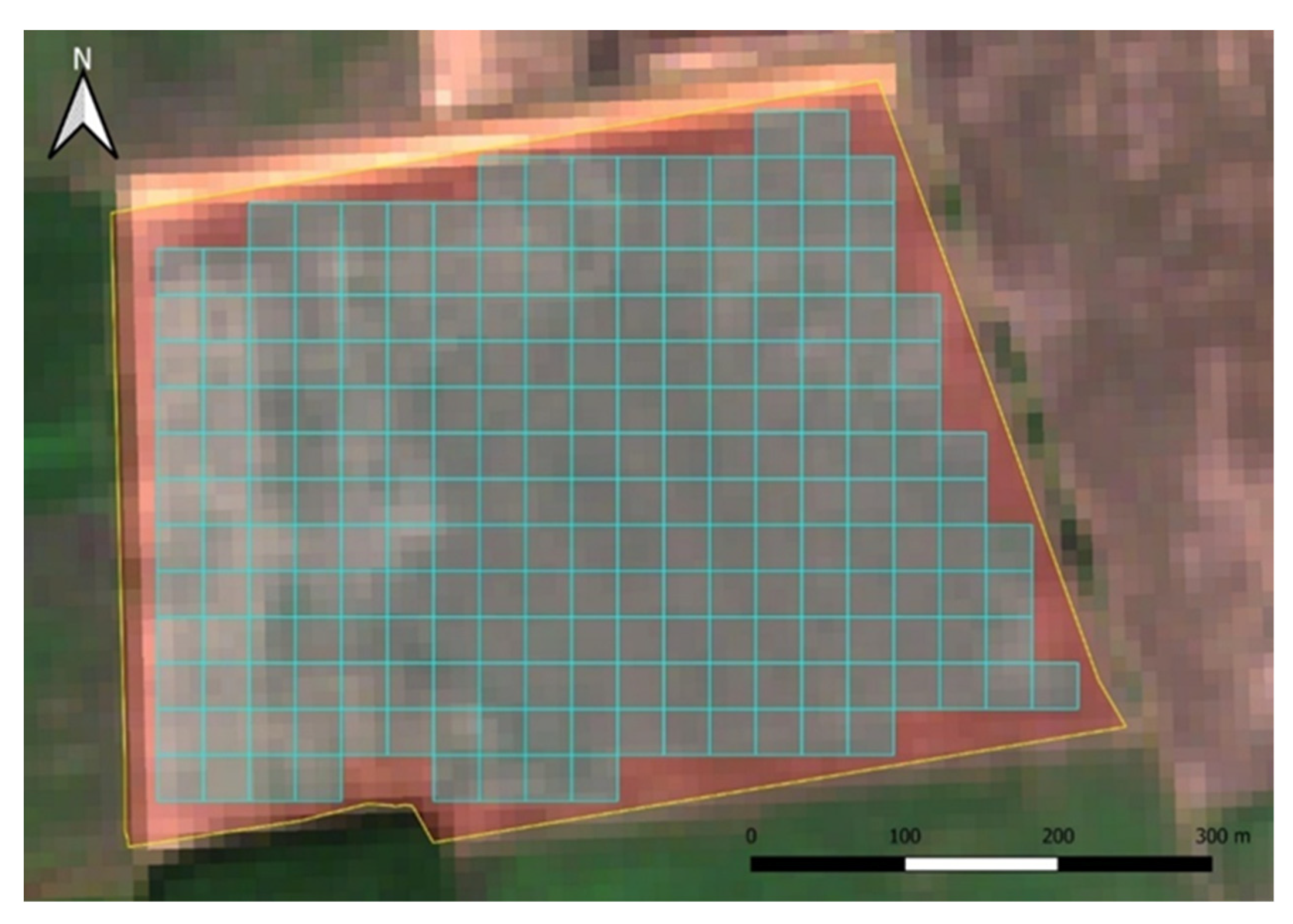
Apparently, some of the classes here contain several orders of magnitude more parcels than others, resulting in an imbalanced classification. In practice, this means that parcels belonging to very rare classes will be more frequently misclassified, often as belonging to one of the most dominant classes (typically maize). In addition, some categories never occur in farmer subsidy claims as they are ineligible for funding and represent mismanagement, but still exist in the field and have to be identified. For these classes, evidence exists from on-the-spot checks, including spatial outlines, but such cases are rare. In order to increase the number of reference data available for training, these categories were differently handled than regular training data from farmer claims, applying a simple data augmentation technique. In data augmentation, it is a priority to preserve the original properties of the target as far as possible while increasing the number of distinct cases [
59]. Instead of entering each parcel as a single entity with its mean spectral indicator values, such parcels were split into smaller units of 30 × 30 m, and these smaller units treated as if they were individual “parcels” (
Figure 4). Therefore, the mean spectral values were calculated separately for each sub-unit and they could be used for training and evaluation. This way, the number of data points could be increased by approximately an order of magnitude for these underrepresented classes, while still using image data from verified locations—similar to the “hide-and-seek” data augmentation technique [
60] but without the spatial dimension, since the parcel itself is the unit of classification. The disadvantage of this approach is the spatial autocorrelation between the samples that constrains their independence.
2.6.2. Evaluation of Classification Accuracy
Classification accuracies were evaluated using confusion matrix indices, with overall accuracy as the main metric optimized during iterations. The results of individual agro-ecological zones were compared by evaluating the full matrix (
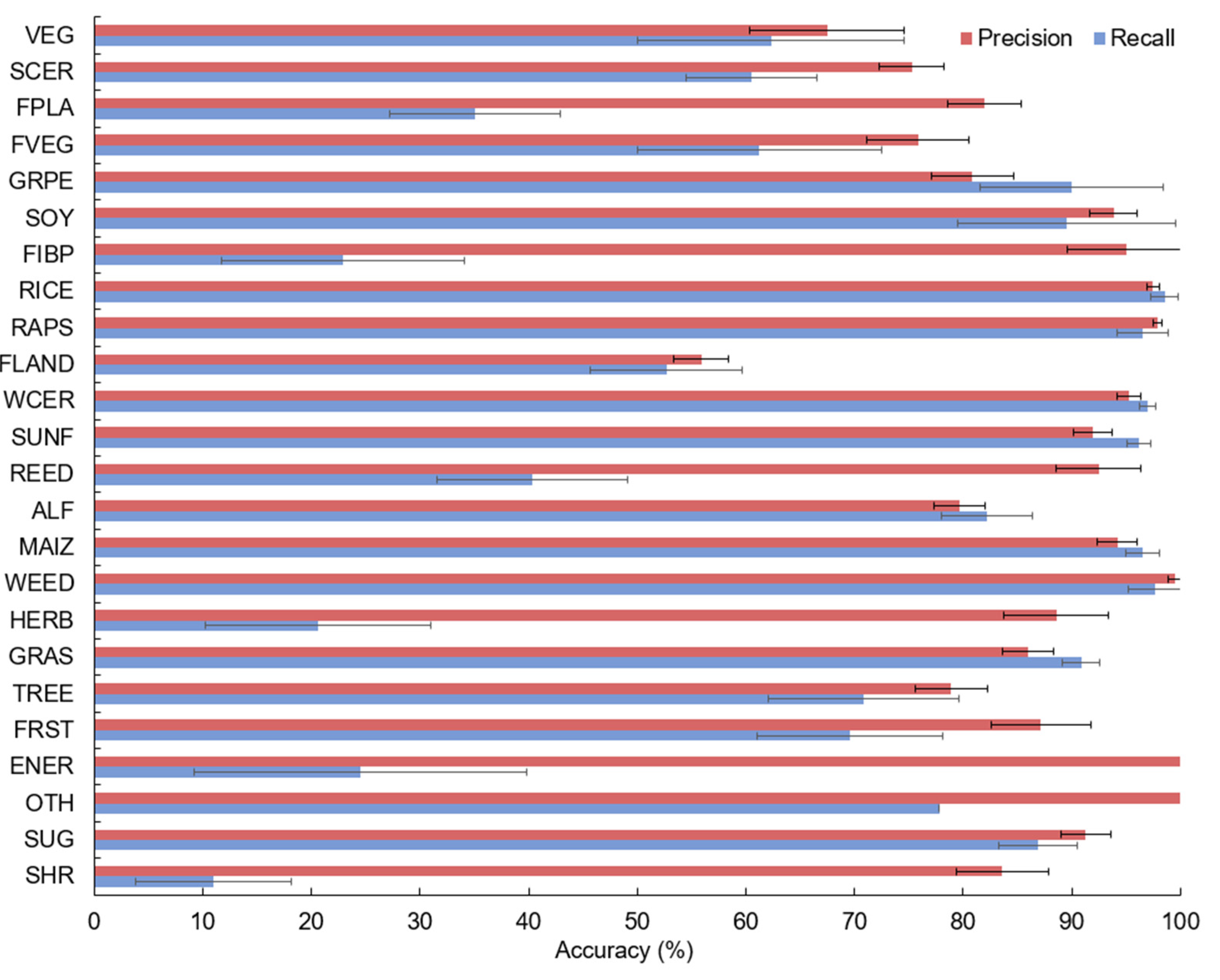
Table S1). Accuracy per class indices such as precision and recall were complemented by standard deviation values calculated from the accuracies of the same class within the individual zones. Therefore, the variability or confidence of these metrics can also be quantified (
Figure 5). The Matthews Correlation Coefficient (MCC) was calculated because it is increasingly used in machine learning and is thought to be a sensitive and robust indicator of classification accuracy [
61].
In order to better understand the characteristics of each class, dominance profile plots were also generated [
55]. In the final step, the paying agency has to decide which farmers to select for further notifications or field checks based on non-compliance identified with high certainty. This was carried out by creating a cumulative histogram of false and true claims ordered by the probability surplus metric, showing how many identified non-compliant claims would result at each cut-off level of probability surplus (
Figure 6). Evaluating this graph allowed selecting a relevant number of non-compliant claims that are probably unaffected by classification errors.
2.7. Detection of Cultivation Event Dates
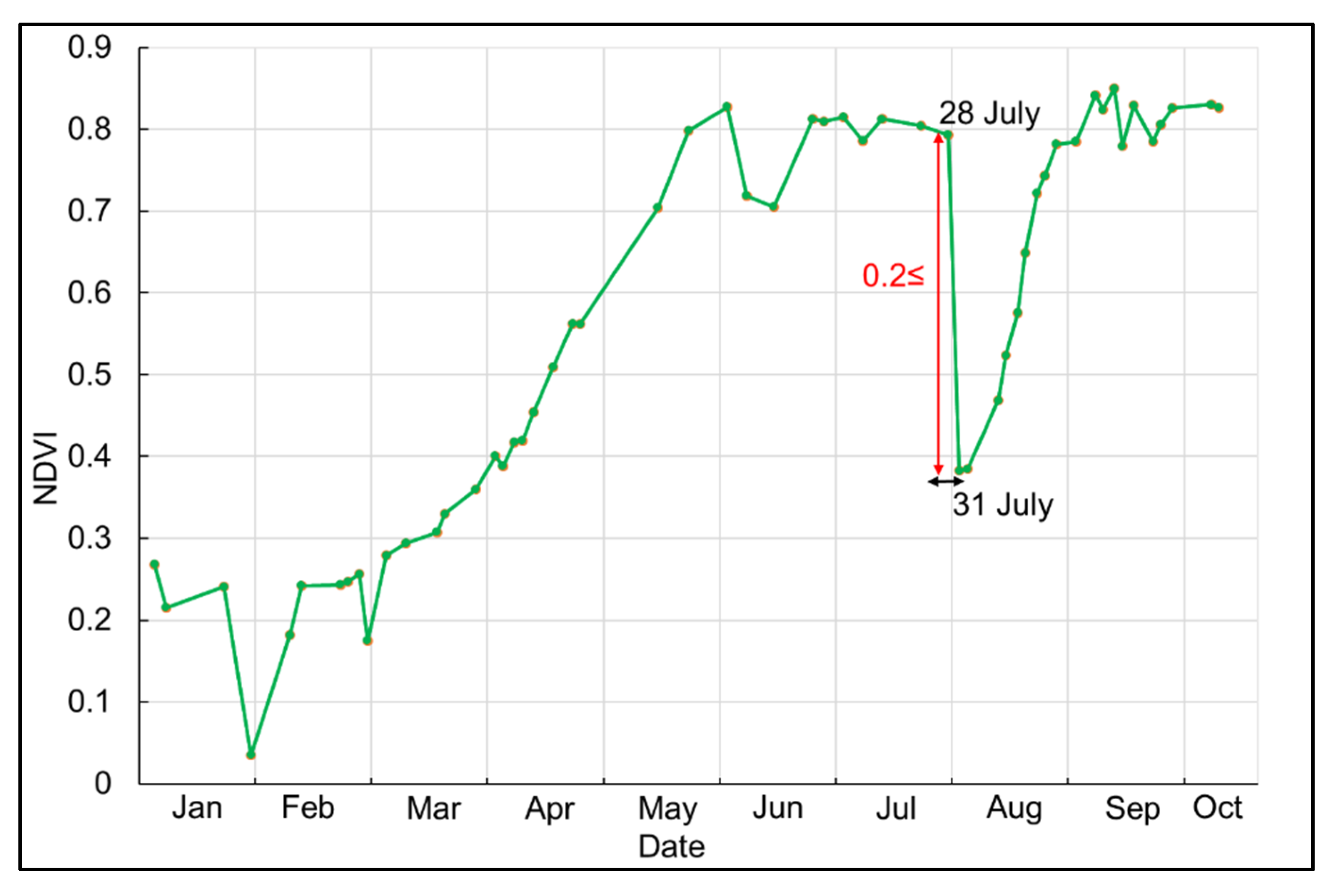
Mowing was detected based on the algorithm of Kolecka et al. [
25]. A parcel was registered as mown in a certain period if the mean NDVI of a parcel decreased more than 0.2 between two subsequent cloud-free observations or the first and last of three subsequent clear observations (
Figure 7). Mowing detection was carried out for parcels where the reference or the predicted class was grassland, fallow land, alfalfa, or forage crop. Mowing events generally take place after 1 April in Hungary and parcels are often affected by snow or inland excess water before this time period. Therefore, NDVI drops of more than 0.2 were identified as mowing only after 1 April.
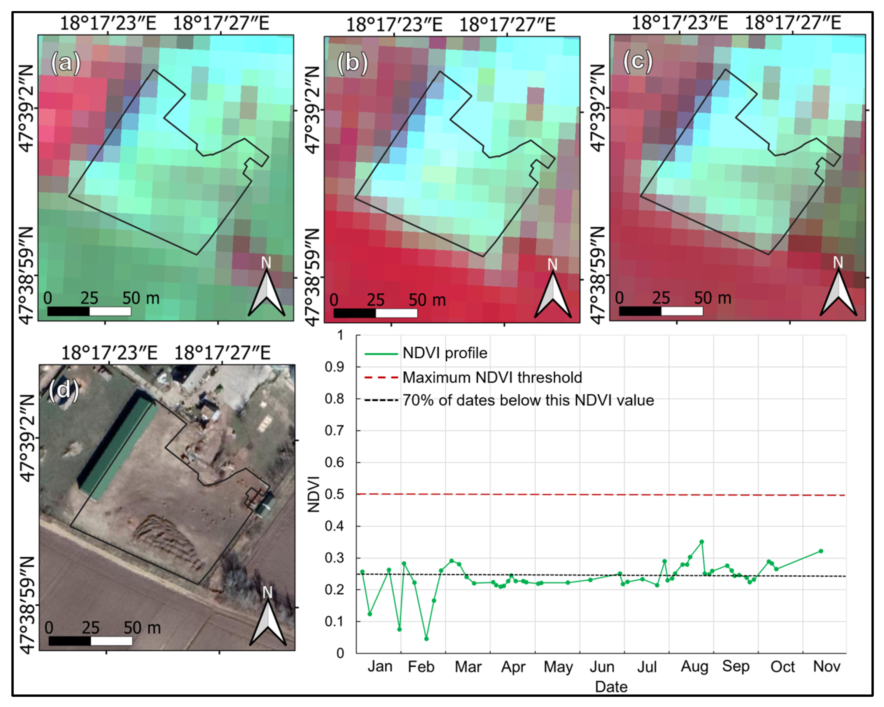
2.8. Detection of Grassland Overgrazing
Overgrazed areas were delimited based on reference data from the field checks performed for subsidy controls; however, such cases are very scarce. Only 8 parcels were classified as overgrazed on the field check, which was not sufficient as training data for a classification procedure. Therefore, after visual inspection of the identified overgrazing locations and the NDVI time series data, the following ruleset was defined: a grassland parcel is overgrazed if the maximum of the mean NDVI value is below 0.5 and remains below 0.25 on at least 70% of the image dates from a year (
Figure 8).
2.9. Detection of Cultivation Time Period and Catch Crops
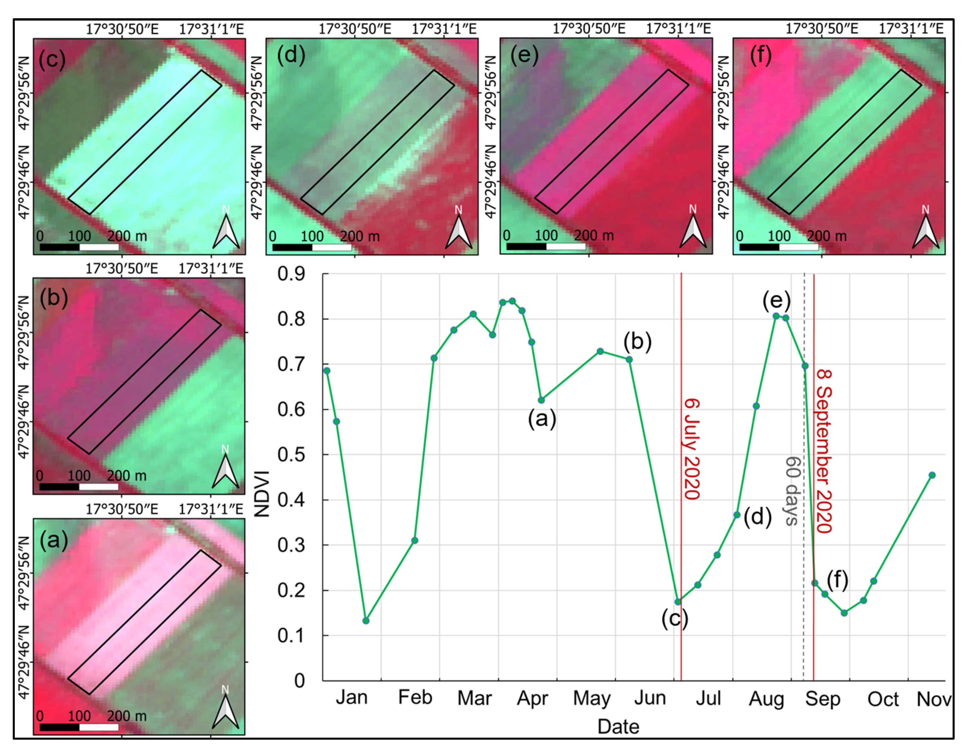
Nitrogen-fixing crops have specified cultivation periods depending on crop types (e.g., alfalfa from 1 May to 30 September), and catch crops are required to be on site for 60 days from sowing to harvest or tillage. These intervals were again checked based on the NDVI time series of each parcel. Catch crops may be cultivated in a spatial layout different from the original parcel boundary but the catch crop boundary also has to be reported by the farmer, together with the actual date of sowing and removal of the vegetation growth (typically by harrowing, but also mowing). Therefore, this additional set of polygons was processed via FOI generation and spectral index statistics calculation. We investigated the NDVI time series by first identifying the maximum and minimum values and their respective dates between the reported start and end of catch crop growth. Any NDVI values not more than a selected threshold (0.075) above the minimum were considered to correspond to bare soil. The time interval of the catch crop was calculated from the first date when bare soil was registered before the minimum to the first date when bare soil was detected after the maximum (
Figure 9). If the time difference between these two dates was more than 60 days, the parcel was confirmed to have passed the requirement. If the interval was between 56 and 59 days, the parcel was classified as uncertain, while if the difference was no more than 55 days, the parcel was marked as failed.
Information on cultivation events was validated using a purpose-built QGIS plugin that allowed for visualization of satellite imagery together with the Geospatial Aid Application (GSAA) database geometries and attributes. The accuracy of mowing detection was evaluated on a total of 160 parcels, with at least 30 parcels for each relevant vegetation class (alfalfa 10 samples) from one selected agroecological zone. Negative control samples were also selected for grassland and fallow land categories (GRAS_NM and FLAND_NM) to detect false positive errors.
2.10. Rulesets for Monitoring Individual Tasks
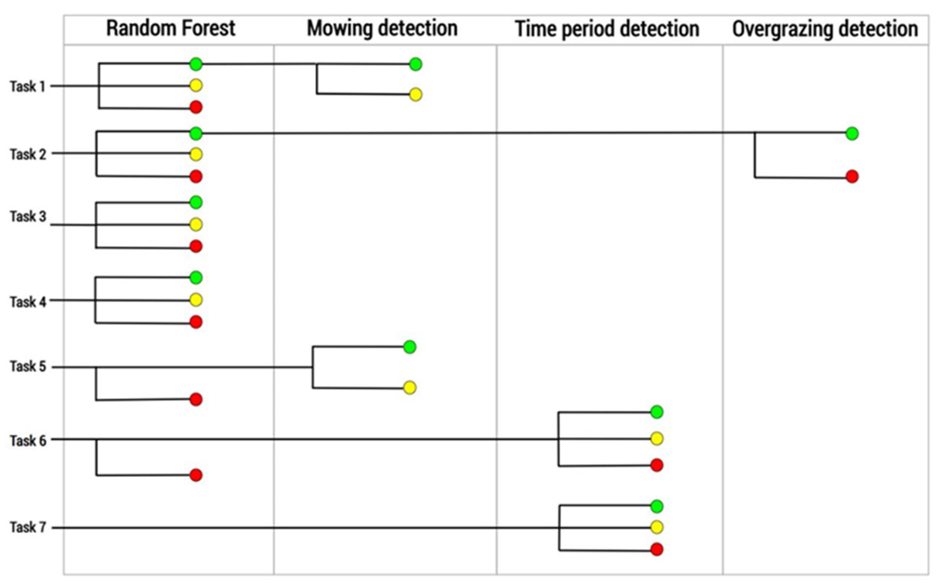
For each specific monitoring task, a set of rules was developed in the form of a decision tree that defined which information had to be queried from the claim database, what remote sensing products were to be used, and which outcomes resulted in a valid, invalid, or uncertain claim (
Figure 2 and
Figure 10).
For task 1 (detection of basic cultivation) we assumed that all parcels are eligible where the presence of a crop can be proven. Grasslands are a special case since they are eligible only if actively grazed or mown or if not dominated by weed vegetation. Therefore, the first step was to evaluate the result of vegetation classification. If a parcel was claimed as a crop, and the classification output was not “grassland”, “fallow land”, “weeds”, or “reed wetland” (which can be cultivated, but is ineligible for CAP support), then the parcel was evaluated as correct (green). If a parcel was claimed as a crop, but the “weed” class was found to be dominant, then the parcel was registered as ineligible (red). However, for non-grassland parcels, regardless of the claim, if the probability of weeds was above a certain threshold (20%), the parcel was registered as uncertain (yellow) and listed for further checking. For parcels claimed as mown grassland or fallow land identified by satellite imagery classification as grassland, in the second step, mowing detection was applied and if a mowing date could be ascertained, the parcel was evaluated as eligible regardless of the weed probability. This approach was chosen because the accuracy of mowing detection was better than the accuracy of the weed class.
For task 2 (minimum criteria for grasslands), we checked all parcels that were claimed as mown or grazed grassland. If imagery-based classification identified the parcel as “reed” or “weed”, it was registered as ineligible (red). If the parcel was identified as grassland, overgrazing detection was the next step. If overgrazing was identified, the parcel was also registered as ineligible (red). Furthermore, the probability of reed (or other non-cultivated grassland vegetation) was assessed from the classification: if the reed or weed probability was above 30%, it was assigned to the “uncertain” (yellow) class. If the parcel was assigned to any other class (including woody vegetation or arable crops), task 2 was not further investigated.
For task 3 (crop diversification), the question to be investigated with remote sensing was whether the crop claimed by the farmer corresponds to the crop class identified from image classification. If the classification found the claim to be correct, the parcel was registered as eligible (green) from a crop diversification perspective. If the claimed crop and the identified vegetation class were found to contradict, the parcel was assigned to the “uncertain” (yellow) class within task 3 as this required follow-up. No parcel was assigned to “non-compliant” (red).
Task 4 (maintenance of sensitive grasslands) combined a dataset of the paying agency (containing all parcels listed as sensitive grasslands) and the result of the classification. If a sensitive grassland parcel belonged to the “grassland” class, it was registered as eligible (green), if it was in the “fallow land” class, it was registered as uncertain (yellow). If any other class was present, this was taken as a sign that the grassland was converted to a different cultivation and the parcel was marked as ineligible (red).
Task 5 (fallow land ecological focus areas) was also based on the outcome of vegetation classification and mowing detection. According to greening rules, set-aside land is eligible if there is no intensively cultivated crop on the parcel and it is not mown before 31 August. Due to the difficulties of separating fallow land and grassland in the classification, both classes were considered eligible (green) if no mowing was detected before 31 August. If mowing was detected before this date, the parcel was counted as uncertain (yellow). If a different vegetation class was detected (not grassland or fallow), the parcel was registered as ineligible (red).
Task 6 (nitrogen-fixing crops) was solved based on the claim, the output of vegetation classification, and time period detection. However, nitrogen-fixing crops fall into several vegetation classes (alfalfa, forage crops, vegetables etc.), therefore it was not possible to use only the classification output. If the claimed crop was in the list of nitrogen-fixing crops and the predicted class corresponded to the vegetation class of the claimed crop, the parcel was found eligible (green); otherwise, it was ineligible (red). If the crop was present on the field for the required period of time, depending on the type, the parcel was found eligible (green); otherwise, it was uncertain (yellow) or ineligible (red), depending on whether the NDVI value dropped below 0.3 or 0.25 at the time of cultivation. However, if the decrease in NDVI was followed by a sudden increase within three weeks, it was considered mowing, which is allowed in the regulation.
Finally, for Task 7 (catch crops), only the cultivation time detection algorithm was used. The output was a set of two timestamps for the start and end of catch crop cultivation: if the difference between them was longer than 60 days, the parcel was found eligible (green); if it was between 56 and 59 days, the parcel was uncertain (yellow); and if it was shorter than 55 days, the parcel was ineligible (red). If there were not enough cloud-free measurements to determine the length of cultivation, it was classified as uncertain (yellow).
3. Results
Specifically for individual tasks, the accuracy and utility of remote sensing monitoring was found to be variable, but for the overall set of operations, the efficiency was clearly comparable to or even better than field checks. First of all, parcel detection and FOI generation with the defined minimum size found 83.5% of the parcels available for monitoring and the rest to be too small or narrow. This resulted in approximately 1,000,000 parcels that were the subject of further remote-sensing-based analysis and about 200,000 that had to be excluded; but when converted to area, this means that 97% of agricultural land in Hungary was successfully monitored. Merging of similar neighbouring parcels into features of interest allowed including more than 300,000 additional parcels that were below the size limit on their own (
Table 2).
Feature importance assigned to the individual spectral bands and indices had limited variability between zones: standard deviations of feature importance between zones were typically around 10% of the importance of each feature. Band 6 (Red Edge 2) had the strongest contribution to classification accuracy, followed by NDVI and Band 5 (Red Edge 1), Band 11 (Shortwave Infrared 1), and SIPI, BSI, EVI, YCI, and Band 12 (Shortwave Infrared 2). The importance of images by date showed two peaks typically, one at late spring (end of April—beginning of May) and another in summer (end of July typically).
The overall accuracy of the RF classification was 88.07% (
Table 3 and
Table S1), (MCC was 0.87) with rice, maize, and oilseed rape reaching classification accuracies above 95%; weed-dominated areas, grasslands, soybeans, and grapes with accuracies at or above 85%; and sugar beet, non-crop land, and reeds above 75%. However, the non-crop land class and especially the reed class were substantially overestimated, together with forage plants, as shown by the precision being far higher than recall. The lowest accuracies were observed for shrubs (11%, mainly misclassified as trees, grassland, or grapes), energy crops (23%, most frequently mapped as grassland), herbs and spices (19%, misclassified as fallow land or vegetables), and fibre plants (24%, misclassified as maize, sunflower, or soybeans). These latter classes were also overestimated. All in all, the most frequent classes were reliably identified, and misclassifications mainly affected underrepresented classes (
Figure S3). The variability in crop class accuracies between agro-ecological zones is remarkably low for most well-identified classes but is somewhat higher for rare classes. This suggests that the number of parcels or the ratio of these rare crops varies significantly between zones, with the sparse cases providing low accuracies and the zones where these crops occupy significant area providing better accuracies. Comparing the confusion matrix calculated from all parcels with the “model accuracy” calculated based on 1000 randomly selected parcels from every class (
Table S2), the overall accuracy figures are significantly lower (OA 0.72, MCC 0.70), but the relative accuracies of the individual classes are remarkably similar, suggesting that the high accuracy of the dominant crop classes is independent from their frequency.
From the perspective of misclassified parcel counts, the most numerous errors were mapping fallow land as grassland, grassland as alfalfa, or alfalfa as grass. Since alfalfa–grass mixtures are widely cultivated and vary strongly in terms of dominant vegetation, even within a single parcel, this error is difficult to resolve without a more rigorous definition of classes. Similarly, fallow land vegetation often transitions towards grasslands; therefore, this error is also difficult to resolve. Grasslands and fallow also produced misclassification errors to other categories: trees–grasslands and grassland–fallow were relatively frequent errors (up to 3500 parcels affected). Misclassifications between summer cereals and maize, maize and sunflower, or summer cereals and winter cereals are less expected and more likely to occur due to error in submitting the claim.
The accuracy was found to correctly identify mowing or lack of mowing with 86.0 and 86.7% respectively (MCC 0.71) (
Table 4). Main sources of error were the aggregation of parcels with different mowing dates to a single FOI or the inaccuracies of the cloud mask.
A total of 151 overgrazed parcels were found using the NDVI time series thresholding. The accuracy of overgrazing detection was evaluated by visually checking all of the 151 parcels on Sentinel-2 and Google Earth satellite images. This check found 63.7% of the parcels to be correct.
For nitrogen-fixing crops, the cultivation time was evaluated separately for alfalfa (which is the most frequent class) and other nitrogen-fixing crops. For both classes, 25 cases were selected randomly where cultivation time was found compliant to regulations and 25 where the cultivation was too short—altogether, 100 parcels were investigated in this balanced setup. For alfalfa, the overall accuracy was 84%, while for the other crops, it was 77%. For this latter group, all test cases of insufficient cultivation length were correctly identified while approximately 30% of the sufficient reference cases were misclassified as too short. The catch crop cultivation time detection method was evaluated compared to 100 hand-interpreted catch crop parcels, selected to ensure 50% passed and 50% failed. The overall accuracy of detecting correct or incorrect management was 88.7% (MCC 0.77) for this selection (
Table 5).
Task 1 involved all subsidy claims (except cultivated reed) independently from the crop, more than 1,200,000 parcels altogether. Based on the identification of basic cultivation criteria, the overwhelming majority of the parcels was found compliant (99.55%) (green), with 0.13% uncertain (yellow), and 0.32% ineligible (red).
Task 2 (minimum cultivation of grasslands) affected all parcels claimed as mown or grazed grassland, 160,663 units altogether. Of these, 99.5% were confirmed to be correct (green), only 4 parcels were uncertain (yellow), and 0.5% were ineligible (red)
Task 3 involved all farmers who claimed more than 15 ha in area (from several parcels). Slightly more than half of the parcels had to be investigated (734,460 parcels). Since control of crop diversification is not possible by remote sensing alone due to the high number of classes and the connection to former years, for this task, only correct or uncertain results were registered, based on the agreement between the claimed crop and the vegetation class found from remote sensing. However, the accuracy of the classification has a strong influence on the outcome of this task, since all parcels with a mismatch between the claimed and identified class were registered as uncertain. All in all, 10.4% of the parcels were found to be uncertain and 89.6% were correct.
Task 4 involved only sensitive grasslands and therefore a relatively small number of parcels (50,650). For 97.2% of these claims, eligibility was confirmed, but 2.5% of the parcels were found to be non-compliant (red) and 0.3% were uncertain.
Task 5 represented uncultivated parcels as ecological focus areas, which include 37,002 parcel units altogether. For these cases, identification of grassland or fallow land use proved problematic, and for many of them, mowing was also detected earlier than allowed. Correct cultivation was only registered for 30.6% of the parcels, 41.3% were found to be uncertain (yellow) mainly due to detected mowing, and 28.1% were incorrect (red), where the dominant vegetation was not “fallow land” or “grassland”.
Task 6 was the identification of nitrogen-fixing crops and their cultivation time and therefore affected an even smaller fraction of the parcels: 28,054 claimed parcels were investigated based on both crop classification and cultivation time. 71.4% were found correct and 21.7% incorrect, and 6.9% were identified as uncertain. The accuracy of the crop type classification has a strong influence on this task, since 18.9% of the parcels were registered ineligible due to the misclassification between vegetation classes.
Task 7 was the checking of catch crop parcels, and included only a small fraction of the total dataset: 25,503 claims. Results were similar to the previous task: 81.9% were correct, 5.3% uncertain, and 12.8% ineligible.
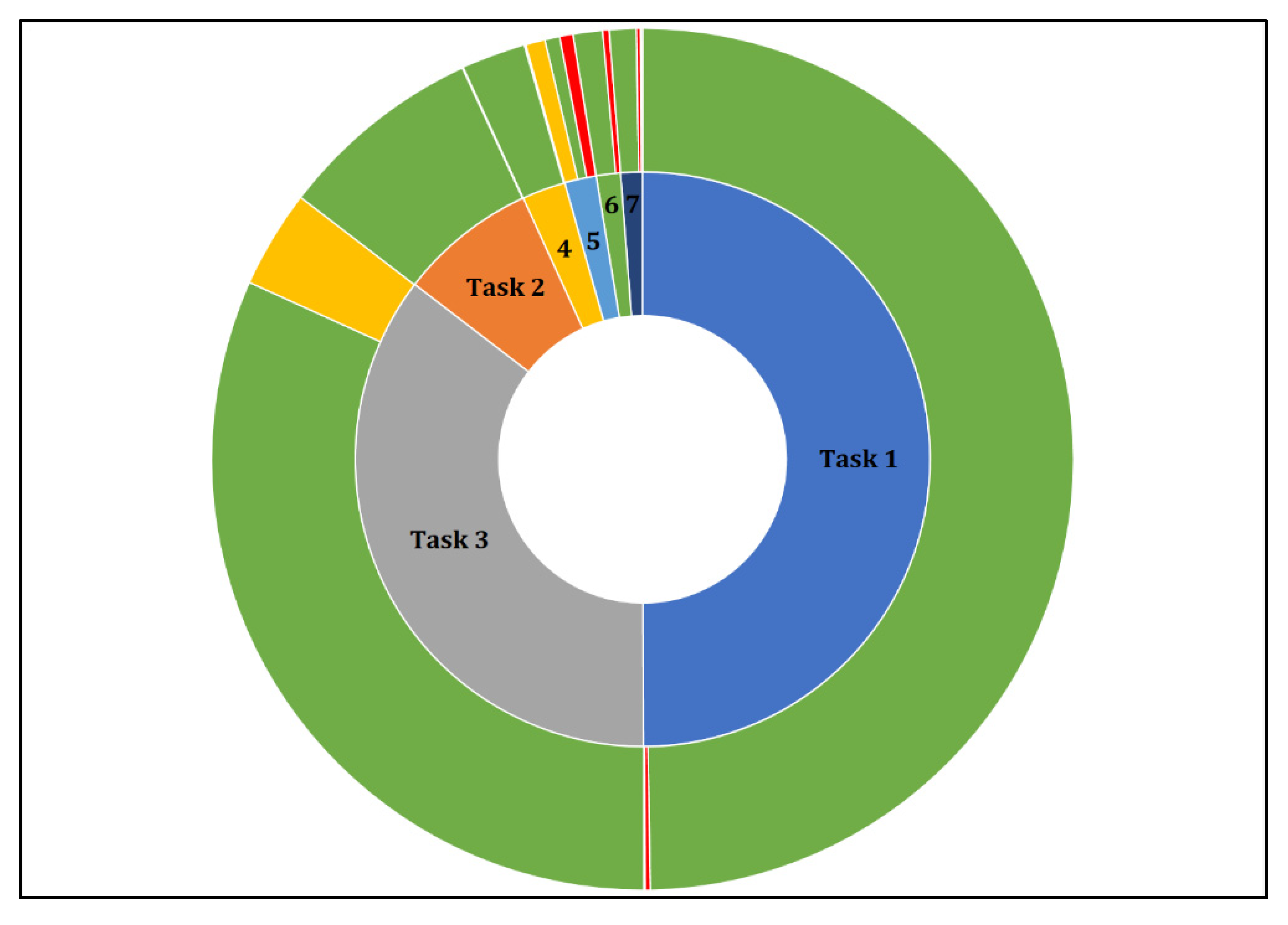
Altogether, more than 2 million monitoring operations (individual combinations of parcel and task) were completed. Most of these belonged to task 1 and task 3, as these had to be performed for all crop types, and smaller amounts to tasks 2, 4, 5, 6, and 7, as these belonged to individual crop classes. 94% of these operations resulted in the claim being confirmed as eligible, 1.5% identified erroneous, ineligible claims, and the rest (4.5%) remained uncertain and require investigation with different methods, including (but not necessarily limited to) field visits. Most of the inconclusive results were produced by disagreement between the claimed crop and the mapped vegetation class for task 3 and classification errors influencing task 5.
At the parcel level, 90% of the parcels was assigned only eligible (green), 7.9% identified uncertain (yellow) for at least one of the tasks but not ineligible (red), and the rest (2.1%) registered erroneous (red) at least once (
Figure 11).
4. Discussion
One of the most important limitations of satellite-based monitoring in general relates to the spatial resolution of the imagery. Parcels of small size and complicated shape do not produce sufficient “pure” pixels to be analysed on their own. The parcel size limit implemented here resulted in the exclusion of about 200,000 parcels, which on its own is already more than 5%. The limit of 40 m width we used is more conservative compared to some similar applications [
62], but including smaller parcels would probably have resulted in slightly lower accuracy.
However, since monitoring rules depend on the financial risk of non-compliance, and small parcels are eligible for lower subsidy amounts, the associated workload of field checks can also be quantified. Although agricultural landscapes in Hungary are often dominated by very small parcels, operational CAP monitoring would substantially reduce the workload of on-the-spot checks. More recent studies have demonstrated that less-strict parcel size or shape limits can still produce adequate classification accuracies [
62], but it remains to be tested whether this also applies to the vegetation classes and cultivation detection tasks here. In the future, the introduction of Global-Reference-Image-based coregistration is expected to deliver a substantial improvement in spatial accuracy [
63].
Some additional general limitations of satellite-imagery-based analysis include the error of coregistration of subsequent images and the inaccuracies of cloud masking. Both of these mainly influence the accuracy of small and narrow parcels. In our case, using the time series from a whole year provided sufficient imagery for avoiding a strong influence of clouds on classification accuracy, but cloud cover may have resulted in undetected events for the time series analysis tasks, both for mowing detection and cultivation time.
RF-based crop classification accuracy increased substantially throughout the year as new images were added. The score presented here is the best accuracy obtained using the full time series from January to December. The final overall accuracy of 88.07% compares favourably to some similar studies, including Orynbaikyzy et al., [
13] who combine SAR and optical time series (16 classes, f1-score 0.81); Piedelobo et al., who reach 87% for 15 classes [
12]; and Griffiths et al. [
8] (12 classes, 81%). However, the accuracy reached in our study remains below the accuracies of studies limited to fewer classes such as Sitokonstantiou [
2] (9 classes, OA up to 91%), Defourny [
18] (up to 5 classes and 98% OA), Li [
16] (10 classes, OA up to 99%), Inglada et al. [
40] (6 classes, OA 0.9), and Campos-Taberner et al. [
37] (10 classes, OA 93.96, 91.18% when using only Sentinel-2 data). Obviously, each of these were conducted with a different purpose over a different study area, and overall accuracy is not an ideal metric of quality [
64]. Perhaps the most relevant comparison is with Blickensdörfer et al. [
65], who also investigate a national-scale pre-operational setting, with a large number of categories (24) and overall accuracies reaching 80%. Here, we use substantially more vegetation categories than nearly all of these previously listed authors, and believe that this is of fundamental importance for CAP monitoring, but only if each class can be identified with adequate accuracy. If SAR data can be included in operational monitoring and perhaps if deep learning crop classification can be applied, these accuracy figures may further improve, but the error rate of the claims themselves also imposes limitations on the rate of correctly categorized parcels. Random forest classification also proved useful by allowing easy calculation of the probability surplus as a metric of certainty, supporting post-processing of the results for selecting the claims to be notified of non-compliance.
The mowing detection approach we adapted from Kolecka et al. [
25] performed satisfactorily, and, in fact, delivered better accuracy in our small-scale test than in the original paper. However, large-scale testing of the algorithm on several thousand parcels would only be possible if sufficient information on mowing dates was available from farmers.
The accuracy of overgrazing detection was lower than mowing detection but still sufficient for our monitoring task. Overgrazing detection was complicated by the fact that mismanagement may affect only part of the parcel, or part of the vegetation period. The rules for evaluating overgrazing are not clear for these cases and very few field monitoring examples were available as ground truth; therefore, the quality of this algorithm is difficult to evaluate.
The cultivation time detection method provided high overall accuracy for Task 5 and Task 6, especially for parcels with dense NDVI time series. However, the lack of cloud-free images from October and November increased the number of uncertain (yellow) parcels. It is a challenging task to accurately determine the date of sowing from satellite images because the difference between the sowing date and the emergence of green leaves is difficult to detect by wide-swath satellite sensors [
66]—although very high spatial and temporal resolution sensors have shown encouraging results [
67].
All in all, the combination of these data processing and analysis methods resulted in a workflow where each step had good accuracy and the processing chain had no major individual weak points. The most important strengths of this approach are the high accuracy of random forest classification for the main crops and of cultivation event detection, while the most important limitation is the relatively large number of parcels excluded due to size.
Task 1 involved all parcels that applied for CAP subsidies and therefore a large majority of the cases investigated. Since, here, the vegetation classification was only used to check whether the parcel is cultivated or affected by weeds, this task had high accuracy (98% for the weed class after data augmentation!) and adequate results for operational use.
Task 2 was performed on all parcels claimed as grasslands. Grassland identification is highly accurate (91%) and mowing detection also produced satisfactory results, although some cases were not detected due to cloud cover. Overgrazing affects a very small proportion of the parcels, but the accuracy of this algorithm could not be sufficiently verified since reference data was scarce.
Task 3 (crop diversification) was performed on all claimed parcels, and was directly influenced by errors of the classification (or the claim) since all incorrectly classified parcels were set to uncertain. Therefore, this task is a major source of uncertain claims: all cases where the claimed crop class did not match the output of remote sensing classification qualify as “uncertain” (yellow) and have to be followed up.
Task 4 affects only 5% of the parcels listed as sensitive grasslands. Incorrect management of these parcels is rare and the performance of the classification algorithm suggests that the 3% of the claims identified as “non-compliant” are errors on the side of the farmer.
Task 5, which involved detecting set-aside and fallow land, was a major source of uncertain (yellow) parcels. This was a result of the large number of parcels where mowing was detected before the allowed time but also the uncertainties of categorizing fallow land, which is a very heterogeneous class [
68]. Newly abandoned fallow lands have substantially different vegetation compared to parcels that are unmanaged for several years, but legally both cases are fallow land. Since this particular class had relatively low classification accuracy (50%), it seems reasonable to expect that most of these incorrect claims are in fact an error of the classification system and not of the farmer. In the future, the performance of this monitoring task could be improved by investigating multi-year datasets or introducing sub-categories.
Task 6 was influenced by a class definition problem: nitrogen-fixing crops fall into several of our crop classes (e.g., vegetables, soybeans, forage crops) and therefore checking the claims had to be limited to evaluating the match between the claimed and identified class. Additionally, it seems that detection of crop-sowing dates based on green-up was inaccurate for some cases. However, this task is only performed on a small number of parcels where nitrogen-fixing crops are claimed. Similarly, for
Task 7, catch crops were only reported on 2.5% of the parcels, but here the cultivation time detection algorithm delivered good results which allowed reliable evaluation.
With respect to the target of lowering the necessary field monitoring effort below the currently visited 5% of claimed fields, this pilot study was a success but only by a narrow margin: 93.8% of the studied parcel-task combinations were evaluated as compliant (green), 1.8% were confirmed as non-compliant (red), and only 4.4% required following up by a field visit. However, the most important problem was the limitation of field size: the current limit of 40 m width excluded 3% of the agricultural land area nationwide but by number more than 20% of the parcels to be studied. Hungary has an exceptionally high proportion of small parcels among EU members states and also widespread areas of long and narrow parcels that are not well suited to satellite remote sensing. It remains to be tested whether a pixel-based approach would have delivered conclusive results for these small parcels. The typical approach for these cases is to use higher-resolution commercial imagery (e.g., PlanetScope), which, however, was beyond the scope of this nationwide study based on open data.
All in all, this study demonstrated that Sentinel-2 based image analysis can substantially contribute to CAP monitoring in Hungary, potentially reducing the workload associated with on-the-spot checks. Satellite monitoring has additional benefits beyond simply decreasing the field effort: by monitoring all parcels and directing field checks to the uncertain or non-compliant cases, the usefulness of field monitoring can also be increased. Additionally, informing farmers that all parcels will be investigated can be expected to improve compliance to rules generally. This leads to a higher trust in the system both for farmers and the paying agencies. Ongoing monitoring throughout the vegetation year probably enables better communication with farmers, potentially informing them of errors before the deadline for sanctioning. Finally, by communicating the usefulness of satellite monitoring to farmers, the general uptake of satellite monitoring for precision agriculture tasks (yield mapping, precision fertilization, and water management) is facilitated.
Followup and Future Studies
Future studies should address the integration of Sentinel-1 radar data into the monitoring workflow, as these datasets provide information regardless of cloud coverage [
27,
65]. Performance is expected to improve especially for the beginning of the season where the number of available images is critical. The main limitation of the study related to parcel size may improve with coregistration, but the general goal of including all parcels can only be achieved using higher-resolution imagery from commercial satellites. Alternative classification approaches have been tested, and operational use based on artificial neural network deep learning seems to be especially promising for better accuracy. However, such algorithms require substantially more processing capacity and/or time for tuning and pre-processing; therefore, random forest may still be an optimum solution [
69]. Finally, transfer learning between years, focusing on field control data from previous year’s visits, could further improve accuracy. For this, the typical approach is to use composite images from periods of several days or weeks, but implementing this throughout the study would have compromised the accuracy of cultivation time detection.


