
A Robust Automatic Method to Extract Building Facade Maps from 3D Point Cloud Data

 ,
,  , ,
, ,
Abstract
:1. Introduction
2. Methodology
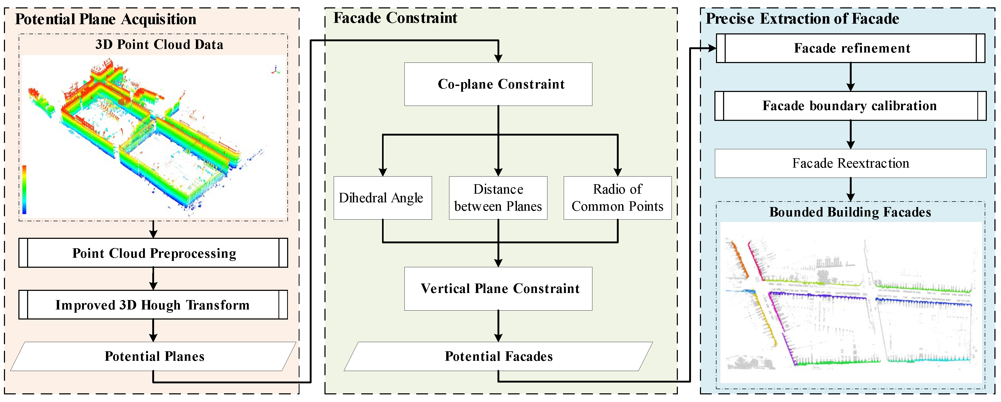
2.1. Building Facade Extraction
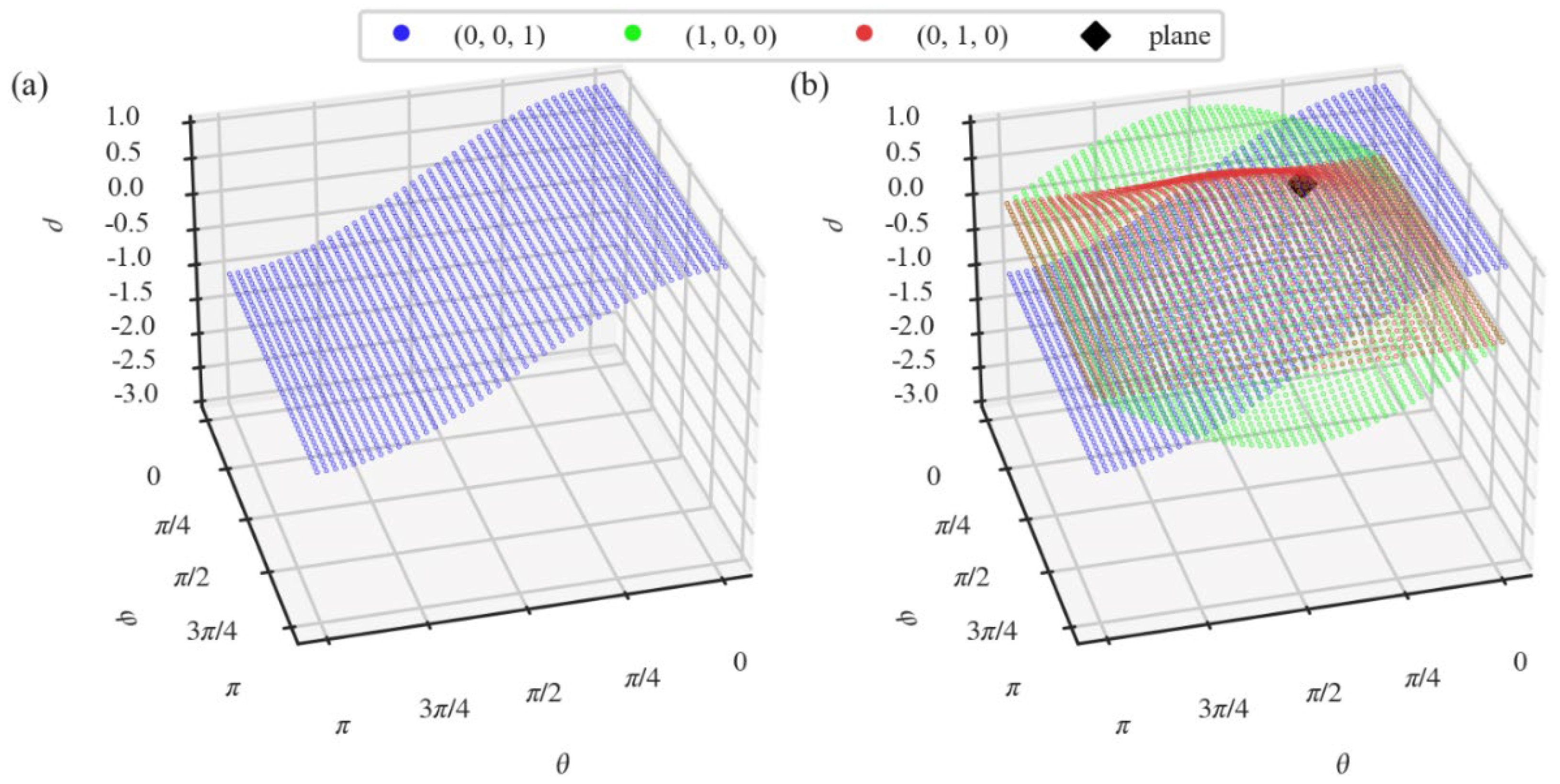
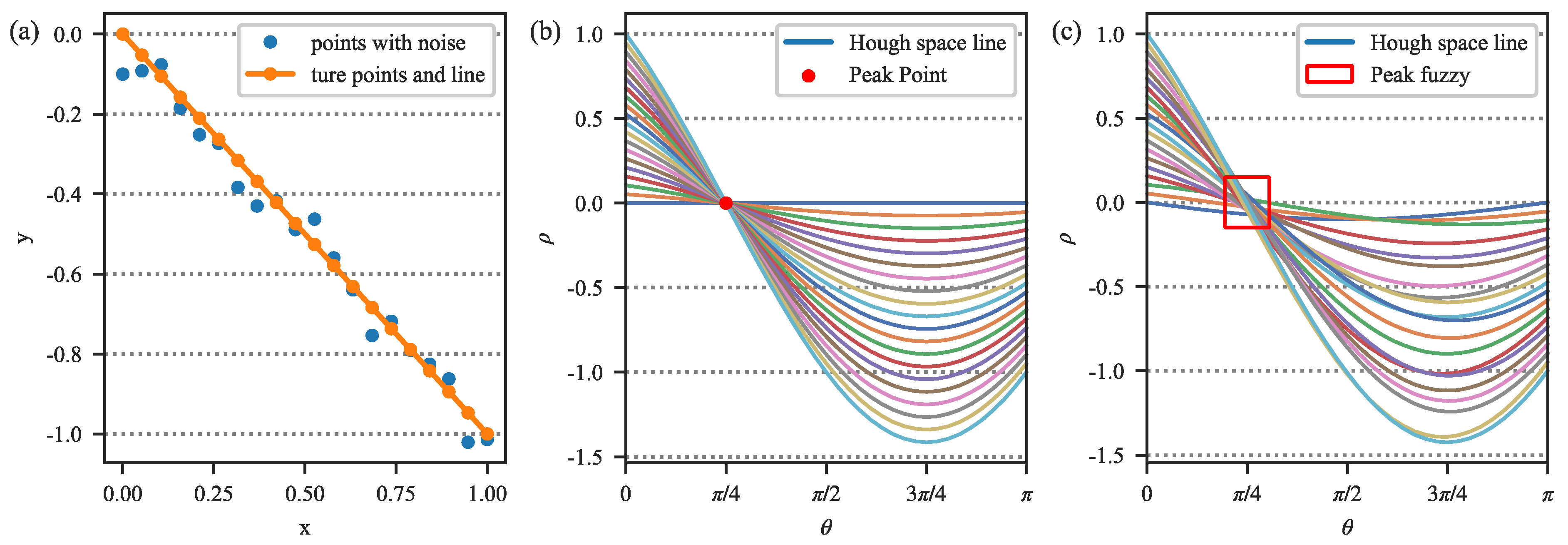
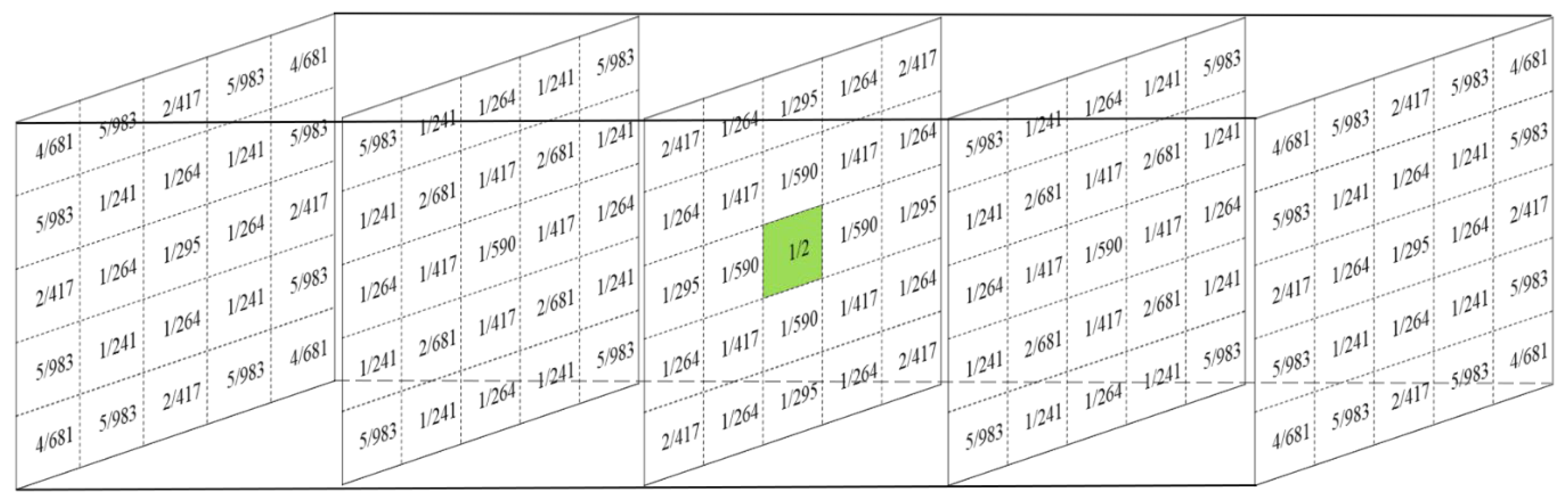
2.1.1. Improved 3D HT for Potential Plane Acquisition
2.1.2. Facade Constraints
2.1.3. Precise Extraction of Facade
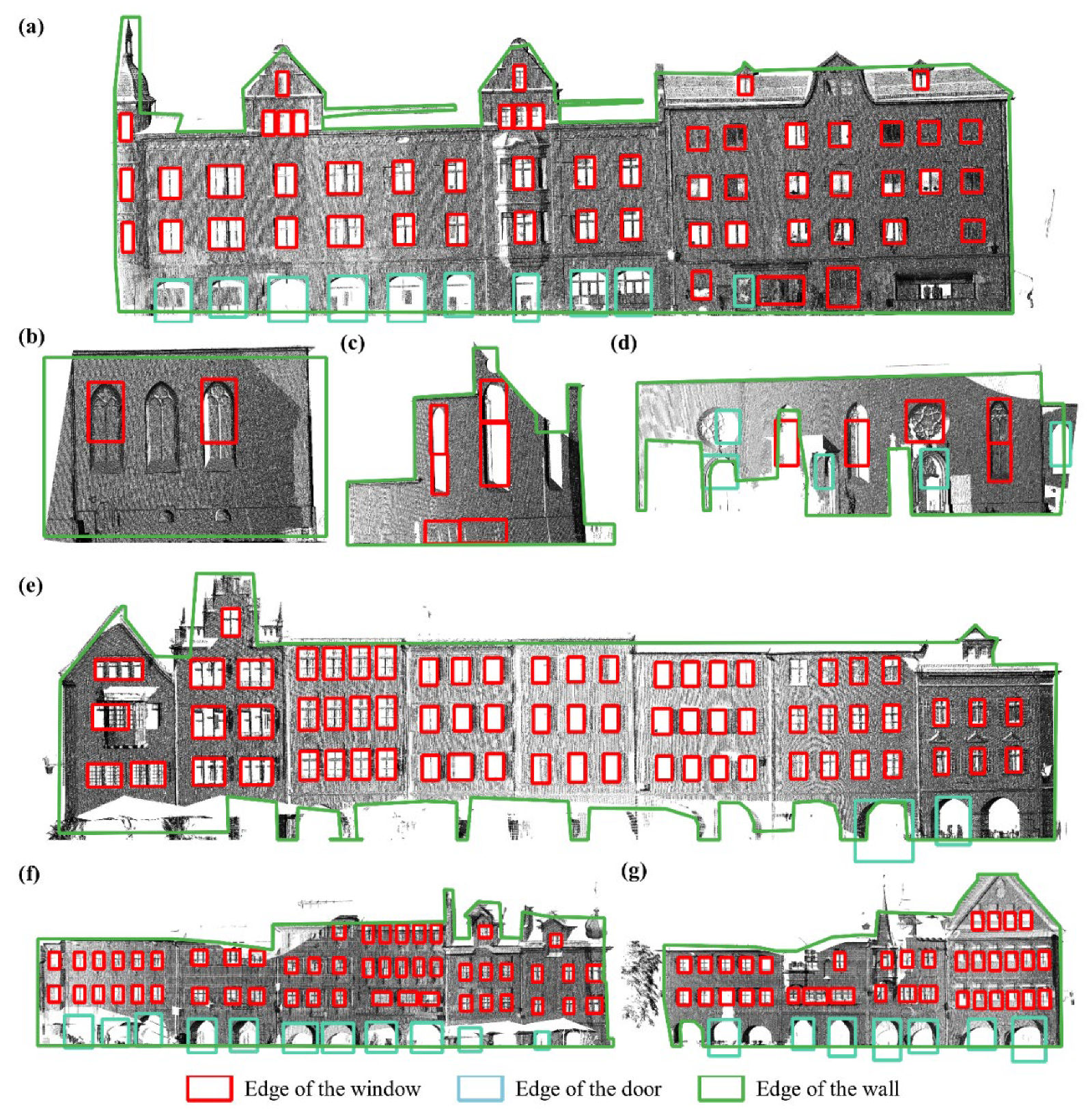
2.2. Building Facade Map Extraction
3. Experiments and Results
3.1. Results of the IQmulus & TerraMobilita Contest Dataset
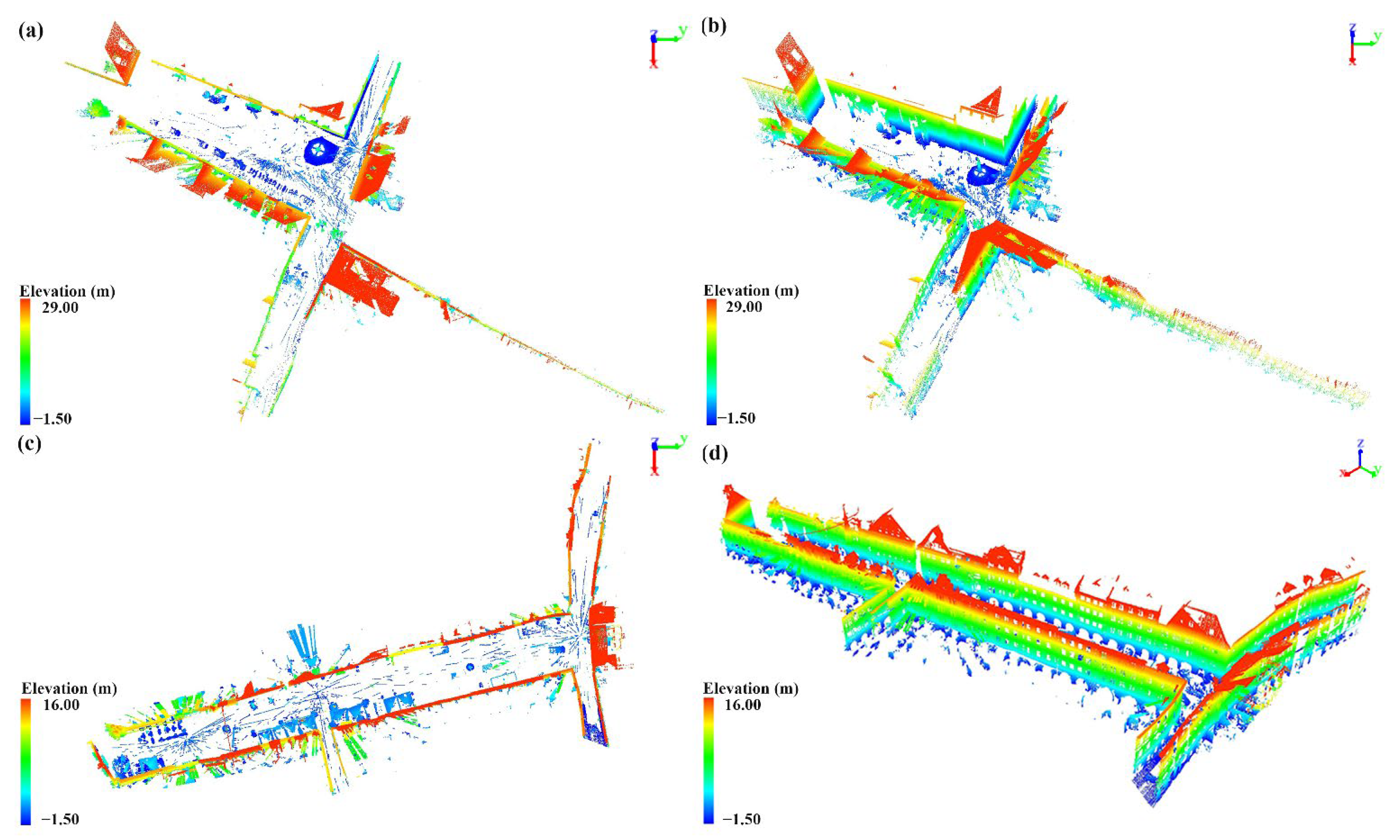
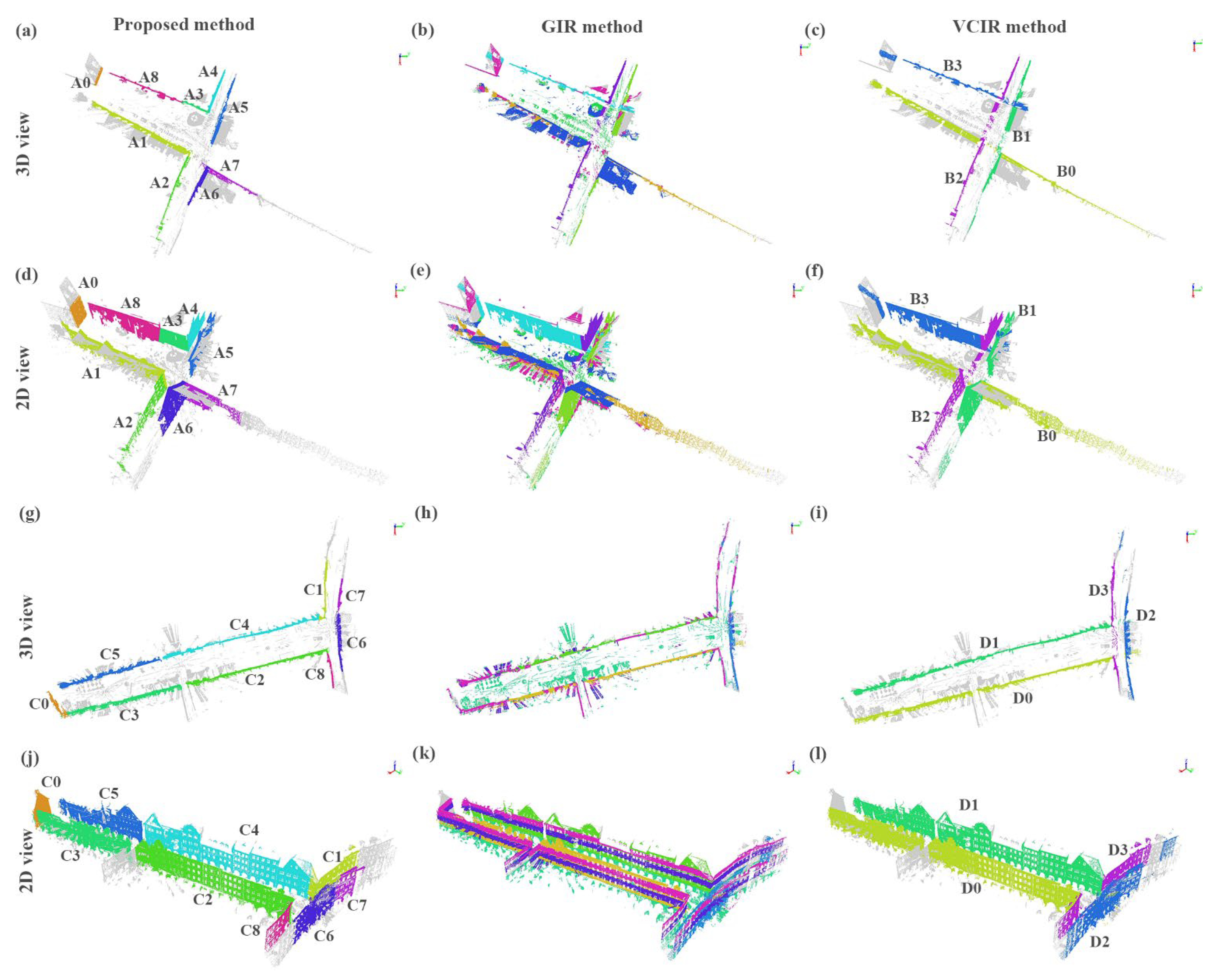
3.2. Results of the Semantic3D.Net Benchmark Dataset
4. Discussion
5. Conclusions
Author Contributions
Funding
Acknowledgments
Conflicts of Interest
References
- Wang, Y.; Ma, Y.; Zhu, A.; Zhao, H.; Liao, L. Accurate Facade Feature Extraction Method for Buildings from Three-Dimensional Point Cloud Data Considering Structural Information. ISPRS J. Photogramm. Remote Sens. 2018, 139, 146–153. [Google Scholar] [CrossRef]
- Liang, X.; Fu, Z.; Sun, C.; Hu, Y. MHIBS-Net: Multiscale Hierarchical Network for Indoor Building Structure Point Clouds Semantic Segmentation. Int. J. Appl. Earth Obs. Geoinf. 2021, 102, 102449. [Google Scholar] [CrossRef]
- Wang, Q.; Kim, M.-K. Applications of 3D Point Cloud Data in the Construction Industry: A Fifteen-Year Review from 2004 to 2018. Adv. Eng. Inform. 2019, 39, 306–319. [Google Scholar] [CrossRef]
- Malihi, S.; Valadan Zoej, M.J.; Hahn, M. Large-Scale Accurate Reconstruction of Buildings Employing Point Clouds Generated from UAV Imagery. Remote Sens. 2018, 10, 1148. [Google Scholar] [CrossRef] [Green Version]
- Teboul, O.; Simon, L.; Koutsourakis, P.; Paragios, N. Segmentation of building facades using procedural shape priors. In Proceedings of the 2010 IEEE Computer Society Conference on Computer Vision and Pattern Recognition, San Francisco, CA, USA, 13–18 June 2010; pp. 3105–3112. [Google Scholar]
- Xie, L.; Zhu, Q.; Hu, H.; Wu, B.; Li, Y.; Zhang, Y.; Zhong, R. Hierarchical Regularization of Building Boundaries in Noisy Aerial Laser Scanning and Photogrammetric Point Clouds. Remote Sens. 2018, 10, 1996. [Google Scholar] [CrossRef] [Green Version]
- Xie, L.; Hu, H.; Zhu, Q.; Li, X.; Tang, S.; Li, Y.; Guo, R.; Zhang, Y.; Wang, W. Combined Rule-Based and Hypothesis-Based Method for Building Model Reconstruction from Photogrammetric Point Clouds. Remote Sens. 2021, 13, 1107. [Google Scholar] [CrossRef]
- Zhou, M.; Ma, L.; Li, Y.; Li, J. Extraction of building windows from mobile laser scanning point clouds. In Proceedings of the IGARSS 2018—2018 IEEE International Geoscience and Remote Sensing Symposium, Valencia, Spain, 22–27 July 2018; pp. 4304–4307. [Google Scholar]
- Hao, W.; Wang, Y.; Liang, W. Slice-Based Building Facade Reconstruction from 3D Point Clouds. Int. J. Remote Sens. 2018, 39, 6587–6606. [Google Scholar] [CrossRef]
- Li, J.; Xiong, B.; Biljecki, F.; Schrotter, G. A Sliding Window Method for Detecting Corners of Openings from Terrestrial LiDAr Data. Int. Arch. Photogramm. Remote Sens. Spat. Inf. Sci. 2018, 42, 97–103. [Google Scholar] [CrossRef] [Green Version]
- Zolanvari, S.I.; Laefer, D.F. Slicing Method for Curved Facade and Window Extraction from Point Clouds. ISPRS J. Photogramm. Remote Sens. 2016, 119, 334–346. [Google Scholar] [CrossRef]
- Biosca, J.M.; Lerma, J.L. Unsupervised Robust Planar Segmentation of Terrestrial Laser Scanner Point Clouds Based on Fuzzy Clustering Methods. ISPRS J. Photogramm. Remote Sens. 2008, 63, 84–98. [Google Scholar] [CrossRef]
- Dong, Z.; Yang, B.; Hu, P.; Scherer, S. An Efficient Global Energy Optimization Approach for Robust 3D Plane Segmentation of Point Clouds. ISPRS J. Photogramm. Remote Sens. 2018, 137, 112–133. [Google Scholar] [CrossRef]
- Maas, H.-G.; Vosselman, G. Two Algorithms for Extracting Building Models from Raw Laser Altimetry Data. ISPRS J. Photogramm. Remote Sens. 1999, 54, 153–163. [Google Scholar] [CrossRef]
- Limberger, F.A.; Oliveira, M.M. Real-Time Detection of Planar Regions in Unorganized Point Clouds. Pattern Recognit. 2015, 48, 2043–2053. [Google Scholar] [CrossRef] [Green Version]
- Xu, Y.; Ye, Z.; Huang, R.; Hoegner, L.; Stilla, U. Robust Segmentation and Localization of Structural Planes from Photogrammetric Point Clouds in Construction Sites. Autom. Constr. 2020, 117, 103206. [Google Scholar] [CrossRef]
- Adam, A.; Chatzilari, E.; Nikolopoulos, S.; Kompatsiaris, I. H-RANSAC: A Hybrid Point Cloud Segmentation Combining 2D and 3D Data. ISPRS Ann. Photogramm. Remote Sens. Spat. Inf. Sci. 2018, 4, 1–8. [Google Scholar] [CrossRef] [Green Version]
- Ebrahimi, A.; Czarnuch, S. Automatic Super-Surface Removal in Complex 3D Indoor Environments Using Iterative Region-Based RANSAC. Sensors 2021, 21, 3724. [Google Scholar] [CrossRef]
- Qi, C.R.; Su, H.; Mo, K.; Guibas, L.J. PointNet: Deep learning on point sets for 3D classification and segmentation. In Proceedings of the IEEE Conference on Computer Vision and Pattern Recognition (CVPR 2017), Honolulu, HI, USA, 21–26 July 2017; pp. 77–85. [Google Scholar]
- Lin, H.; Wu, S.; Chen, Y.; Li, W.; Luo, Z.; Guo, Y.; Wang, C.; Li, J. Semantic Segmentation of 3D Indoor LiDAR Point Clouds through Feature Pyramid Architecture Search. ISPRS J. Photogramm. Remote Sens. 2021, 177, 279–290. [Google Scholar] [CrossRef]
- Chen, Y.; Wu, R.; Yang, C.; Lin, Y. Urban Vegetation Segmentation Using Terrestrial LiDAR Point Clouds Based on Point Non-Local Means Network. Int. J. Appl. Earth Obs. Geoinf. 2021, 105, 102580. [Google Scholar] [CrossRef]
- Haghighatgou, N.; Daniel, S.; Badard, T. A Method for Automatic Identification of Openings in Buildings Facades Based on Mobile LiDAR Point Clouds for Assessing Impacts of Floodings. Int. J. Appl. Earth Obs. Geoinf. 2022, 108, 102757. [Google Scholar] [CrossRef]
- Alshawabkeh, Y. Linear Feature Extraction from Point Cloud Using Color Information. Herit. Sci. 2020, 8, 28. [Google Scholar] [CrossRef]
- Díaz-Vilariño, L.; Khoshelham, K.; Martínez-Sánchez, J.; Arias, P. 3D Modeling of Building Indoor Spaces and Closed Doors from Imagery and Point Clouds. Sensors 2015, 15, 3491–3512. [Google Scholar] [CrossRef] [Green Version]
- Duda, R.O.; Hart, P.E. Use of the Hough Transformation to Detect Lines and Curves in Pictures. Commun. ACM 1972, 15, 11–15. [Google Scholar] [CrossRef]
- Borrmann, D.; Elseberg, J.; Lingemann, K.; Nüchter, A. The 3D Hough Transform for Plane Detection in Point Clouds: A Review and a New Accumulator Design. 3D Res. 2011, 2, 3. [Google Scholar] [CrossRef]
- Li, N.; Ma, Y.; Yang, Y.; Gao, S. An Improved Method of Lee Refined Polarized Filter. Sci. Surv. Mapp. 2011, 36, 144–145+138. [Google Scholar]
- Campello, R.J.G.B.; Moulavi, D.; Sander, J. Density-based clustering based on hierarchical density estimates. In Advances in Knowledge Discovery and Data Mining; Springer: Berlin/Heidelberg, Germany, 2013; pp. 160–172. [Google Scholar]
- Girshick, R.; Donahue, J.; Darrell, T.; Malik, J. Rich feature hierarchies for accurate object detection and semantic segmentation. In Proceedings of the IEEE Conference on Computer Vision and Pattern Recognition, San Juan, PR, USA, 17–19 June 1997; pp. 580–587. [Google Scholar]
- He, K.; Zhang, X.; Ren, S.; Sun, J. Spatial Pyramid Pooling in Deep Convolutional Networks for Visual Recognition. IEEE Trans. Pattern Anal. Mach. Intell. 2015, 37, 1904–1916. [Google Scholar] [CrossRef] [Green Version]
- Liu, W.; Anguelov, D.; Erhan, D.; Szegedy, C.; Reed, S.; Fu, C.-Y.; Berg, A.C. SSD: Single shot MultiBox detector. In Computer Vision—ECCV 2016; Lecture Notes in Computer Science; Springer: Cham, Switzerland, 2016; Volume 9905, pp. 21–37. [Google Scholar] [CrossRef] [Green Version]
- Redmon, J.; Divvala, S.; Girshick, R.; Farhadi, A. You only look once: Unified, real-time object detection. arXiv 2016, arXiv:1506.02640. [Google Scholar]
- Ren, S.; He, K.; Girshick, R.; Sun, J. Faster R-CNN: Towards real-time object detection with region proposal networks. arXiv 2016, arXiv:1506.01497. [Google Scholar] [CrossRef] [Green Version]
- Ma, L.; Liu, Y.; Zhang, X.; Ye, Y.; Yin, G.; Johnson, B.A. Deep Learning in Remote Sensing Applications: A Meta-Analysis and Review. ISPRS J. Photogramm. Remote Sens. 2019, 152, 166–177. [Google Scholar] [CrossRef]
- Esri Automation of Map Generalization: The Cutting-Edge Technology. 1996. White Paper. Redlands, ESRI Inc. Available online: http://downloads.esri.com/support/whitepapers/ao_/mapgen.pdf (accessed on 12 June 2022).
- Vallet, B.; Brédif, M.; Serna, A.; Marcotegui, B.; Paparoditis, N. TerraMobilita/IQmulus Urban Point Cloud Analysis Benchmark. Comput. Graph. 2015, 49, 126–133. [Google Scholar] [CrossRef] [Green Version]
- Hackel, T.; Savinov, N.; Ladicky, L.; Wegner, J.D.; Schindler, K.; Pollefeys, M. Semantic3d. Net: A New Large-Scale Point Cloud Classification Benchmark. ISPRS Ann. Photogramm. Remote Sens. Spat. Inf. Sci. 2017, 41, 91–98. [Google Scholar] [CrossRef] [Green Version]
- Smith, L.N. Cyclical learning rates for training neural networks. In Proceedings of the 2017 IEEE Winter Conference on Applications of Computer Vision (WACV), Santa Rosa, CA, USA, 24–31 March 2017; pp. 464–472. [Google Scholar]
- Qi, C.R.; Yi, L.; Su, H.; Guibas, L.J. PointNet++: Deep hierarchical feature learning on point sets in a metric space. In Advances in Neural Information Processing Systems 30 (NeurIPS 2017); Guyon, I., Luxburg, U.V., Bengio, S., Wallach, H., Fergus, R., Vishwanathan, S., Garnett, R., Eds.; Neural Information Processing Systems (NIPS): La Jolla, CA, USA, 2017; Volume 30. [Google Scholar]


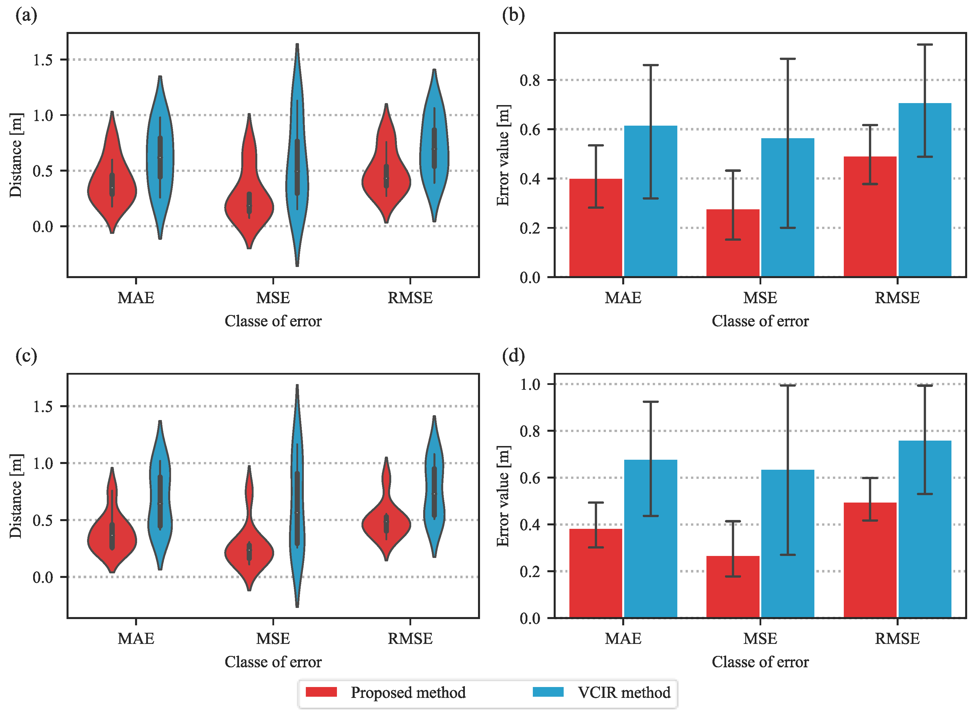
| Method | Number of Extract Facade | MAE | MSE | RMSE |
|---|---|---|---|---|
| Proposed method | I0 | 0.427 | 0.253 | 0.503 |
| I1 | 0.216 | 0.102 | 0.319 | |
| I2 | 0.186 | 0.085 | 0.291 | |
| I3 | 0.241 | 0.109 | 0.330 | |
| I4 | 0.321 | 0.172 | 0.415 | |
| I5 | 0.386 | 0.247 | 0.497 | |
| I6 | 0.597 | 0.426 | 0.653 | |
| I7 | 0.502 | 0.413 | 0.643 | |
| I8 | 0.244 | 0.097 | 0.312 | |
| I9 | 0.332 | 0.190 | 0.435 | |
| I10 | 0.761 | 0.696 | 0.835 | |
| I11 | 0.446 | 0.302 | 0.550 | |
| I12 | 0.585 | 0.425 | 0.652 | |
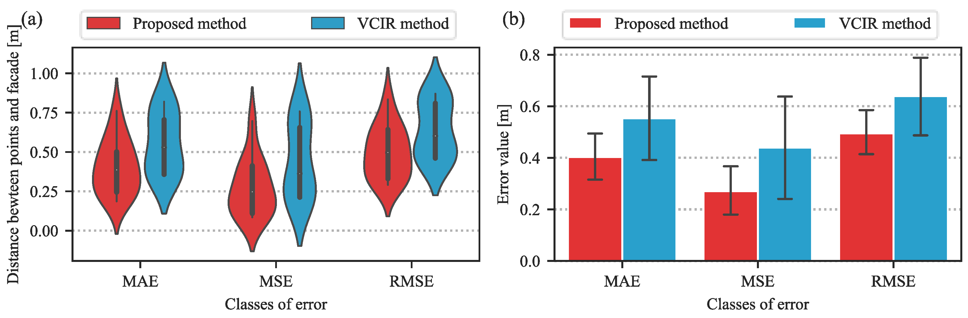
| MEFE | 0.403 | 0.271 | 0.495 | |
| OFE | 0.314 | 0.194 | 0.440 | |
| VCIR method | II0 | 0.820 | 0.758 | 0.871 |
| II1 | 0.357 | 0.208 | 0.456 | |
| II2 | 0.357 | 0.212 | 0.461 | |
| II3 | 0.529 | 0.363 | 0.602 | |
| II4 | 0.705 | 0.656 | 0.810 | |
| MEFE | 0.554 | 0.439 | 0.640 | |
| OFE | 0.500 | 0.403 | 0.634 |
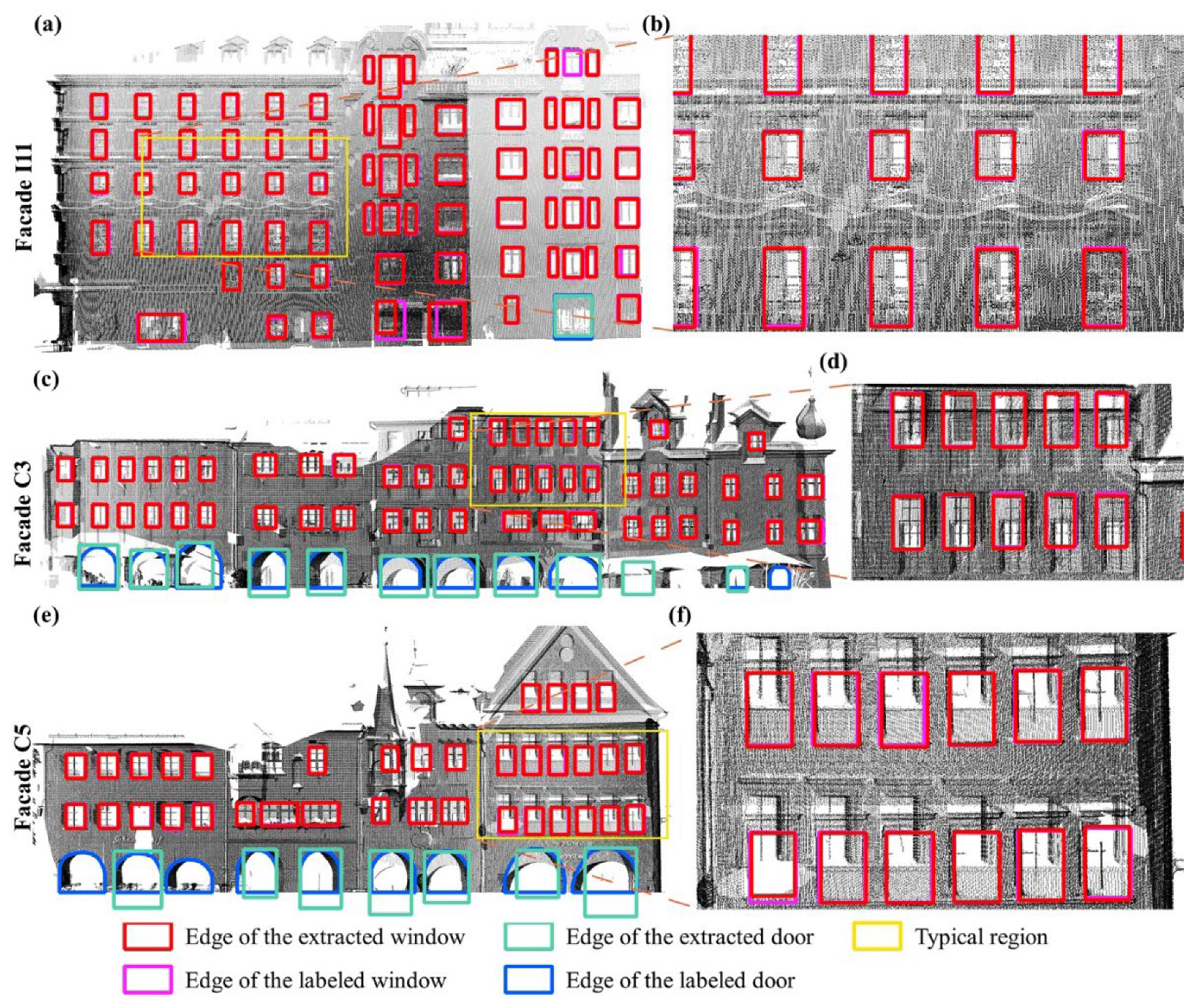
| ID of the Facade | MinIoU: 50% | MinIoU: 85% | ||||||
|---|---|---|---|---|---|---|---|---|
| Precision | Recall | F1 Score | AP | Precision | Recall | F1 Score | AP | |
| I0 | 1.000 | 1.000 | 1.000 | 1.000 | 0.933 | 0.933 | 0.933 | 0.871 |
| I1 | 1.000 | 1.000 | 1.000 | 1.000 | 0.947 | 0.947 | 0.947 | 0.898 |
| I2 | 1.000 | 0.974 | 0.987 | 0.974 | 0.921 | 0.897 | 0.909 | 0.827 |
| I3 | 0.986 | 0.959 | 0.972 | 0.952 | 0.845 | 0.822 | 0.833 | 0.719 |
| I4 | 1.000 | 1.000 | 1.000 | 1.000 | 1.000 | 1.000 | 1.000 | 1.000 |
| I5 | 0.986 | 0.986 | 0.986 | 0.986 | 0.890 | 0.890 | 0.890 | 0.827 |
| I6 | 0.912 | 0.981 | 0.945 | 0.945 | 0.842 | 0.906 | 0.873 | 0.805 |
| I7 | 1.000 | 0.976 | 0.988 | 0.976 | 0.901 | 0.880 | 0.890 | 0.793 |
| I8 | 0.964 | 1.000 | 0.981 | 0.964 | 0.891 | 0.925 | 0.907 | 0.839 |
| I9 | 1.000 | 1.000 | 1.000 | 1.000 | 0.949 | 0.949 | 0.949 | 0.900 |
| I10 | 1.000 | 0.938 | 0.968 | 0.938 | 0.959 | 0.899 | 0.928 | 0.862 |
| I11 | 0.947 | 0.992 | 0.969 | 0.969 | 0.848 | 0.889 | 0.868 | 0.784 |
| I12 | 1.000 | 0.987 | 0.994 | 0.987 | 0.779 | 0.769 | 0.774 | 0.621 |
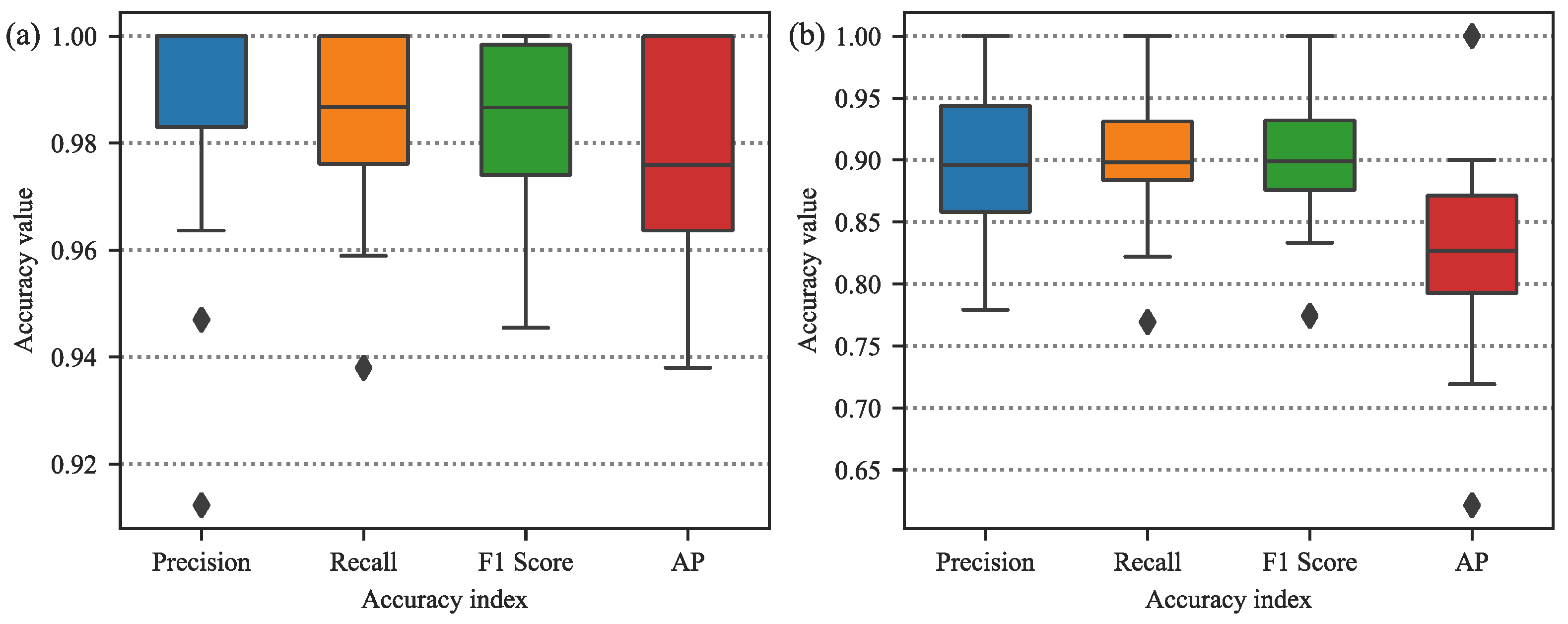
| Mean value of each facade | 0.984 | 0.984 | 0.984 | 0.976 | 0.901 | 0.900 | 0.900 | 0.827 |
| All facade | 0.982 | 0.977 | 0.979 | - | 0.887 | 0.882 | 0.884 | - |
| Scene Name | Method | Number of Extracted Facade | MAE | MSE | RMSE |
|---|---|---|---|---|---|
| domfountain | Proposed method | A0 | 0.204 | 0.074 | 0.272 |
| A1 | 0.287 | 0.151 | 0.389 | ||
| A2 | 0.598 | 0.572 | 0.756 | ||
| A3 | 0.177 | 0.094 | 0.306 | ||
| A4 | 0.346 | 0.185 | 0.430 | ||
| A5 | 0.460 | 0.281 | 0.531 | ||
| A6 | 0.299 | 0.131 | 0.363 | ||
| A7 | 0.460 | 0.289 | 0.538 | ||
| A8 | 0.793 | 0.736 | 0.858 | ||
| MEFE | 0.403 | 0.279 | 0.494 | ||
| OFE | 0.335 | 0.222 | 0.471 | ||
| VCIR method | B0 | 0.979 | 1.129 | 1.063 | |
| B1 | 0.257 | 0.152 | 0.390 | ||
| B2 | 0.505 | 0.344 | 0.587 | ||
| B3 | 0.731 | 0.643 | 0.802 | ||
| MEFE | 0.618 | 0.567 | 0.710 | ||
| OFE | 0.494 | 0.418 | 0.647 | ||
| marketplacefeldkirch | Proposed method | C0 | 0.462 | 0.307 | 0.554 |
| C1 | 0.757 | 0.746 | 0.864 | ||
| C2 | 0.243 | 0.144 | 0.379 | ||
| C3 | 0.417 | 0.246 | 0.496 | ||
| C4 | 0.366 | 0.236 | 0.486 | ||
| C5 | 0.240 | 0.162 | 0.403 | ||
| C6 | 0.267 | 0.195 | 0.442 | ||
| C7 | 0.259 | 0.110 | 0.331 | ||
| C8 | 0.460 | 0.279 | 0.528 | ||
| MEFE | 0.386 | 0.269 | 0.498 | ||
| OFE | 0.296 | 0.198 | 0.445 | ||
| VCIR method | D0 | 0.457 | 0.306 | 0.553 | |
| D1 | 0.416 | 0.258 | 0.508 | ||
| D2 | 1.019 | 1.165 | 1.079 | ||
| D3 | 0.830 | 0.823 | 0.907 | ||
| MEFE | 0.681 | 0.638 | 0.762 | ||
| OFE | 0.464 | 0.385 | 0.621 |
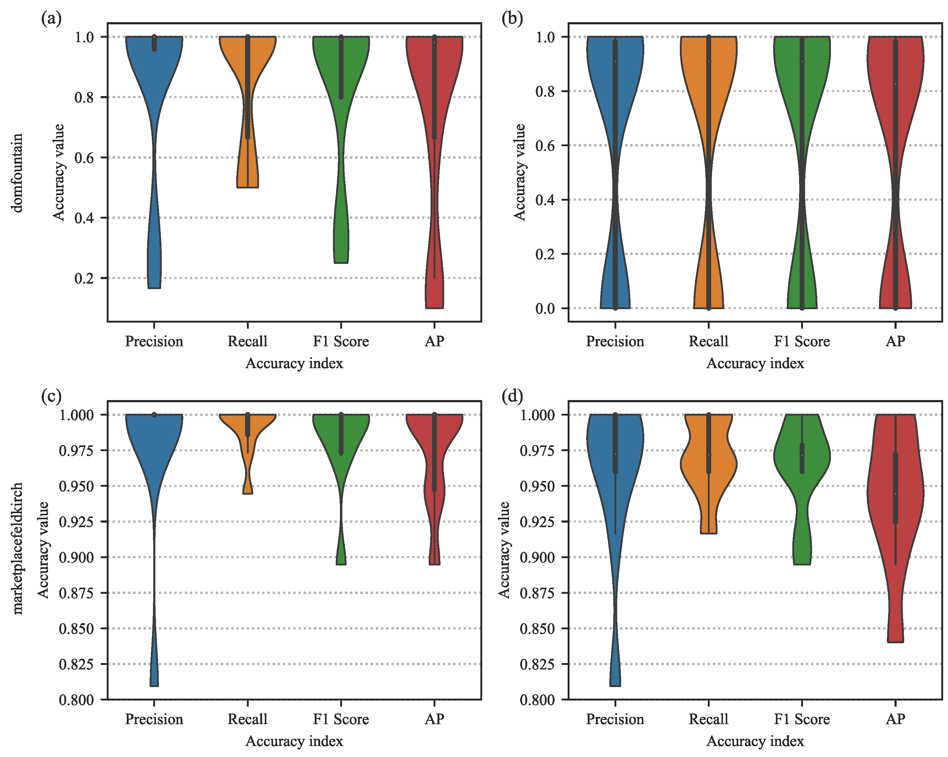
| Scene Name | ID of the Facade | Min IoU: 50% | Min IoU: 85% | ||||||
|---|---|---|---|---|---|---|---|---|---|
| Precision | Recall | F1 Score | AP | Precision | Recall | F1 Score | AP | ||
| domfountain | A0 | 1.000 | 1.000 | 1.000 | 1.000 | 0.909 | 0.909 | 0.909 | 0.826 |
| A1 | 0.981 | 1.000 | 0.991 | 0.981 | 0.981 | 1.000 | 0.991 | 0.981 | |
| A2 | 0.958 | 0.958 | 0.958 | 0.918 | 0.875 | 0.875 | 0.875 | 0.766 | |
| A3 | 1.000 | 0.667 | 0.800 | 0.667 | 0.000 | 0.000 | 0.000 | 0.000 | |
| A4 | 0.167 | 0.500 | 0.250 | 0.100 | 0.000 | 0.000 | 0.000 | 0.000 | |
| A5 | 1.000 | 1.000 | 1.000 | 1.000 | 1.000 | 1.000 | 1.000 | 1.000 | |
| A6 | 1.000 | 1.000 | 1.000 | 1.000 | 1.000 | 1.000 | 1.000 | 1.000 | |
| A7 | 1.000 | 1.000 | 1.000 | 1.000 | 0.952 | 0.952 | 0.952 | 0.907 | |
| A8 | 0.333 | 0.500 | 0.400 | 0.200 | 0.000 | 0.000 | 0.000 | 0.000 | |
| Mean value of each facade | 0.888 | 0.891 | 0.875 | 0.833 | 0.715 | 0.717 | 0.716 | 0.685 | |
| All facade | 0.936 | 0.970 | 0.953 | - | 0.884 | 0.916 | 0.900 | - | |
| marketplacefeldkirch | C0 | 1.000 | 1.000 | 1.000 | 1.000 | 1.000 | 1.000 | 1.000 | 1.000 |
| C1 | 0.810 | 1.000 | 0.895 | 0.895 | 0.810 | 1.000 | 0.895 | 0.895 | |
| C2 | 1.000 | 0.986 | 0.993 | 0.986 | 0.986 | 0.972 | 0.979 | 0.958 | |
| C3 | 1.000 | 1.000 | 1.000 | 1.000 | 0.962 | 0.962 | 0.962 | 0.925 | |
| C4 | 0.973 | 0.973 | 0.973 | 0.947 | 0.960 | 0.960 | 0.960 | 0.934 | |
| C5 | 1.000 | 1.000 | 1.000 | 1.000 | 0.972 | 0.972 | 0.972 | 0.972 | |
| C6 | 1.000 | 0.944 | 0.971 | 0.944 | 1.000 | 0.944 | 0.971 | 0.944 | |
| C7 | 1.000 | 1.000 | 1.000 | 1.000 | 1.000 | 1.000 | 1.000 | 1.000 | |
| C8 | 1.000 | 1.000 | 1.000 | 1.000 | 0.917 | 0.917 | 0.917 | 0.840 | |
| Mean value of each facade | 0.976 | 0.989 | 0.981 | 0.975 | 0.956 | 0.970 | 0.962 | 0.941 | |
| All facade | 0.981 | 0.984 | 0.983 | - | 0.962 | 0.965 | 0.964 | - | |
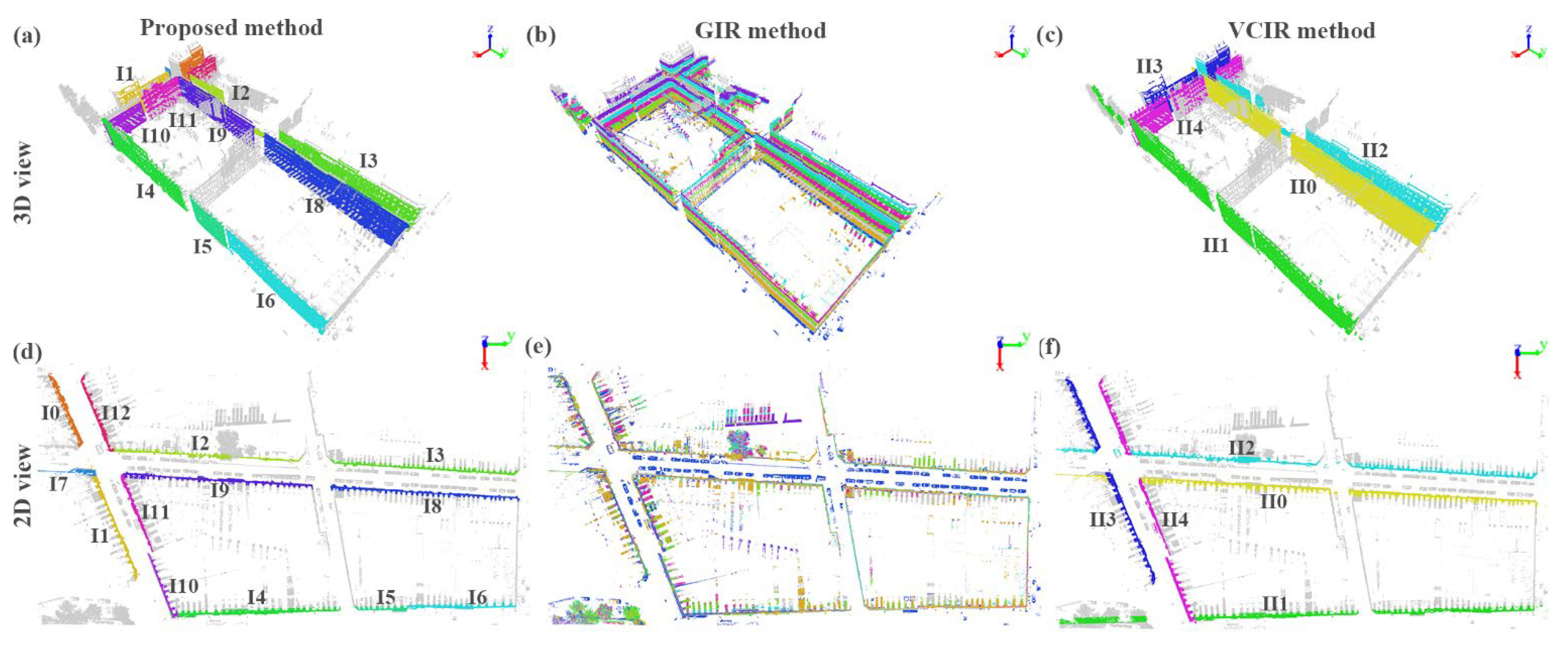
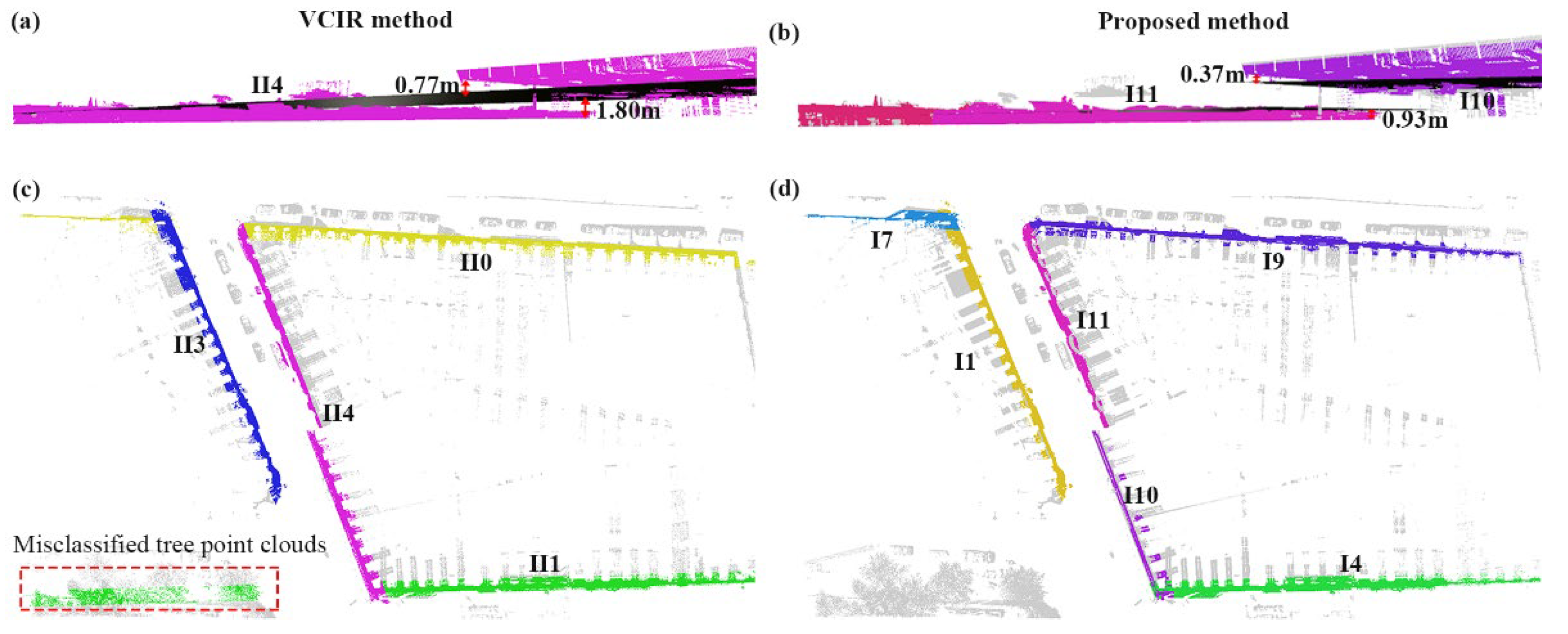
| Results by VCIR Method | Results by Proposed Method |
|---|---|
| II0 | I7, I8, I9 |
| II1 | I4, I5, I6 |
| II2 | I2, I3 |
| II3 | I0, I1 |
| II4 | I10, I11, I12 |
Publisher’s Note: MDPI stays neutral with regard to jurisdictional claims in published maps and institutional affiliations. |
© 2022 by the authors. Licensee MDPI, Basel, Switzerland. This article is an open access article distributed under the terms and conditions of the Creative Commons Attribution (CC BY) license (https://creativecommons.org/licenses/by/4.0/).
Share and Cite
Yu, B.; Hu, J.; Dong, X.; Dai, K.; Xiao, D.; Zhang, B.; Wu, T.; Hu, Y.; Wang, B. A Robust Automatic Method to Extract Building Facade Maps from 3D Point Cloud Data. Remote Sens. 2022, 14, 3848. https://doi.org/10.3390/rs14163848
Yu B, Hu J, Dong X, Dai K, Xiao D, Zhang B, Wu T, Hu Y, Wang B. A Robust Automatic Method to Extract Building Facade Maps from 3D Point Cloud Data. Remote Sensing. 2022; 14(16):3848. https://doi.org/10.3390/rs14163848
Chicago/Turabian StyleYu, Bing, Jinlong Hu, Xiujun Dong, Keren Dai, Dongsheng Xiao, Bo Zhang, Tao Wu, Yunliang Hu, and Bing Wang. 2022. "A Robust Automatic Method to Extract Building Facade Maps from 3D Point Cloud Data" Remote Sensing 14, no. 16: 3848. https://doi.org/10.3390/rs14163848