Article

Peatland Plant Spectral Response as a Proxy for Peat Health, Analysis Using Low-Cost Hyperspectral Imaging Techniques

1
Department of Electronic and Electrical Engineering, University of Sheffield, Sheffield S1 4DE, UK
2
Department of Geography, University of Sheffield, Sheffield S10 2TN, UK
*
Author to whom correspondence should be addressed.
Remote Sens. 2022, 14(16), 3846; https://doi.org/10.3390/rs14163846
Submission received: 23 June 2022 / Revised: 1 August 2022 / Accepted: 5 August 2022 / Published: 9 August 2022
(This article belongs to the Special Issue Application of Remote Sensing for Monitoring of Peatlands)

Abstract

:
Peatland habitats represent key environmental resources that are a critical component in climate change mitigation strategies. However, many of these environmental settings are facing significant levels of erosion and degradation which, over time, will result in the loss of these key environments. Traditional monitoring techniques for these settings require invasive methods, disrupting the natural environment and potentially leading to further losses if incorrectly administered. In this article, we provide a non-invasive, cost-effective alternative to peatland health monitoring through the implementation of low-cost hyperspectral imaging techniques. Using common peatland plant species as a proxy for underlying peat health, we monitor the spectral response of Sphagnum plants under varying degrees of water stress to document their spectral response under these conditions. For this research, we utilise a low-cost, semi-portable High-Resolution Hyperspectral Imager capable of resolving mm-scale targets in conjunction with the ultra-low-cost Hyperspectral Smartphone that represents a completely accessible fully field portable instrument allowing for rapid and accurate on-site measurements. Both instruments are shown to provide accurate and robust results, capturing subtle changes in spectral response prior to their appearance within visual datasets enabling the use of mitigation and restoration techniques before the onset of more damaging conditions.

1. Introduction

The continued monitoring and preservation of peatland environments is of significant importance to people, wildlife, and the planet [1,2,3]. Peatlands represent important terrestrial carbon stores [4,5,6,7], and provide habitats for a variety of rare plant and animal species [4,6,8], as well as being natural providers of water regulation and valuable records of our past [1,2]. They play a key role in the global carbon cycle, storing ca. 30% of soil organic carbon, despite only representing ca. 3% of global land surface coverage [7,8,9,10], highlighting their importance for carbon storage and sequestration in a warming world. However, despite these key benefits, many peatland environments are subject to severe levels of erosion and degradation [9,11,12], resulting in a substantial reduction in the quality of the ecosystem services they are capable of providing. This, in turn, can result in these vast carbon stores reverting to carbon sources, releasing carbon back into the atmosphere, and can ultimately lead to the loss of peatland areas [7,11,13,14,15]. Monitoring the overall health of these environments, and the natural processes taking place within them, is, therefore, of significant importance. It allows us to gain a better understanding of these environments and the factors influencing the progression of degradation and erosion in these locations.
Spectral information acquired from above ground vegetation communities has been shown to be an effective means of estimating a variety of factors relating to the health of underlying peat deposits. It has provided valuable insights, from moisture content [10,14,16,17,18], to below-ground carbon stock [13,19], and nitrogen content estimations [20]. These approaches have been shown to provide a non-invasive alternative to conventional fieldwork techniques [14], allowing for larger study locations to be analysed over considerably shorter time scales [18]. Sphagnum moss is a key peatland genus that has been used extensively in this manner due to its specific characteristics that can affect its spectral response and, as such, can be used to estimate below ground peat conditions without the need for coring or other invasive peat sampling methods [16,21,22,23,24]. Generally, the presence of Sphagnum mosses across a peatland area is an indication of good below-ground conditions [16,25]. These mosses thrive in the waterlogged environments of healthy peatland areas, but have been shown to decrease photosynthesis activity and perform more poorly in areas where the below-ground water content is reduced [26,27,28,29,30,31]. These changes in photosynthesis activity result in changes in the spectral response of these mosses, with bleaching occurring as they start to dry out [29,32,33]. By monitoring these variations, it allows for estimates relating to below-ground water table conditions and general peat health to be inferred, in turn, providing a means of long-term, non-destructive monitoring. In this article, we demonstrate that low-cost hyperspectral imaging instruments represent viable alternatives to existing instrumentation and monitoring methods. The Hyperspectral Smartphone, initially described in [34], and updated for handheld applications within [35]; and the Low-Cost High-Resolution Hyperspectral Imager [36], are applied to the field of peatland health monitoring. Sphagnum samples under varying degrees of water stress are analysed under laboratory conditions with the aim of developing a spectral library that can be used to inform non-destructive, in-situ analyses of peatland environments, providing an early warning monitoring system for the onset of poorer conditions in these indispensable natural environments.

2. Materials and Methods

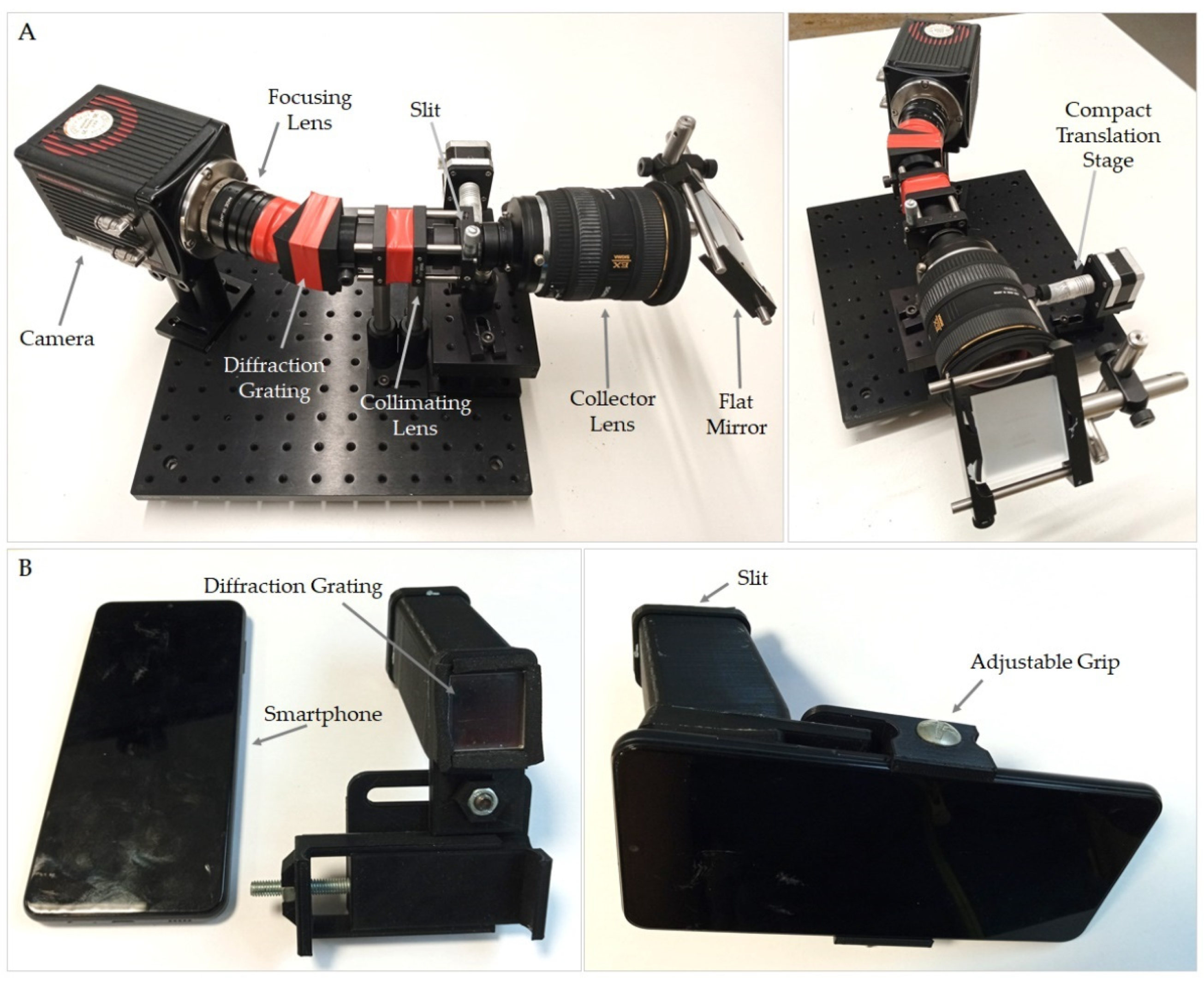
2.1. Instrument Specifications

For this research, two low-cost hyperspectral imaging instruments, previously developed by the authors, were utilised to demonstrate the proficiency, and potential, of these low-cost alternatives to currently available commercial instrumentation. The specific instruments applied to this study (Figure 1) were: the Hyperspectral Smartphone [34,35], an ultra-low-cost, field-portable hyperspectral instrument; and the Low-Cost High-Resolution Hyperspectral Imager [36], a low-cost semi-portable instrument capable of capturing mm-scale targets. Note, the term “ultra-low-cost” is used to describe instrumentation that is significantly cheaper than typical, commercially available options; for example, the Hyperspectral Smartphone costs <£100 to develop, and in contrast, commercial instrumentation typically costs within the region of £30,000 [37]. The High-Resolution instrument costs ca. £11,000 to develop. While this is significantly more expensive than the Hyperspectral Smartphone, it remains considerably cheaper than available commercial options and is, therefore, referred to as “low-cost”. Table 1 shows the settings used for each instrument; a more complete description of these instruments and their precise capabilities can be found in their associated publications, as highlighted above. The exposure time and the spectral range of the Low-Cost High-Resolution instrument can be adjusted by the operator to best fit an intended target. All other settings listed within Table 1 are constrained by the limitations of the individual components of each instrument and are, therefore, not adjustable in this instance.
These two instruments were used in tandem for the duration of this research. The Hyperspectral Smartphone represents an ultra-low-cost, easily accessible instrument that is capable of rapid field deployment with minimal operator training. This instrument is, therefore, particularly convenient for wide-spread data analysis, allowing wide areas to be monitored without significant training and at a fraction of the cost of traditional and commercial approaches. The Low-Cost High-Resolution instrument, however, is a more specialized instrument, with more limited portability. These factors mean this instrumentation is most successfully deployed within a laboratory setting, providing valuable learning that can be successfully and rapidly deployed in the field using the Hyperspectral Smartphone. The High-Resolution instrument is capable of significantly more detailed data capture and can, therefore, be utilised to provide a more in-depth analysis of small samples from specific locations rather than blanket coverage. The combination of these two instruments, therefore, provides an insight into the potential provided by low-cost hyperspectral imaging alternatives, demonstrating that expensive commercial instrumentation is not necessarily required for accurate wide-spread hyperspectral imaging analysis.

2.2. Sample Preparation and Simulated Environmental Conditions

To prevent undue disturbance to peatland areas the Sphagnum plants utilised in this research were obtained as samples, cultivated off-site within a micropropagation facility, rather than removing cuttings directly from the moorland. The moorlands at the focus of this research project, located within the Peak District National Park, have been subject to high levels of erosion and degradation, generally characterised by large expanses of bare peat and networks of erosion gullies [38]. These features have been exacerbated by a variety of factors including drainage, controlled burning, livestock grazing, and pollution from nearby urban areas, resulting in these moorlands being among the most degraded within the United Kingdom [39,40]. However, more recently, restoration projects have been undertaken in this area with the aim of halting the losses associated with peatland erosion and returning the blanket peat to its natural, non-eroded state [39,40,41,42]. Many of these restoration projects involve the reintroduction of cultivated Sphagnum plants to areas of bare peat. These cultivated plants and those obtained for this research project were obtained from the same source and are representative of the Sphagnum plants found across the moorland. A total of 30 Sphagnum samples of ca. 6 cm diameter were used. The Sphagnum species distribution within the samples is shown in Table 2.
The Sphagnum samples were split into three separate groups; a control group that was kept at saturation for the duration of the measurement period, a drought group that received no water inputs, and a rainfall group that received simulated rainfall events based on rainfall datasets obtained from a monitoring station situated on Kinder Scout, a moorland plateau within the Peak District National Park. Table 3 shows the individual groups and their inputs for the duration of the measurement period.
Each sample was housed within an individual container (Figure 2). For the duration of the experiment the samples were kept within a controlled environment chamber (Argus Conviron controlled reach-in chamber) to imitate conditions experienced across the Kinder Scout plateau. The environmental data used here were obtained from the Kinder Scout Community Science Monitoring Station maintained by the Moors for the Future Partnership. Within these datasets records captured from April to September across a 4-year monitoring period, (2016–2019) for temperature and relative humidity; (2014–2017) for rainfall datasets were utilised. The months of April to September were selected to provide environmental conditions representative of the months where Sphagnum plants are most active, removing datasets from winter months where plant growth and productivity are typically significantly reduced. Within the controlled environment chamber the samples were kept within a 24-hour day cycle with 12 h of daylight and 12 h of darkness. During hours of daylight the chamber cycled through a gradual increase in light intensity towards midday, reaching a maximum of 400 μmol m−2 s−1, before steadily decreasing towards dusk. Temperature conditions followed a 24-hour cycle based on the average hourly temperature experienced at the environmental monitoring site (Table 4), representing a gradual increase in temperature towards midday, followed by a steady decrease towards dusk. The average relative humidity for the Kinder Scout location was 90.8%. This was replicated within the controlled environment chamber. Rainfall datasets were used to establish the typical rainfall volume and frequency experienced by in-situ Sphagnum plants. The average monthly rainfall was 104 mm occurring over 15 rain days. This equates to approximately 7 mm rainfall every 3–4 days. This approximation was used to simulate manual rainfall events for Sphagnum plants within the rainfall group for the duration of the study period. Figure 2 shows the samples within the controlled environment chamber.

2.3. Data Collection

For the duration of the study, measurements were taken every three days using both the Hyperspectral Smartphone, and the Low-Cost High-Resolution Hyperspectral Imager. Smartphone datasets were captured at a nadir angle, where the samples were placed directly below the observing instrument. The High-Resolution instrument utilised a flat mirror to achieve an approximate nadir angle without tilting the instrument. Datasets were captured with the Hyperspectral Smartphone using the hand-held method discussed by Davies et al., [35]. Each Sphagnum sample was placed within the in-scene reference card and illuminated using two 20 W light emitting diode (LED) lamps situated at either side of the reference card to minimise the influence of shading/bright spots across the scene (Figure 3). The instrument was translated left to right across the scene at a working distance of ca. 1 m. Spectral calibration was completed using the RGB panel of the reference card, allowing for datasets to be easily and accurately compared without the need for additional data collection.
To capture datasets using the High-Resolution instrument, each sample was positioned, in turn, below the external flat mirror resulting in a working distance of ca. 30 cm. Figure 4 shows the instrumental set-up used during data collection with this device. The samples were illuminated by a 30 W halogen lamp situated above the sample to minimise shading across the scene. This thermal illumination system was used because its spectral response better fitted the wavelength range of this instrument, reducing the potential for noise associated with low signal across longer wavelengths, compared to LED illumination. The use of these different illumination sources is accounted for in post-processing where illumination biases are removed from the datasets and, therefore, do not affect the output measurements of these instruments. The compact translation stage was used to produce the hyperspectral image by translating the collector lens of the instrument across the target sample. Both sets of data were corrected for sensor and illumination biases through the subtraction of dark and white reference frames. After all datasets had been collected the spectral response graphs obtained from both the Hyperspectral Smartphone and the Low-Cost High-Resolution instrument were combined using MATLAB (R2018a) to produce a single, continuous spectrum for each sample group for each measurement day.
To combine these datasets, we utilised the region of spectral overlap between the two devices. The 600 nm response for each instrument was selected as the overlap point and both datasets were then cropped accordingly either side of this value. To mitigate any offsets caused by the separate normalization of the different spectral ranges, the Hyperspectral Smartphone dataset was scaled so the relative intensity at the connecting point was equal to the value of the High-Resolution instrument. The combined dataset was then renormalized, preserving the relative intensity acquired by each instrument (Figure 5). These combined datasets were then utilised for further analysis to produce the figures discussed later within this article.
Sphagnum samples were also photographed with a standard RGB camera, and weighed before being returned to the controlled environment chamber. Care was taken to ensure that each sample spent a minimal amount of time outside the chamber, with samples returned to the chamber promptly after their measurements had been completed. Additionally, to reduce any potential influence of edge effects, sample positions within the chamber were rotated randomly after each measurement phase.

3. Results

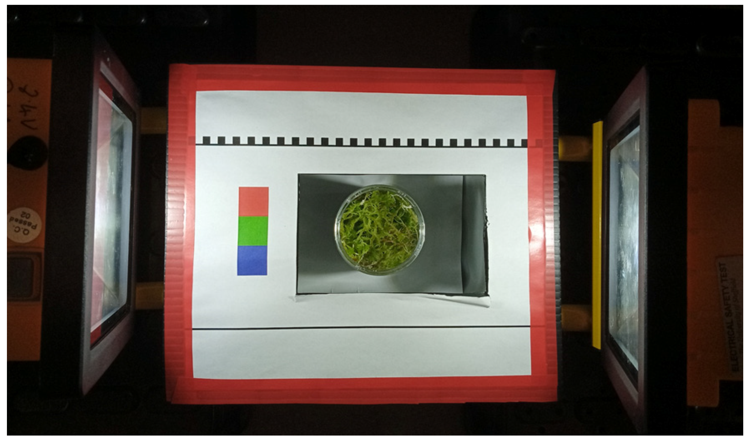
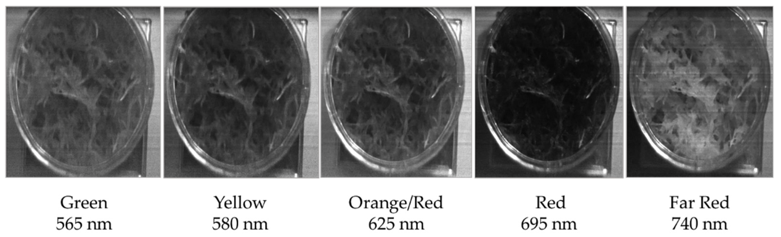
3.1. Spatial Target Identification

Figure 6 shows a spatial and spectral dataset acquired of a Sphagnum sample using the High-Resolution instrument. This example clearly highlights the benefits provided by the high spatial resolution of this instrument. The individual capitula of the Sphagnum plant are clearly recognizable within the images allowing for the spectral response of specific regions of the sample to be determined with significant accuracy. Typically, low-cost hyperspectral imaging instruments are unable to accurately resolve these more intricate features within a more complex target, such as the Sphagnum sample [36]. This is demonstrated in Figure 7 where the spatial datasets of the High-Resolution instrument and the Hyperspectral Smartphone are directly compared. While these instruments have significantly different price points (<£100 vs. ca. £11,000, for the Hyperspectral Smartphone, and the Low-Cost High-Resolution instrument, respectively), making them unfeasible for a true direct comparison, they illustrate the significant difference in spatial clarity of the collected data between two low-cost hyperspectral imaging instruments. This highlights the different applications each instrument is most suited for. For example, the ultra-low-cost Hyperspectral Smartphone provides a rapid and easy detection method enabling datasets to be acquired over numerous locations without the need for extensive operator training. Conversely, the Low-Cost High-Resolution Hyperspectral Imager requires a basic level of expertise and generally represents a more complex instrument. The intricate and detailed datasets acquired using the Low-Cost High-Resolution instrument can, therefore, be used to inform the fully portable, user-friendly Hyperspectral Smartphone, providing valuable learning and intricate target analysis to inform further in-situ investigation.

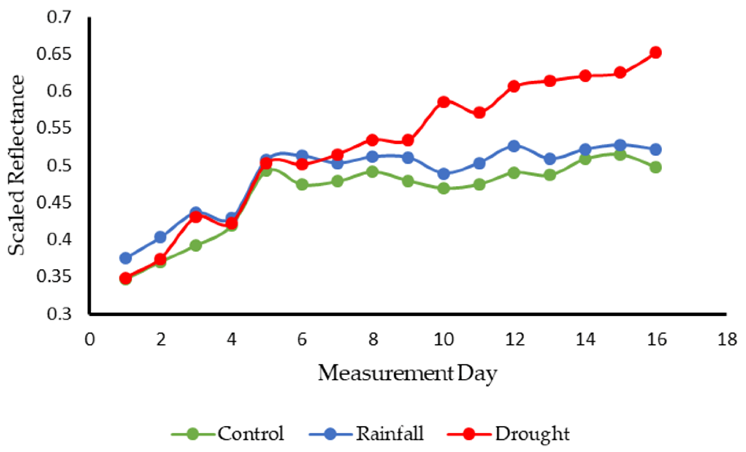
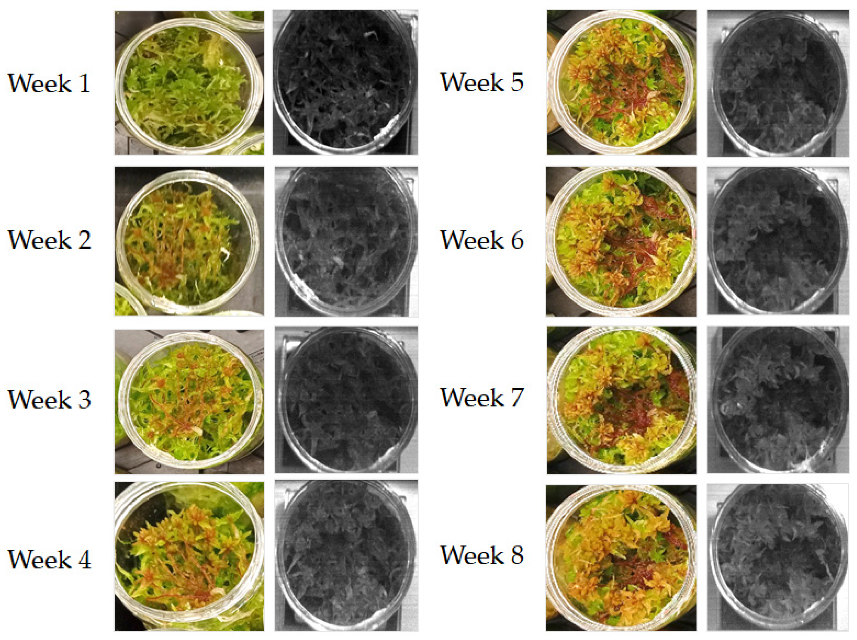
3.2. Change over Time Observations

Hyperspectral imaging datasets were acquired for each Sphagnum plant within each group to determine how the individual samples reacted to their associated water conditions. The results obtained by each instrument were then averaged to provide a single representative response for each set of conditions for each measurement day to enable comparisons to be drawn between different groups and/or different days. Figure 8 shows the averaged spectral change over time observed for each measurement group. In this figure the datasets captured by both instruments were combined to produce an extended dataset that covers the range of 450 nm to 740 nm, providing a comprehensive dataset in which to analyse any spectral changes occurring within the sample groups.
The spectral change over time for each group is clearly visible within these data. All groups can be seen to undergo a period of initial change; however, within the control and rainfall groups, these changes quickly reduce. Conversely, the drought group can be seen to continuously increase in reflectance, resulting in a brighter and flatter spectral response. This is indicative of the bleaching process observed in Sphagnum species undergoing drought and water stress conditions. In the data, the brightness of the drought group’s response can be seen to increase gradually for the duration of the measurement period; however, there are also more subtle changes occurring within this period.
Focusing on the control and rainfall groups, a number of reflectance peaks and absorption features can be identified across their spectral response indicating the presence of a number of pigments within their tissues. The distinct peak present at ca. 550 nm is a key reflectance feature of the Sphagnum species [27,43,44], indicative of healthy conditions. Furthermore, absorption features can also be identified within these spectral curves with a shoulder at ca. 630 nm indicating chlorophyll b absorption and a distinct loss of reflectance at ca. 680 nm highlighting the presence of chlorophyll a [27,43]. These features remain evident within the control and rainfall groups for the duration of the measurements, indicating continued healthy conditions in these groups. However, while these features are initially clear within the drought group, they quickly become less easily discernible as the plants reduce in water content. Looking at Figure 8, subtle differences in the drought group’s spectral response can be observed as early as week two of measurements, with significant differences observed from week three onwards, highlighting rapid changes in spectral response. When these changes are compared with the visual response of the groups, shown in Figure 9 the benefits of hyperspectral imaging techniques become clear.
While clear differences in the spectral response are observable from week three, visual changes in the drought group only begin to show definitive differences from the control and rainfall groups at week five, after which point the drought plants undergo a sudden increase in bleaching. This emphasizes the early warning provided by hyperspectral imaging techniques, providing valuable time for the implementation of mitigation strategies. Furthermore, given the sudden increase in bleaching visually observed in the drought plants it can be inferred that at the point where the Sphagnum plants show these definitive visual signs of water stress the damage may already have taken place. Relying on visual indicators alone, therefore, increases the chances of the plants being lost. This is a serious issue for peatland environments; areas of exposed peat are significantly more likely to be adversely affected by erosion and degradation processes. However, with the early indications observed within the spectral response graphs, there is a much greater opportunity to reduce the impact of poorer below-ground conditions, providing a greater opportunity to revive the affected plants and maintain vegetation coverage.
The differences between the spectral responses of these groups are further illustrated in Figure 10 which shows the averaged spectral change observed at 680 nm for each group. This particular wavelength was selected due to its presence within the region of chlorophyll absorption, providing a more detailed look at spectral change within this region. In this figure, it is clear that all groups underwent a period of initial change. The control and rainfall groups can be seen to undergo a period of increasing reflectance in this region before further increases ceased. From this information it can be inferred that these initial changes were a result of the samples acclimatizing to their new environment. The conditions within the controlled environment chamber were colder than those experienced previously by the Sphagnum samples. The samples, as mentioned above, were obtained from a micropropagation greenhouse with inherently warmer temperature conditions than those experienced by in-situ plants on moorland plateaus. While the samples were given a period of two weeks to acclimatize within the controlled environment prior to the onset of measurements, it is clear that further changes were observed within the first few weeks of measurements. Sphagnum plants situated in colder conditions typically appear redder in color. This was observed visually within the Sphagnum samples as shown in Figure 11. These initial changes within each Sphagnum group would, therefore, be expected, with initial increases at 680 nm associated with the increase in red pigmentation across the Sphagnum samples.
Conversely, the drought group can be seen to show a steady increase in reflectance at this wavelength for the duration of the study period. This highlights the reduction in chlorophyll pigmentation within these samples and further highlights the response of these samples to steadily increasing drought conditions. This correlates well with the recorded weights of the samples within each group which demonstrates relatively steady weights for control and rainfall groups and a consistent and sustained decline in weight for the drought group (Figure 12), highlighting the consistent reduction in water content.
The spectral variations between groups are further emphasized in Figure 13 which demonstrates the ratio between two wavelengths for each group. The chosen wavelengths were 630 nm and 550 nm. These particular wavelengths were selected because, within healthy plants, the ratio of 630:550 should produce a relatively low value. This is because 550 nm represents a distinct peak in reflectance, whereas 630 nm produces a comparatively low response. Increases in the spectral response of the drought group should, therefore result in an increasingly higher value as the spectral response at 630 nm increases over time. This trend is clear within the figure demonstrating the increase in reflectance within the drought group compared to the lower values of control and rainfall plants. While the dataset is noisy in places, this is indicative of the influence of plant shape variations on the spectral response. Due to the complexity of these targets, minor changes in their orientation during image capture will likely have had a greater effect on their spectral response. Furthermore, during the measurement period the Sphagnum samples will have continued to grow, causing the spatial shape of the plants to change in a way that will result in minor variations in spectral response. Despite these variations, the distinct trend in reflectance remains clear within the dataset.

4. Discussion

The above sections have highlighted how low-cost hyperspectral imaging instrumentation can be successfully implemented as non-invasive measurement and monitoring tools to the field of peatland health monitoring. It is clear that low-cost hyperspectral imaging alternatives represent a valuable addition to this field, enabling rapid and effective monitoring and decision-making without the need to disrupt the underlying peat. The Low-Cost High-Resolution Hyperspectral Imager provides mm-scale resolution enabling accurate and in-depth analysis of individual plants. This is particularly beneficial because, due to the quality of the output datasets it is possible to accurately pinpoint areas of concern providing valuable learning that can be rapidly deployed in the field using the Hyperspectral Smartphone. While the current instrumental set-up is semi-portable, there remains considerable scope to make the Low-Cost High-Resolution instrument fully portable. This would require a more robust housing for the instrumental architecture and the conversion of the components to battery power. Both of these tasks can be completed with relative ease highlighting the considerable future potential available with this instrumentation.
Equally, the Hyperspectral Smartphone represents an ultra-low-cost user-friendly method of obtaining rapid and accurate hyperspectral images both under laboratory and field conditions. While the datasets resolved with this instrument are lower in quality than those of the High-Resolution instrument, it provides an accessible and low-cost method of undertaking initial non-invasive data collection, that can be undertaken by individuals without the need for extensive training. This enables hyperspectral images to be captured across a site of interest by individuals that are not necessarily familiar with the complexities of hyperspectral imaging analysis, such as peatland restoration volunteers. By providing volunteers with these low-cost devices, it enables hyperspectral datasets to be acquired across a vast range of locations that can then be processed centrally by persons with more extensive knowledge and/or training. This provides an accurate, non-invasive method of determining the health of peatland areas on a large scale without incurring significant costs or requiring large-scale research trips. The widespread implementation of these ultra-low-cost methods can also be used as a means of highlighting areas that require further in-depth analysis. This enables measurement and monitoring methods to be applied specifically where they are required, significantly reducing the costs of these activities by reducing the need for vast highly detailed surveys, therefore enabling more timely and cost-effective analyses.
These low-cost hyperspectral imaging technologies have been successfully deployed within a real-world systematic study, demonstrating their proficiency and considerable potential for further deployment within a variety of environmental monitoring application areas. While the Hyperspectral Smartphone and the Low-Cost High-Resolution Hyperspectral Imager represent significantly different price points and, subsequently, data quality capabilities, when used within a combined approach they benefit each other significantly, enabling wide-scale coverage which can be followed up with more intricate analysis if required for a fraction of the cost of traditional monitoring methods. Equally, both instruments have also been demonstrated to be valuable stand-alone additions to hyperspectral imaging applications, providing an indispensable step towards the democratisation of hyperspectral imaging measurement modalities.
Finally, the results discussed within this article further highlight the benefits of hyperspectral imaging systems regarding the identification of key wavelengths within a broader spectral response. Within this application we utilised the ratio between 630 nm and 550 nm to demonstrate the differences between the three water stress groups. By identifying these key wavelengths with hyperspectral imaging, we enabled the creation of further, simpler, more accessible optical systems designed for specific applications, informed by these hyperspectral measurements. For example, the wavelengths identified by this research could be used to create two camera sensors filtered for these specific wavelengths. These cameras would then be capable of providing a simplified means of spectrally analysing water stress levels in these mosses without the need for further hyperspectral imaging. This could be of significant benefit to a range of research teams and organisations providing an easily replicated very low-cost means of monitoring in-situ plants, while also significantly reducing the size of the acquired datasets and substantially improving the speed of data processing. This research, therefore, demonstrates the significant advantages of using initial hyperspectral analyses to inform the creation of simpler, more cost-effective monitoring instrumentation, emphasising the benefits this approach may provide to a broad range of research areas and applications.

5. Conclusions

This article has documented the successful application of low-cost hyperspectral imaging instrumentation to the field of peatland health monitoring and restoration through the monitoring of known proxy species, demonstrating that expensive commercial instrumentation is not necessarily required for high-quality, accurate hyperspectral data capture. The Hyperspectral Smartphone and the Low-Cost High-Resolution imager represent two novel low-cost alternatives to existing monitoring methods, providing accessible monitoring solutions that are both field-portable and capable of high-resolution analyses. Both instruments have been shown to perform well for their respective price points, demonstrating the significant potential afforded by these new instruments and the continued democratisation of hyperspectral imaging applications. The datasets obtained during this research highlight the substantial benefits provided by low-cost spectral imaging techniques, demonstrating that spectral variations in response to plant stress can be observed up to three weeks before the onset of more obvious visual changes. This early warning provides significant extra time, allowing for key mitigation approaches to be implemented before more extensive damage can occur. This is of significant importance within peatland health monitoring, but also within environmental monitoring applications more widely. By demonstrating the data capture quality possible with these low-cost instruments within this study we provide a solid foundation for the continued application of low-cost hyperspectral imaging alternatives within these contexts.

Author Contributions

This paper was written by M.B.S., M.D., M.J.H., A.J.S.M. and J.R.W. Experimental investigation was completed by M.B.S. and M.D. Project supervision was provided by J.R.W. and A.J.S.M. All authors have read and agreed to the published version of the manuscript.

Funding

This work was supported by the University of Sheffield, and Engineering and Physical Sciences Research Council (EPSRC) doctoral training grant scholarship EP/R513313/1.

Data Availability Statement

All relevant data are shown in the paper or could be recreated by following the methodology in the paper.

Acknowledgments

The authors would like to acknowledge the contributions of the Moors for the Future Partnership, and Beadamoss Micropropagation Services for their provision of environmental monitoring datasets, and Sphagnum samples respectively.

Conflicts of Interest

The authors declare no conflict of interest.

References

  1. UK Government. England Peat Action Plan; Department for Environment, Food & Rural Affairs: London UK, 2021.
  2. Carless, D.; Luscombe, D.J.; Gatis, N.; Anderson, K.; Brazier, R.E. Mapping landscape-scale peatland degradation using airborne lidar and multispectral data. Landsc. Ecol. 2019, 34, 1329–1345. [Google Scholar] [CrossRef] [Green Version]
  3. Grand-Clement, E.; Anderson, K.; Smith, D.; Luscombe, D.; Gatis, N.; Ross, M.; Brazier, R.E. Evaluating ecosystem goods and services after restoration of marginal upland peatlands in South-West England. J. Appl. Ecol. 2013, 50, 324–334. [Google Scholar] [CrossRef]
  4. Cole, B.; McMorrow, J.; Evans, M. Spectral monitoring of moorland plant phenology to identify a temporal window for hyperspectral remote sensing of peatland. ISPRS J. Photogramm. Remote Sens. 2014, 90, 49–58. [Google Scholar] [CrossRef]
  5. Meingast, K.M.; Falkowski, M.J.; Kane, E.S.; Potvin, L.R.; Benscoter, B.W.; Smith, A.M.S.; Bourgeau-Chavez, L.L.; Miller, M.E. Spectral detection of near-surface moisture content and water-table position in northern peatland ecosystems. Remote Sens. Environ. 2014, 152, 536–546. [Google Scholar] [CrossRef]
  6. Erudel, T.; Fabre, S.; Briottet, X.; Houet, T. Classification of Peatland Vegetation Types Using in Situ Hyperspectral Measurements. In Proceedings of the 2017 IEEE International Geoscience and Remote Sensing Symposium (IGARSS), Fort Worth, TX, USA, 23–28 July 2017; pp. 5713–5716. [Google Scholar]
  7. Rastogi, A.; Stróżecki, M.; Kalaji, H.M.; Łuców, D.; Lamentowicz, M.; Juszczak, R. Impact of warming and reduced precipitation on photosynthetic and remote sensing properties of peatland vegetation. Environ. Exp. Bot. 2019, 160, 71–80. [Google Scholar] [CrossRef]
  8. Beyer, F.; Jurasinski, G.; Couwenberg, J.; Grenzdörffer, G. Multisensor Data to derive peatland vegetation communities using a fixed-wing unmanned aerial vehicle. Int. J. Remote Sens. 2019, 40, 9103–9125. [Google Scholar] [CrossRef]
  9. Medcalf, K.A.; Jarman, M.W.; Keyworth, S.J. Assessing the Extent and Severity of Erosion on the Upland Organic Soils of Scotland Using Earth Observation and Object Orientated Classification Methods. Environ. Sci. 2010, 38, 1–5. [Google Scholar]
  10. Banskota, A.; Falkowski, M.J.; Smith, A.M.S.; Kane, E.S.; Meingast, K.M.; Bourgeau-Chavez, L.L.; Miller, M.E.; French, N.H. Continuous Wavelet Analysis for Spectroscopic Determination of Subsurface Moisture and Water-Table Height in Northern Peatland Ecosystems. IEEE Trans. Geosci. Remote Sens. 2017, 55, 1526–1536. [Google Scholar] [CrossRef]
  11. Albertson, K.; Aylen, J.; Cavan, G.; McMorrow, J. Climate change and the future occurrence of moorland wildfires in the Peak District of the UK. Clim. Res. 2010, 45, 105–118. [Google Scholar] [CrossRef] [Green Version]
  12. Evans, M.; Lindsay, J. High resolution quantification of gully erosion in upland peatlands at the landscape scale. Earth Surf. Process. Landforms 2010, 35, 876–886. [Google Scholar] [CrossRef]
  13. Lopatin, J.; Kattenborn, T.; Galleguillos, M.; Perez-Quezada, J.F.; Schmidtlein, S. Using aboveground vegetation attributes as proxies for mapping peatland belowground carbon stocks. Remote Sens. Environ. 2019, 231, 111217. [Google Scholar] [CrossRef]
  14. Lendzioch, T.; Langhammer, J.; Vlček, L.; Minařík, R. Mapping the groundwater level and soil moisture of a montane peat bog using uav monitoring and machine learning. Remote Sens. 2021, 13, 907. [Google Scholar] [CrossRef]
  15. Gatis, N.; Luscombe, D.J.; Benaud, P.; Ashe, J.; Grand-Clement, E.; Anderson, K.; Hartley, I.P.; Brazier, R.E. Drain blocking has limited short-term effects on greenhouse gas fluxes in a Molinia caerulea dominated shallow peatland. Ecol. Eng. 2020, 158, 106079. [Google Scholar] [CrossRef]
  16. Lees, K.J.; Artz, R.R.E.; Khomik, M.; Clark, J.M.; Rotson, J.; Hancock, M.H.; Cowie, N.R.; Quaife, T. Using spectral indices to estimate water content and GPP in sphagnum moss and other peatland vegetation. IEEE Trans. Geosci. Remote Sens. 2020, 58, 4547–4557. [Google Scholar] [CrossRef] [Green Version]
  17. Honkavaara, E.; Eskelinen, M.A.; Pölönen, I.; Saari, H.; Ojanen, H.; Mannila, R.; Holmlund, C.; Hakala, T.; Litkey, P.; Rosnell, T.; et al. Remote Sensing of 3-D Geometry and Surface Moisture of a Peat Production Area Using Hyperspectral Frame Cameras in Visible to Short-Wave Infrared Spectral Ranges Onboard a Small Unmanned Airborne Vehicle (UAV). IEEE Trans. Geosci. Remote Sens. 2016, 54, 5440–5454. [Google Scholar] [CrossRef] [Green Version]
  18. Mustaffa, A.A.; Mukhtar, A.N.; Rasib, A.W.; Suhandri, H.F.; Bukari, S.M. Mapping of Peat Soil Physical Properties by Using Drone- Based Multispectral Vegetation Imagery. IOP Conf. Ser. Earth Environ. Sci. 2020, 498, 012021. [Google Scholar] [CrossRef]
  19. Arroyo-Mora, J.P.; Kalacska, M.; Soffer, R.J.; Moore, T.R.; Roulet, N.T.; Juutinen, S.; Ifimov, G.; Leblanc, G.; Inamdar, D. Airborne hyperspectral evaluation of maximum gross photosynthesis, gravimetricwater content, and CO2 uptake efficiency of the Mer Bleue ombrotrophic peatland. Remote Sens. 2018, 10, 565. [Google Scholar] [CrossRef] [Green Version]
  20. Kalacska, M.; Lalonde, M.; Moore, T.R. Estimation of foliar chlorophyll and nitrogen content in an ombrotrophic bog from hyperspectral data: Scaling from leaf to image. Remote Sens. Environ. 2015, 169, 270–279. [Google Scholar] [CrossRef]
  21. Milton, E.; Hughes, P.D.; Anderson, K.; Schulz, J.; Lindsay, R.; Kelday, S.B.; Hill, C.T. Remote sensing of bog surfaces. JNCC Rep. 2005, 366, 99. [Google Scholar]
  22. Harris, A.; Bryant, R.G.; Baird, A.J. Mapping the effects of water stress on Sphagnum: Preliminary observations using airborne remote sensing. Remote Sens. 2006, 100, 363–378. [Google Scholar] [CrossRef]
  23. Harris, A.; Bryant, R.G.; Baird, A.J. Detecting near-surface moisture stress in Sphagnum spp. Remote Sens. Environ. 2005, 97, 371–381. [Google Scholar] [CrossRef]
  24. Bryant, R.G.; Baird, A.J. The spectral behaviour of Sphagnum canopies under varying hydrological conditions. Geophys. Res. Lett. 2003, 3, 3–6. [Google Scholar] [CrossRef] [Green Version]
  25. Bonnet, S.; Ross, S.; Linstead, C.; Maltby, E. A Review of Techniques for Monitoring the Success of Peatland Restoration; Natural England: New York, NY, USA, 2009.
  26. Harris, A.; Charnock, R.; Lucas, R.M. Hyperspectral remote sensing of peatland floristic gradients. Remote Sens. Environ. 2015, 162, 99–111. [Google Scholar] [CrossRef] [Green Version]
  27. Van Gaalen, K.E.; Flanagan, L.B.; Peddle, D.R. Photosynthesis, chlorophyll fluorescence and spectral reflectance in Sphagnum moss at varying water contents. Oecologia 2007, 153, 19–28. [Google Scholar] [CrossRef] [PubMed]
  28. Strack, M.; Price, J. Ecohydrology Bearing—Invited Commentary Transformation ecosystem change and ecohydrology: Ushering in a new era for watershed management. Ecohydrology 2010, 130, 126–130. [Google Scholar]
  29. Lees, K.J.; Clark, J.M.; Quaife, T.; Khomik, M.; Artz, R.R.E. Changes in carbon flux and spectral reflectance of Sphagnum mosses as a result of simulated drought. Ecohydrology 2019, 12, e2123. [Google Scholar] [CrossRef]
  30. McNeil, P.; Waddington, J.M. Moisture controls on Sphagnum growth and CO2 exchange on a cutover bog. J. Appl. Ecol. 2003, 40, 354–367. [Google Scholar] [CrossRef]
  31. Robroek, B.J.M.; Schouten, M.G.C.; Limpens, J.; Berendse, F.; Poorter, H. Interactive effects of water table and precipitation on net CO2 assimilation of three co-occurring Sphagnum mosses differing in distribution above the water table. Glob. Chang. Biol. 2009, 15, 680–691. [Google Scholar] [CrossRef]
  32. Bortoluzzi, E.; Epron, D.; Siegenthaler, A.; Gilbert, D.; Buttler, A. Carbon balance of a European mountain bog at contrasting stages of regeneration. New Phytol. 2006, 172, 708–718. [Google Scholar] [CrossRef]
  33. Bragazza, L. A climatic threshold triggers the die-off of peat mosses during an extreme heat wave. Glob. Chang. Biol. 2008, 14, 2688–2695. [Google Scholar] [CrossRef]
  34. Stuart, M.B.; McGonigle, A.J.S.; Davies, M.; Hobbs, M.J.; Boone, N.A.; Stanger, L.R.; Zhu, C.; Pering, T.D.; Willmott, J.R. Low-cost hyperspectral imaging with a smartphone. J. Imaging 2021, 7, 136. [Google Scholar] [CrossRef] [PubMed]
  35. Davies, M.; Stuart, M.B.; Hobbs, M.J.; McGonigle, A.J.S.; Willmott, J.R. Image correction and in-situ spectral calibration for low-cost, smartphone hyperspectral imaging. Remote Sens. 2022, 14, 1152. [Google Scholar] [CrossRef]
  36. Stuart, M.B.; Davies, M.M.J.; Hobbs, M.J.; Pering, T.D.; McGonigle, A.J.S.; Willmott, J.R. High-resolution hyperspectral imaging using low-cost components: Application within environmental monitoring scenarios. Sensors 2022, 22, 4652. [Google Scholar] [CrossRef] [PubMed]
  37. Stuart, M.B.; Stanger, L.R.; Hobbs, M.J.; Pering, T.D.; Thio, D.; McGonigle, A.J.S.; Willmott, J.R. Low-cost hyperspectral imaging system: Design and testing for laboratory-based environmental applications. Sensors 2020, 20, 3293. [Google Scholar] [CrossRef]
  38. Goudarzi, S.; Milledge, D.G.; Holden, J.; Evans, M.G.; Allott, T.E.H.; Shuttleworth, E.L.; Pilkington, M.; Walker, J. Blanket Peat Restoration: Numerical Study of the Underlying Processes Delivering Natural Flood Management Benefits. Water Resour. Res. 2021, 57, e2020WR029209. [Google Scholar] [CrossRef]
  39. Pilkington, M.; Walker, J.; Maskill, R.; Allott, T.; Evans, M. Restoration of Blanket Bogs; Flood Risk Reduction and Other Ecosystem Benefits. In Making Space for Water Project; Moors for the Future Partnership: Edale, UK, 2015. [Google Scholar]
  40. Lees, K.J.; Artz, R.R.E.; Chandler, D.; Aspinall, T.; Boulton, C.A.; Buxton, J.; Cowie, N.R.; Lenton, T.M. Using remote sensing to assess peatland resilience by estimating soil surface moisture and drought recovery. Sci. Total Environ. 2021, 761, 143312. [Google Scholar] [CrossRef]
  41. Alderson, D.M.; Evans, M.G.; Shuttleworth, E.L.; Pilkington, M.; Spencer, T.; Walker, J.; Allott, T.E.H. Trajectories of ecosystem change in restored blanket peatlands. Sci. Total Environ. 2019, 665, 785–796. [Google Scholar] [CrossRef]
  42. Benson, J.L.; Crouch, T.; Chandler, D.; Walker, J. Harvesting Sphagnum from Donor Sites: Pilot Study Report; Moors for the Future Partnership: Edale, UK, 2019. [Google Scholar]
  43. Pang, Y.; Huang, Y.; Zhou, Y.; Xu, J.; Wu, Y. Identifying spectral features of characteristics of sphagnum to assess the remote sensing potential of peatlands: A case study in China. Mires Peat 2020, 26, 25. [Google Scholar] [CrossRef]
  44. Vogelmann, J.E.; Moss, D.M. Spectral reflectance measurements in the genus Sphagnum. Remote Sens. Environ. 1993, 45, 273–279. [Google Scholar] [CrossRef]
Figure 1. Low-cost hyperspectral imaging instrumentation utilised within this research. (A) shows the semi-portable Low-Cost High-Resolution instrument. (B) shows the ultra-low-cost Hyperspectral Smartphone instrument both before connection with a smartphone (left) and after connection and alignment of the spectral components with the built-in smartphone camera optics.
Remotesensing 14 03846 g001
Figure 2. Sphagnum samples within the controlled environment chamber. Groups were kept within separate trays with samples rotated regularly during the measurement period.
Remotesensing 14 03846 g002
Figure 3. A sample of Sphagnum moss ready for image capture using the hand-held Hyperspectral Smartphone and the in-scene reference card.
Remotesensing 14 03846 g003
Figure 4. The Low-Cost High Resolution instrument set-up for Sphagnum sample analysis.
Remotesensing 14 03846 g004
Figure 5. Example dataset combination. (A,B) show the individual spectral responses captured by the Hyperspectral Smartphone and the Low-Cost High-Resolution instrument, respectively. (C) shows the full dataset after combination. Note, the relative intensities remain accurate after combination.
Remotesensing 14 03846 g005
Figure 6. Spatial and spectral dataset of a healthy Sphagnum sample obtained from the High-Resolution instrument. Note the distinct reduction in reflectance in the red related to chlorophyll absorption.
Remotesensing 14 03846 g006
Figure 7. Spatial dataset comparison between the Hyperspectral Smartphone (left) and the Low-Cost High-Resolution instrument (right).
Remotesensing 14 03846 g007
Figure 8. Sphagnum change over time observed for each group. Note the shift in spectral response for the drought group over the measurement period.
Remotesensing 14 03846 g008
Figure 9. Visual change over time for each group. Note the later onset of visual change within the drought group compared to spectral changes in Figure 8.
Remotesensing 14 03846 g009
Figure 10. Spectral change observed at 680 nm for each group. Note the continued increase observed in the drought group for the duration of the measurement period. Measurement Day represents days on which measurements were collected rather than a consecutive time period.
Remotesensing 14 03846 g010
Figure 11. Visual change to redder pigmentation observed in all groups as a result of a change to colder conditions shown alongside hyperspectral image frames taken from red wavelengths, clearly demonstrating the observed change. Example taken from a control group sample.
Remotesensing 14 03846 g011
Figure 12. Weight variations across the measurement period highlighting the steady decline in weight within the drought group suggesting a continuous reduction in water content. Note, Measurement Day represents days on which measurements were collected rather than a consecutive time period.
Remotesensing 14 03846 g012
Figure 13. Change in ratio values for two key wavelengths (630 nm:550 nm) for each group further highlighting the distinct changes within the drought group. Trend line based on the drought dataset. Note, Measurement Day represents days on which measurements were collected rather than a consecutive time period.
Remotesensing 14 03846 g013
Table 1. Settings Used for Each Instrument.
Hyperspectral SmartphoneLow-Cost High-Resolution Instrument
Imaging ModePush Broom (hand-held)Push Broom (static scanning)
Exposure Time (ms)3060
Spectral Range (nm)450–650565–740
Spectral Resolution (nm)14<1
Table 2. Sphagnum Species Distribution Per Sample.
Sphagnum SpeciesApproximate Percentage of Sample
Magellanicum33
Palustre33
Subnitens33
Table 3. Water Inputs for Each Sample Group.
GroupObservingWater Input
ControlMaintained saturationSteady-state maintenance determined by weight.
RainfallAverage rainfall experienced by in-situ plants.7 mm simulated rainfall every 3–4 days.
DroughtSimulated droughtNone
Table 4. Temperature Dataset Used Within the Controlled Environment Chamber.
Time (24 h)Temperature (°C)
00:008.3
01:008.1
02:007.9
03:007.8
04:007.7
05:007.8
06:008.4
07:009.4
08:0010.6
09:0011.8
10:0012.9
11:0013.7
12:0014.3
13:0014.6
14:0014.6
15:0014.4
16:0013.7
17:0012.9
18:0011.8
19:0010.7
20:009.7
21:009.1
22:008.8
23:008.5
Publisher’s Note: MDPI stays neutral with regard to jurisdictional claims in published maps and institutional affiliations.

