Article

Finite-Region Approximation of EM Fields in Layered Biaxial Anisotropic Media

1
International Center for Computational Method and Software, College of Physics, Jilin University, Changchun 130012, China
2
College of Geo-Exploration Science and Technology, Jilin University, Changchun 130012, China
*
Author to whom correspondence should be addressed.
Remote Sens. 2022, 14(15), 3836; https://doi.org/10.3390/rs14153836
Submission received: 29 June 2022 / Revised: 27 July 2022 / Accepted: 5 August 2022 / Published: 8 August 2022

Abstract

:
A new algorithm is developed to accurately compute the electromagnetic (EM) fields in the layered biaxial anisotropic media. We enclose the computational region in an infinitely long rectangular region by four vertical truncation planes and establish the corresponding algorithm to approximate the EM fields in the entire space. The EM fields in this region are expanded as a two-dimensional (2-D) Fourier series of the transverse variables. By using the spectral state variable method, the generalized reflection coefficient matrices and transmission matrices are then derived to determine the Fourier coefficients per layer. Therefore, we can obtain the spatial-domain EM fields by summing the 2-D Fourier series. To enhance the accuracy and efficiency of this algorithm, we apply the method of images to estimate the influence of the artificial boundaries on the EM fields at the observer. We then further develop a quantitative principle to choose the proper size of the region according to the desired error tolerance. With the proper choice, the summation of the series can achieve satisfactory accuracy. This algorithm is finally applied to simulate the responses of the triaxial logging tool in transversely isotropic and biaxial anisotropic media and is verified through comparisons to the other method.

1. Introduction

Electrical engineering and geophysical exploration applications involve electromagnetic (EM) fields in the layered (horizontally or cylindrically) media, including the design of microstrip circuits and antennas, airborne electromagnetic surveys, well logging, and so on [1,2,3,4,5,6,7]. In addition to the numerical methods such as the finite-difference and finite-volume method [8,9], the traditional integral-based analytic methods can also deal with the layered structures. For the horizontally layered media, one can express the spatial-domain EM fields as a two-dimensional (2-D) Fourier integral involving mixed spectral-domain EM fields (i.e., these fields are functions of one spatial variable and two spectral variables). When the medium is isotropic or transversely isotropic (TI), the spectral-domain EM field can be decomposed into TE and TM waves and can be further solved by introducing the scalar generalized reflection coefficients [10,11,12]. Then, one can obtain the spatial-domain EM fields by evaluating the so-called Sommerfeld integrals [13], which are derived from the 2-D Fourier integrals due to the cylindrical symmetry. However, when the media are biaxial anisotropic (BA), this decomposition will be invalid because the TE and TM waves are coupled to each other at interfaces.
The spectral state variable method has been developed to deal with the BA cases [14,15,16]. By defining a spectral state variable vector (which can be chosen differently as in [17,18]), one can derive a first-order differential system with a 4 × 4 system matrix. This system governs the spectral-domain EM fields, and its solutions for the homogeneous media can be solved easily. The solution for the layered media can be obtained by combining each homogeneous layer’s solution with the generalized reflection coefficient matrices. Furthermore, one can also apply the 3-D Fourier transform to express the spatial EM fields as 3-D Fourier integrals involving the spectral-domain EM fields with a dependence of full spectral variables [19]. No matter which representation is used, the 2-D Fourier integrals always arise when one implements the spectral-to-spatial transformation. Unlike the integral for the TI cases, which for the BA cases cannot degrade into 1-D integral, its efficient evaluation is more challenging because of its high dimensionality. Sainath et al. [20] applied a complex-plane Gauss–Laguerre quadrature to evaluate this integral. To make the integrand decay fast, the singularity subtraction was introduced by Hu et al. [21], and a variation of this technique was provided by Hong et al. [18].
In recent decades, the problem of exploration and development of the anisotropic reservoirs, which are typical lossy media, has attracted a lot of attention in geophysical EM well logging [22,23,24,25,26] and the inversion of logging data [27,28]. To simplify the EM modeling in such media, the approximate solution of the EM fields is assumed to be a 2-D Fourier series of transverse variables x and y. This expression requires the entire space to be truncated by four vertical planes for the Fourier series and is only applicable to a finite interval. Therefore, the computational region is an infinitely long (along z-axis) rectangular region with a finite cross-section. In our previous work [29], we developed this finite-region approximation (FRA) technique to model the EM fields in the simple homogeneous media. In this paper, FRA are applied to deal with the layered BA media by combining it with the spectral state variable method. Furthermore, a quantitative principle for choosing the proper size of the region is introduced.
First, both the EM fields in this region and the source quantity are expanded as 2-D Fourier series about transverse variables x and y. The Fourier coefficients can be regarded as the discrete spectral-domain EM fields. Second, the mentioned spectral state variable method is then employed to determine the spectral-domain EM fields per layer. Finally, we can obtain the spatial-domain EM fields by summing the 2-D Fourier series. The error of the proposed FRA relative to the exact solution of the original problem in the entire space is the reflections from the four artificial truncation planes. Since the amplitude of EM waves in lossy media will decay rapidly as it propagates, the reflections will be negligible as long as the region is large enough. However, an oversized region may lead to the slow convergence of the series. To enhance the efficiency of FRA, we apply the method of images to quantitively estimate the error of the EM field at the observer for the homogeneous isotropic case and further develop a quantitative principle to determine the proper size of the region according to the desired error tolerance. Once the region’s size is chosen, the proper truncation order of the summation of series can be determined by using a simple criterion in the process of summation. With the proper choice of the region’s size, the summation of the series can achieve a satisfactory accuracy with a relatively small truncation order. Note that the spectral-to-spatial transformation in our new method is implemented by the simple summation of the 2-D Fourier series, without resorting to the additional numerical quadrature algorithms as in these integral-based methods.
In the numerical results section, the proposed FRA is applied to simulate the responses of the triaxial logging tool in the layered TI and BA media. The singularity subtraction similar to [13,21] is used to address the challenge of slow convergence for the highly deviated well. The agreements between results obtained by our method and those by the transmission line method (TLM) [30] validate our algorithm.

2. Theory

2.1. Spectral State Equation and Its Solution in Homogeneous Media

As shown in Figure 1, an infinitely long region Ω = [ L , L ] × [ L , L ] × ( , ) is occupied by a J -layer anisotropic medium with interfaces z j ( j = 1 ,   ,   J + 1 ) . Region Ω has a finite square cross-section with length 2 L in the xy-plane. The permittivity ε , permeability μ of the medium are assumed to have the value for vacuum, and the medium can be characterized by the conductivity tensors σ ¯ 1 ,   σ ¯ 2 ,   ,   σ ¯ J . The tensor σ ¯ for an arbitrary layer is assumed to be symmetric:
σ ¯ = [ σ x x σ x y σ x z σ x y σ y y σ y z σ x z σ y z σ z z ] .
Given a magnetic dipole source M = M x x ^ + M y y ^ + M z z ^ ( x ^ ,   y ^ ,   z ^ are the unit vectors in the three coordinate directions, and the time dependence is assumed to be e i ω t ) located at r = ( 0 , 0 , z ) Ω , the EM fields generated by this source satisfy Maxwell’s equations:
× E ( r ) = i ω μ [ H ( r ) + M δ ( r r ) ] × H ( r ) = ( σ ¯ i ω ε ) E ( r )
where r = ( x , y , z ) Ω represents the position of the observer.
To find the solution of (2), we first expand E ( r ) and H ( r ) in terms of 2-D Fourier series about variables x , y :
E ( r ) = n = m = E ˜ n m ( z ) e i ( k n x + k m y ) ,   H ( r ) = n = m = H ˜ n m ( z ) e i ( k n x + k m y )
where k n = n π / L and k m = m π / L , m , n ( is the set of integer number). In analogy to those integral-based methods, the unknown Fourier coefficients E ˜ n m and H ˜ n m can be regarded as the EM fields in the (discrete) spectral domain, and the integer pair n m is the spectral index. The delta function can also be expressed as a 2-D Fourier series [29], i.e.,
δ ( r r ) = n = m = δ ( z z ) 4 L 2 e i ( k n x + k m y )
By substituting (3), (4) into (2), we can derive the equations about E ˜ n m and H ˜ n m for each spectral index, i.e.,
× E ˜ n m e i ( k n x + k m y ) = i ω μ 0 [ H ˜ n m + M δ ( z z ) 4 L 2 ] e i ( k n x + k m y ) × H ˜ n m e i ( k n x + k m y ) = ( σ ¯ i ω ε ) E ˜ n m e i ( k n x + k m y )
By defining the state vector b n m = [ E ˜ x , n m ,   E ˜ y , n m ,   H ˜ y , n m ,   H ˜ x , n m ] T and applying the proper manipulations [15,20], Equation (5) can be decomposed into the following state equation:
( d / d z + i ω A ¯ n m ) b n m = S n m δ ( z z )
and
E ˜ z , n m = i k n H ˜ y , n m i k m H ˜ x , n m σ z x E ˜ x , n m σ z y E ˜ y , n m σ z z i ω ε
H ˜ z , n m = 1 ω μ ( k m E ˜ x , n m + k n E ˜ y , n m )
where S n m = [ i ω μ M y ,   i ω μ M x ,   i k m M z ,   i k n M z ] T / 4 L 2 is the source vector; A ¯ n m is the 4 × 4 system matrix that can be partitioned into A ¯ n m = [ A ¯ I A ¯ II A ¯ III A ¯ I T ] . These submatrices are
A ¯ I = [ k m σ x z / ω σ z z k m σ y z / ω σ z z k n σ x z / ω σ z z k n σ y z / ω σ z z ] ,   A ¯ II = [ μ + ( i k m 2 / ω σ z z ) i k n k m / ω σ z z i k n k m / ω σ z z μ + ( i k n 2 / ω σ z z ) ] A ¯ III = [ ε ( i σ x z 2 / ω σ z z ) i σ x z σ y z / ω σ z z i σ x z σ y z / ω σ z z ε ( i σ y z 2 / ω σ z z ) ] + i ω [ σ x x σ x y σ x y σ y y ] + 1 μ ω 2 [ k n 2 k n k m k n k m k m 2 ]
where σ z z = σ z z i ω ε . The system matrix A ¯ n m has the factorization
A ¯ n m = L ¯ n m Λ ¯ n m [ L ¯ n m ] 1 = L ¯ n m [ Λ ¯ n m u Λ ¯ n m d ] [ L ¯ n m ] 1
with eigenvalues in diagonal matrix Λ ¯ n m and eigenvectors in columns of matrix L ¯ n m . The 2 × 2 diagonal submatrices Λ ¯ n m u and Λ ¯ n m d consist of eigenvalues with positive and negative imaginary parts, respectively. The matrices L ¯ n m and Λ ¯ n m can be obtained by using linear algebra libraries or by analytically solving the eigenequation of A ¯ n m [15]; therefore, they can be regarded as the known quantities. Substituting (9) into (6) yields
( d / d z + i ω Λ ¯ n m ) w n m = Σ n m δ ( z z ) .
where
w n m = [ L ¯ n m ] 1 b n m ,   Σ n m = [ L ¯ n m ] 1 S n m
represents the mode-wave vector and the new source term, respectively. In order to facilitate the derivation, we can divide Σ n m into sub-vectors Σ n m = [ Σ n m u Σ n m d ] . For the homogeneous media, the solution of (10) can be expressed as
w n m = { [ e i ω Λ ¯ n m u ( z z ) Σ n m u 0 ] ,   for   z < z [ 0 e i ω Λ ¯ n m d ( z z ) Σ n m d ] ,   for   z > z
The upper sub-vector of w n m represents the upward mode-wave since Λ ¯ n m u consists of eigenvalues with positive imaginary part. Similarly, the lower sub-vector represents the downward mode-wave.

2.2. Solution of Mode-Waves in the Layered Media

Based on the solutions of mode-waves in the homogeneous media and the superposition principle, we can further find the solutions in the layered media. The subscript n m signifying the spectral index will be omitted for the sake of brevity, and the layer index j and s are used to signify an arbitrary layer and the source layer, respectively. To facilitate the derivation, we introduce the following notations:
Q ¯ j = e i ω Λ ¯ j u ( z j z j + 1 ) ,   P ¯ j = e i ω Λ ¯ j d ( z j + 1 z j )

2.2.1. Formal Solution of Mode-Waves in the Source Layer

We first consider the source layer. To simplify the analysis, we assume that the source is located in one of the middle layers, i.e., z s < z < z s + 1 ,   1 < s < J . These horizontal interfaces will reflect the mode-waves produced directly by the source, which is the mode-waves in the homogeneous medium. Thus, the incident mode-waves in this layer has the same form as (12), i.e.,
w s inc = { [ e i ω Λ ¯ s u ( z z ) Σ u 0 ] ,   for   z < z [ 0 e i ω Λ ¯ s d ( z z ) Σ d ] ,   for   z > z
The reflected mode-waves can be expressed as
w s ref = [ e i ω Λ ¯ s u ( z z s + 1 ) U s e i ω Λ ¯ s d ( z z s ) D s ]
where U s and D s represent the amplitudes of reflected upward wave at z = z s + 1 and reflected downward wave at z = z s , respectively. Conversely, by introducing the generalized reflection coefficient matrices R ˜ j , j + 1 and R ˜ j , j 1 [14], we can express U s and D s in terms of each other, i.e.,
U s = R ˜ s , s + 1 [ e i ω Λ ¯ s d ( z s + 1 z ) Σ d + P ¯ s D s ] ,   D s = R ˜ s , s 1 [ e i ω Λ ¯ s u ( z s z ) Σ u + Q ¯ s U s ] .
Solving for U s and D s from (16) yields
U s = [ I ¯ R ˜ s , s + 1 P ¯ s R ˜ s , s 1 Q ¯ s ] 1 R ˜ s , s + 1 [ e i ω Λ ¯ s d ( z s + 1 z ) Σ d P ¯ s R ˜ s , s 1 e i ω Λ ¯ s u ( z s z ) Σ u ] , D s = [ I ¯ R ˜ s , s 1 Q ¯ s R ˜ s , s + 1 P ¯ s ] 1 R ˜ s , s 1 [ Q ¯ s R ˜ s , s + 1 e i ω Λ ¯ s d ( z s + 1 z ) Σ d e i ω Λ ¯ s u ( z s z ) Σ u ] .
Combining (17) with (15), we can obtain the reflected part w s ref . Thus, for the source layer, we may calculate the incident wave and the reflected wave separately and then add these two parts to obtain the total mode-waves. For the convenient derivation of the mode-waves in the source-free layers, we should express w s in terms of the amplitudes of the total upward and downward mode-waves, as follows:
w s = { [ e i ω Λ ¯ s u ( z z s ) e i ω Λ ¯ s d ( z z s ) R ˜ s , s 1 ] A s ,   for   z s < z < z [ e i ω Λ ¯ s u ( z z s + 1 ) R ˜ s , s + 1 e i ω Λ ¯ s d ( z z s + 1 ) ] A s + ,   for   z < z < z s + 1
Here, A s is the amplitude for the total upward mode-waves at z = z s , A s + is the amplitudes for the total downward mode-waves at z = z s + 1 . They have the following expressions:
A s = [ I ¯ Q ¯ s R ˜ s , s + 1 P ¯ s R ˜ s , s 1 ] 1 × [ Q ¯ s R ˜ s , s + 1 e i ω Λ ¯ s d ( z s + 1 z ) Σ d e i ω Λ ¯ s u ( z s z ) Σ u ] , A s + = [ I ¯ P ¯ s R ˜ s , s 1 Q ¯ s R ˜ s , s + 1 ] 1 × [ e i ω Λ ¯ s d ( z s + 1 z ) Σ d P ¯ s R ˜ s , s 1 e i ω Λ ¯ s u ( z s z ) Σ u ] .

2.2.2. Formal Solution of Mode-Waves in the Source-Free Layers

For the rest of the source-free layers, by using the generalized reflection coefficients [14,25], we can express the mode-waves as
w j = [ e i ω Λ ¯ j u ( z z j ) e i ω Λ ¯ j d ( z z j ) R ˜ j , j 1 ] A j   ,   for   j < s
w j = [ e i ω Λ ¯ j u ( z z j + 1 ) R ˜ j , j + 1 e i ω Λ ¯ j d ( z z j + 1 ) ] A j +   ,   for   j > s .
Here, expression (20) applies for layers above the source, and A j is the amplitude for the total upward mode-waves at z = z j , whereas expression (21) applies for layers below the source, and A j + is the amplitudes for the total downward mode-waves at z = z j + 1 . As in (18), (20) and (21), we have expressed the mode-waves in all layers in terms of the reflection coefficients and the amplitudes of the total upward and downward mode-waves. These unknown coefficients and amplitudes can be determined by matching boundary conditions at interfaces.
Suppose that the transmission coefficients T ¯ j , j + 1 ,   T ¯ j 1 , j and the local reflection coefficients R ¯ j , j + 1 ,   R ¯ j 1 , j are obtained in advance (see Appendix A). According to the field continuity conditions across interfaces z j below z , and we can derive the following equations:
P ¯ j 1 A j + = R ¯ j , j 1 Q ¯ j R ˜ j , j + 1 A j + 1 + + T ¯ j 1 , j A j 1 + , R ˜ j 1 , j A j 1 + = R ¯ j 1 , j A j 1 + + T ¯ j , j 1 Q ¯ j R ˜ j , j + 1 A j + .
Solving for A j + and R ˜ j 1 , j from (22) yields the following recurrence formulas
A j + = [ I ¯ P ¯ j R ¯ j , j 1 Q ¯ j R ˜ j , j + 1 ] 1 P ¯ j T ¯ j 1 , j A j 1 + , R ˜ j 1 , j = R ¯ j 1 , j + T ¯ j , j 1 Q ¯ j R ˜ j , j + 1 [ I ¯ P ¯ j R ¯ j , j 1 Q ¯ j R ˜ j , j + 1 ] 1 P ¯ j T ¯ j 1 , j .
Similarly, for these interfaces z j above z ( j = 1 ,   2 ,   ,   s ), we can derive the corresponding recurrence formulas
A j 1 = [ I ¯ Q ¯ j 1 R ¯ j 1 , j P ¯ j 1 R ˜ j 1 , j 2 ] 1 Q ¯ j 1 T ¯ j , j 1 A j R ˜ j , j 1 = R ¯ j , j 1 + T ¯ j 1 , j P ¯ j 1 R ˜ j 1 , j 2 [ I ¯ Q ¯ j 1 R ¯ j 1 , j P ¯ j 1 R ˜ j 1 , j 2 ] 1 Q ¯ j 1 T ¯ j , j 1 .
Furthermore, we can allow
R ˜ 1 , 0 = R ˜ J , J + 1 = 0
because there is no reflected downward mode-wave in the top layer and no reflected upward mode-wave in the bottom layer. These recurrence Formulas (23), (24), together with (19), (25) give the generalized reflection coefficients per interface and the amplitudes of mode-waves per layer. Then, the solution of mode-waves w n m for an arbitrary layer can be determined by using (18), (20) and (21).

2.2.3. Spatial-Domain EM Fields

Using the solution of w n m and the relation b n m = L ¯ n m w n m , we can obtain the four horizontal EM field components and further obtain the rest of the vertical components by using (7) and (8). In summary, the spectral-domain EM fields can be expressed as
E ˜ n m = [ E ˜ x , n m , E ˜ y , n m , E ˜ z , n m ] T = F ¯ E n m L ¯ n m w n m , H ˜ n m = [ H ˜ x , n m , H ˜ y , n m , H ˜ z , n m ] T = F ¯ H n m L ¯ n m w n m ,
where F ¯ E n m and F ¯ H n m are 3 × 4 matrices, as expressed below
F ¯ n m E = [ 1 0 0 0 0 1 0 0 σ z x / σ z z * σ z y / σ z z * i k n / σ z z * i k m / σ z z * ] F ¯ n m H = [ 0 0 0 1 0 0 1 0 k m / ω μ k n / ω μ 0 0 ] .
Substituting (26) into (3) yields the spatial-domain EM fields, i.e.,
E ( r ) = n = m = F ¯ n m E L ¯ n m w n m e i ( k n x + k m y ) ,   H ( r ) = n = m = F ¯ n m H L ¯ n m w n m e i ( k n x + k m y ) .
It can be easily verified by direct substitution that solution (28) satisfies the following boundary conditions:
E , H ( L , y , z ) = E , H ( L , y , z ) , E , H ( x , L , z ) = E , H ( x , L , z ) , E , H ( x , y , + ) = 0 , E , H ( x , y , ) = 0 .
Hence, the FRA solution can be regarded as the solution to the Maxwell’s equations in the region Ω subject to the boundary conditions in (29).

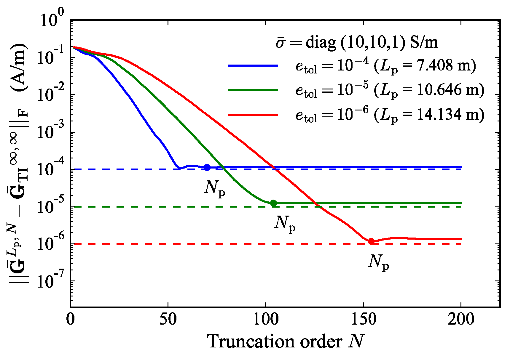
2.2.4. Tensor Green’s Function and the Choice of Region’s Size and Truncation Order

In the previous subsections, we derived the spatial-domain EM fields E ( r ) , H ( r ) produced by a single magnetic dipole source M δ ( r r ) . Allowing M = x ^ ,   y ^ ,   z ^ successively, we can compute the corresponding magnetic fields H x ,   H y ,   H z due to the three mutually orthogonal unit sources. Their combination produces the spatial-domain magnetic Green’s function, i.e.,
G ¯ ( r , r ) = [ H x , H y , H z ] = [ H x x H x y H x z H y x H y y H y z H z x H z y H z z ]
where H p q denotes the p-component of the magnetic field due to the unit source in the q-axis direction. Using (28), we can also write the Green’s function as a Fourier series,
G ¯ ( r , r ) = n = m = F ¯ n m H L ¯ n m W ¯ n m e i ( k n x + k m y )
where the 4 × 3 matrix W ¯ n m = [ w n m , x , w n m , y , w n m , z ] represents the combination of the mode-waves corresponding to the three sources.
In practice, we can calculate the finite series in (31) by taking its partial sum, i.e.,
G ¯ ( r , r ) G ¯ L , N ( r , r ) = n = N N m = N N F ¯ n m H L ¯ n m W ¯ n m e i ( k n x + k m y )
where the superscripts L and N are used to signify the region’s size and the truncation order, respectively. Using the notation of partial sum, the FRA solution in (31) can be expressed as a limit when N , i.e.,
G ¯ ( r , r ) = lim N G ¯ L , N ( r , r ) = G ¯ L , ( r , r )
When L , the FRA solution further becomes the exact solution of the original problem in the entire space,
G ¯ exact ( r , r ) = lim L G ¯ L , ( r , r ) = G ¯ , ( r , r )
Therefore, we will use the unified notation with double superscripts to express the three solutions: the FRA solution G ¯ L , , the approximate solution G ¯ L , N , and the exact solution G ¯ , . The total error of the approximate solution G ¯ L , N can then be divided into two parts,
Δ ¯ total L , N = G ¯ L , N G ¯ , = [ G ¯ L , N G ¯ L , ] + [ G ¯ L , G ¯ , ] = Δ ¯ spectral + Δ ¯ spatial .
Here, Δ ¯ spatial = G ¯ L , G ¯ , represents the reflections from the four truncation planes, which is caused by the finite L , which we call the spatial truncation error, whereas Δ ¯ spectral = G ¯ L , N G ¯ L , is the spectral truncation error caused by the finite N . We first study the spatial truncation error.
For simplicity, we assume that the source is located at r 0 = ( 0 , 0 , 0 ) in an unbounded medium. As shown in Figure 2a,b, G ¯ , is the solution to a free-space problem, whereas G ¯ L , can be regarded as the solution to a boundary-value problem in Ω subject to the boundary conditions (29). Using the method of images, we can construct an equivalent free-space problem to the problem in Figure 2b by introducing an infinite number of image sources with the same magnitude and direction as the original source. As shown in Figure 2c, these sources are located at
r p q = r 0 + ( 2 p L , 2 q L , 0 ) ,   p ,   q
The one located at r 0 , 0 = r 0 Ω represents the original source (shown in red dot) and the rest located at r p q Ω represent the image sources (shown in green dots). It is easy to verify that the sum of the contributions due to the original source and its image sources satisfies the conditions in (29). By the uniqueness theorem, we conclude that the problem in Figure 2c is equivalent to the problem in Figure 2b. Thus, the FRA solution G ¯ L , can be expressed as
G ¯ L , ( r , r 0 ) = q = + p = + G ¯ , ( r , r p q ) = G ¯ , ( r , r 0 ) + r p q Ω G ¯ , ( r , r p q ) ,   r Ω
From (37), we obtain the following expression for the spatial truncation error:
Δ ¯ spatial = G ¯ L , ( r , r 0 ) G ¯ , ( r , r 0 ) = r p q Ω G ¯ , ( r , r p q ) ,   r Ω .
To measure the magnitude of a tensor, we introduce the following Frobenius norm for an arbitrary 3 × 3 tensor A ¯ with entries a i j ,   i ,   j = 1 ,   2 ,   3 :
A ¯ F = j = 1 3 i = 1 3 | a i j | 2
Taking the norm of (38) and using the triangle inequality, we have
Δ ¯ spatial F r p q Ω G ¯ , ( r , r p q ) F ,   r Ω
The right-hand side of (40) gives an upper bound for the spatial truncation error. When the medium is isotropic, each term of can be calculated by using the exact formula of the magnetic Green’s function in the free space [31]:
G ¯ iso , ( r , r ) = k 2 e i k R 4 π R [ 1 + i k R 1 k 2 R 2 ] I ¯ k 2 e i k R 4 π R [ 1 + 3 i k R 3 k 2 R 2 ] ( r r R ) ( r r R )
where k = i ω μ ( σ i ω ε ) , R = | r r | , I ¯ = x ^ x ^ + y ^ y ^ + z ^ z ^ is the identity dyad. We use (41) to estimate the influence the computational region’s size L on the EM fields and further develop a principle to choose the proper L even for the anisotropic media.
Consider a specific case as an example: the observer is located at r = 1.016 × ( 1 / 2 , 0 , 3 / 2 )   m , and the frequency of the source is 20   kHz . The right-side of (40) only depends on the variables σ and L ; thus, we can define it as the following function:
f ( σ , L ) = r p q Ω G ¯ iso , ( r , r p q ) F
Its P-th ( P = 1 ,   2 ,   ,   ) order approximation can be defined as
f P ( σ , L ) = r p q Ω , max { | p | , | q | } P G ¯ iso , ( r , r p q ) F
which represents the contributions of the ( 2 P + 1 ) 2 1 image sources nearest to the original source. Figure 3 shows the graph of f P ( σ , L ) when P is equal to four different values 1, 2, 3 and 1000 in the case of σ = 1   S / m . From the results, we can observe that f P ( σ , L ) converges quickly with the increase in P and the values of f 3 ( σ , L ) becoming almost consistent with that of f 1000 ( σ , L ) . Thus, we choose f 3 ( σ , L ) to approximate f ( σ , L ) to investigate the influence of region size L . The whole graph of f 3 ( σ , L ) in Figure 4 demonstrates that f 3 ( σ , L ) decreases monotonically with the decrease in σ and L . If the conductivity σ is known and some error tolerance denoted by e tol is given, we can find a unique proper value of L , denoted by L p , such that
f 3 ( σ , L p ) = e tol
Theoretically, the above principle of choosing L p can ensure that the spatial truncation error does not exceed e tol . Considering a medium of σ = 1   S / m , Figure 4 illustrates the corresponding choices Lp = 7.408, 10.646, 14.134 m for meeting the three different error tolerances e tol = 10 4 ,   10 5 ,   10 6 . Figure 5 further shows the changes in the total error of the approximate solution G ¯ L p , N with the truncation order N ranging from 1 to 200 for the three different values of L p . The error is defined by
Δ ¯ total L p , N F = G ¯ L p , N ( r , r 0 ) G ¯ iso , ( r , r 0 ) F
We can observe that there exists a proper truncation order N p for each case of L p , and the total error of G ¯ L p , N no longer decreases after N is up to N p . This observation indicates the following results:
G ¯ L p , N p = G ¯ L p , N = G ¯ L p , ,   N N p
That is, G ¯ L p , N p has arrived at the value of G ¯ L p , , and the spectral truncation error Δ ¯ spectral = G ¯ L p , N p G ¯ L p , can be ignored. Consequently, the total error of G ¯ L p , N p is equal to the spatial truncation error, which will not exceed the present error tolerance e tol , i.e.,
Δ ¯ total L p , N p F = Δ ¯ spatial F f 3 ( σ , L p ) = e tol
The numerical results in Figure 5 confirm this conjecture. In a practical calculation, we can determine N p as the smallest N that meets the following stopping criterion:
G ¯ L p , N G ¯ L p , N 2 F G ¯ L p , N F < 0.01 × e tol
and take G ¯ L p , N p as the final result.
For the case of the anisotropic medium (including TI and BA cases) with tensor conductivity σ ¯ , we can take σ ˜ = min { σ x p , σ y p , σ z p } as the approximate isotropic conductivity, where σ x p ,   σ y p ,   σ z p are the three principal components of tensor σ ¯ . The previous principles for determining L p and N p , which is based on the isotropic model, can then be generalized to the anisotropic case as well. Considering a TI medium of σ ¯ = diag ( 10 , 10 , 1 )   S / m , Figure 6 presents the total error of G ¯ L p , N as the truncation order N increases for the three L p determined by e tol = 10 4 , 10 5 ,   10 6 . The total error is calculated by
Δ ¯ total L p , N F = G ¯ L p , N ( r , r 0 ) G ¯ TI , ( r , r 0 ) F
where G ¯ TI , is the exact solution of the magnetic Green’s function in an unbounded TI medium, and its formula can be found in [32]. For this medium, although we cannot guarantee that the error of approximate solution G ¯ L p , N p is less than the present e tol , the results in Figure 6 demonstrate that the error is close to the present e tol . Thus, we still apply previous principles to determine L p and N p for the anisotropic media. For a J-layer anisotropic medium, we may take min { σ ˜ 1 ,   ,   σ ˜ j ,   ,   σ ˜ J } as the approximate isotropic conductivity, where σ ˜ j is the minimum of the three principal components of the conductivity in layer j . In the following section, the error tolerance will be fixed at e tol = 10 5 .

3. Results

In this section, we apply the proposed FRA to simulate the responses of the triaxial logging tool in the layered TI and BA formations. As shown in Figure 7a, the tool is equipped with three mutually orthogonal transmitters T x ,   T y ,   T z and three mutually orthogonal receivers R x ,   R y ,   R z . Figure 7b illustrates the orientation of the tool coordinates x t y t z t with respect to the formation coordinates x y z : the y t -axis is assumed to be parallel to the x y -plane and the z t -axis points to the direction from the transmitters to receivers. The rotation matrix from x y z to x t y t z t can be expressed as
R ¯ = [ cos α sin α 0 sin α cos α 0 0 0 1 ] × [ cos θ 0 sin θ 0 1 0 sin θ 0 cos θ ]
where α and θ represent the azimuthal and dip angles of the tool. To simulate the responses of the triaxial logging tool, the magnetic Green’s function in (30) should be converted into the tool coordinates by
G ¯ t = [ H x x t H x y t H x z t H y x t H y y t H y z t H z x t H z y t H z z t ] = R ¯ T G ¯ R ¯
where H p q t ( p , q = x , y , z ) denotes the response of the receiver R p due to the transmitter T q . In the following results, the offset-spacing, the operating frequency and the azimuthal angle of the triaxial logging tool will be fixed at 1.016 m, 20 kHz and 0°, respectively. The superscript “t” of response H p q t will be omitted for brevity.
As shown in Figure 8, a five-layer anisotropic model is assumed, where the thicknesses of the three middle layers are 2, 2 and 4 m, respectively. The layers 1, 3 and 5 are assumed to be isotropic, and the conductivities are 0.1, 0.1 and 0.05 S/m, respectively. The conductivities in layers 2 and 4 share the identical tensor conductivity σ ¯ , which is assumed to be TI or BA.

3.1. Triaxial Logging Responses in Layered TI Media

To validate this new algorithm, we compare the results by the present FRA with those of the TLM [30] in a TI formation. The five-layer model in Figure 8 is considered, where the conductivity σ ¯ of layers 2 and 4 is assumed to be TI and is equal to diag ( 1 , 1 , 0.1 )   S / m . Two different tool dip angles θ = 60° and θ = 89° are considered. We will only provide the results of the components Im H x x ,   Im H y y ,   Im H z z ,   Im H x z ,   Im H z x because the remaining Im H x y ,   Im H y x ,   Im H y z ,   Im H z y are all zeros. Figure 9 and Figure 10 show the comparison with the TLM for the cases of θ = 60° and θ = 89°, respectively. The corresponding relative errors are displayed in Figure 9f and Figure 10f. The relative error of each component is less than 2% except for a few sampling points (where the absolute value of response is close to zero). The excellent agreements validate our algorithm. The direct summation of the Fourier series for the case of θ = 89° exhibits a weakly convergent behavior, and the required summation order will be extremely large. This difficulty is solved by using the singularity subtraction [13,21]. Furthermore, from Figure 9 and Figure 10, we can find that the local extremums of the cross components Im H x z and Im H z x can clearly indicate the location of the interfaces for both cases.
To further validate the present algorithm in formation with a high conductivity, we assume the conductivity of layers 2 and 4 to be σ ¯ = diag ( 20 , 20 , 2 )   S / m and the tool dip angle to be θ = 60 ° . Figure 11 shows the comparison with the TLM. The agreement validates our algorithm again.

3.2. Triaxial Logging Responses in Layered BA Media

Here, we further investigate the response of the triaxial logging tool in the BA formations. The five-layer model in Figure 8 is still considered, where the conductivity σ ¯ of layers 2 and 4 is assumed to be BA. The three specific BA conductivities shown in Figure 11 are considered. All of them share the same principal conductivity diag ( 4 ,   1 ,   0.5 )   S / m . The orientations of their principal coordinates x p y p z p with respect to the formation coordinates x y z are also illustrated in Figure 12: the principal coordinates x p y p z p of the simple BA case are consistent with x y z ; those of the dipping BA case have an anisotropic dip angle γ = 15 ° ; those of the Full-tensor BA case have an anisotropic azimuthal angle β = 15 ° and an anisotropic dip angle γ = 15 ° . The tool dip angle is fixed at θ = 60 ° . For the simple BA and dipping BA cases, Figure 13 only displays the results of components Im H x x ,   Im H y y ,   Im H z z ,   Im H x z , Im H z x , because the rest are all zeros. Note that in these two cases, the tool dip angle and the anisotropic dip angle are in the same x z -plane. However, in the cases of full-tensor BA conductivity, this condition no longer holds because of the anisotropic azimuthal angle. The results in Figure 14 show that none of the nine responses are zero. Furthermore, comparing the results of the dipping BA ( γ = 15 ° ) case with those of the simple BA ( γ = 0 ° ) case, we can observe that the three main components Im H x x ,   Im H y y , and Im H z z are sensitive to the change in the anisotropic dip angle γ . These differences among the results of the three cases indicate that the orientation of BA conductivity has a significant influence on the responses of the triaxial logging tool. To obtain a more reliable interpretation of logging data, this effect should be considered.

4. Conclusions

This paper presents a new algorithm of the EM fields in the layered BA media. We solved Maxwell’s equations in a rectangular region with a finite cross-section. Since the solution was expressed as a 2-D Fourier series, its evaluation can be implemented by a simple summation without resorting to the additional numerical quadrature algorithms. Using the method of images, we also developed a quantitative principle to choose the proper size of the region according to the desired error tolerance. Our algorithm was applied to simulate responses of the triaxial well logging tool in layered TI and BA formations, and the numerical results are compared with those by the other method. The excellent agreements demonstrate that this algorithm can effectively and accurately simulate the responses of the triaxial logging tool in normally or highly deviated wells.

Author Contributions

Conceptualization, Z.K. and H.W.; methodology, Z.K. and H.W.; formal analysis, Z.K., H.W. and C.Y.; writing—original draft preparation, Z.K.; writing—review and editing, H.W. and C.Y. All authors have read and agreed to the published version of the manuscript.

Funding

This research was funded by the Strategic Priority Research Program of the Chinese Academy of Sciences under grant XDA14020102, the National Natural Science Foundation of China under grant 42174150, the Jilin Province Science and Technology Development Program under grant YDZJ202102CXJD016.

Institutional Review Board Statement

Not applicable.

Informed Consent Statement

Not applicable.

Data Availability Statement

The data included in this study are available from the corresponding author upon reasonable request.

Conflicts of Interest

The authors declare no conflict of interest.

Appendix A

By the proper normalization, the eigenvector matrix for layer j and its inverse matrix can be expressed in terms of the four 2 × 2 matrices L ¯ j , I ,   L ¯ j , II ,   L ¯ j , III ,   L ¯ j , VI (the detailed expressions can be found in [15]) and they transpose the matrices as follows:
L ¯ j = 1 2 [ L ¯ j , I L ¯ j , II L ¯ j , III L ¯ j , VI ] ,   L ¯ j 1 = 1 2 [ L ¯ j , III T L ¯ j , I T L ¯ j , VI T L ¯ j , II T ]
Consider a two-layer model and assume an incident downward wave with amplitude A + hitting the interface z 2 from upper layer 1 into lower layer 2. The mode-waves in these two layers are
w 1 = [ e i ω Λ ¯ 1 u ( z z 2 ) R ¯ 1 , 2 e i ω Λ ¯ 1 d ( z z 2 ) ] A +
w 2 = [ 0 e i ω Λ ¯ 2 d ( z z 2 ) T ¯ 1 , 2 ] A +
where R ¯ 1 , 2 and T ¯ 1 , 2 are the unknown local reflection and transmission coefficients, respectively. To determine these coefficients, we apply continuity conditions across the interface z 2 , i.e.,
b ( z 2 ) = b ( z 2 + )
where z 2 ( z 2 + ) represent the left (right) limit of z 2 . Using the relation b = L ¯ w and expressions in (A2) and (A3), the condition can be written as
L ¯ 1 [ R ¯ 1 , 2 I ¯ ] = L ¯ 2 [ 0 T ¯ 1 , 2 ]
Substituting (A1) into (A5) and solving this equation for R ¯ 1 , 2 and T ¯ 1 , 2 , we have
T ¯ 1 , 2 = 2 [ L ¯ VI , 1 T L ¯ II , 2 + L ¯ II , 1 T L ¯ VI , 2 ] 1 R ¯ 1 , 2 = [ L ¯ III , 1 T L ¯ II , 2 L ¯ I , 1 T L ¯ VI , 2 ] × [ L ¯ VI , 1 T L ¯ II , 2 + L ¯ II , 1 T L ¯ VI , 2 ] 1
Similarly, assuming that an incident upward wave hits interface z 2 from the lower layer 2, and after a similar derivation, we obtain
T ¯ 2 , 1 = 2 [ L ¯ III , 2 T L ¯ I , 1 + L ¯ I , 2 T L ¯ III , 1 ] 1 R ¯ 2 , 1 = [ L ¯ VI , 2 T L ¯ I , 1 L ¯ II , 2 T L ¯ III , 1 ] × [ L ¯ III , 2 T L ¯ I , 1 + L ¯ I , 2 T L ¯ III , 1 ] 1

References

  1. Ursin, B. Review of elastic and electromagnetic wave propagation in horizontally layered media. Geophysics 1983, 48, 1063–1081. [Google Scholar] [CrossRef]
  2. Zhong, Y.; Lambert, M.; Lesselier, D.; Chen, X. Electromagnetic response of anisotropic laminates to distributed sources. IEEE Trans. Antennas Propag. 2014, 62, 247–256. [Google Scholar] [CrossRef]
  3. Yin, C. MMT forward modeling for a layered earth with arbitrary anisotropy. Geophysics 2006, 71, G115–G128. [Google Scholar] [CrossRef]
  4. Howard, A.Q. Petrophysics of magnetic dipole fields in an anisotropic earth. IEEE Trans. Antennas Propag. 2000, 48, 1376–1383. [Google Scholar] [CrossRef]
  5. Yu, L.; Wang, H.; Wang, H.; Yang, S.; Yin, C. 3-D finite volume modeling for LWD azimuthal propagation resistivity tool with multiple annular antenna recesses using coupled potentials on cylindrical grids. IEEE Trans. Antennas Propag. 2022, 70, 514–525. [Google Scholar] [CrossRef]
  6. Li, D.; Wilton, D.R.; Jackson, D.R.; Wang, H.; Chen, J. Accelerated computation of triaxial induction tool response for arbitrarily deviated wells in planar-stratified transversely isotropic formations. IEEE Geosci. Remote Sens. Lett. 2018, 15, 902–906. [Google Scholar] [CrossRef]
  7. Xing, G.; Zhang, X.; Teixeira, F.L. Computation of tensor Green’s functions in uniaxial planar-stratified media with a rescaled equivalent boundary approach. IEEE Trans. Antennas Propag. 2018, 66, 1863–1873. [Google Scholar] [CrossRef]
  8. Wang, H.N.; Yu, L.; Wang, H.S.; Yang, S.W.; Yin, C.C. A hybrid algorithm for LWD azimuthal electromagnetic responses with annular grooved drill collar. Chin. J. Geophys. 2021, 64, 1811–1829. [Google Scholar] [CrossRef]
  9. Lee, H.O.; Teixeira, F.L. Cylindrical FDTD analysis of LWD tools through anisotropic dipping-layered earth media. IEEE Trans. Geosci. Remote Sens. 2007, 45, 383–388. [Google Scholar] [CrossRef]
  10. Chew, W.C.; Chen, S.-Y. Response of a point source embedded in a layered medium. IEEE Antennas Wirel. Propag. Lett. 2003, 2, 254–258. [Google Scholar] [CrossRef] [Green Version]
  11. Hong, D.; Xiao, J.; Zhang, G.; Yang, S. Characteristics of the sum of cross-components of triaxial induction logging tool in layered anisotropic formation. IEEE Trans. Geosci. Remote Sens. 2014, 52, 3107–3115. [Google Scholar] [CrossRef]
  12. Michalski, K.A.; Mosig, J.R. Multilayered media Green’s functions in integral equation formulations. IEEE Trans. Antennas Propagat. 1997, 45, 508–519. [Google Scholar] [CrossRef]
  13. Simsek, E.; Liu, Q.H.; Wei, B. Singularity subtraction for evaluation of Green’s functions for multilayer media. IEEE Trans. Microw. Theory Tech. 2006, 54, 216–225. [Google Scholar] [CrossRef]
  14. Chew, W.C. Waves and Fields in Inhomogenous Media; Wiley-IEEE Press: New York, NY, USA, 1995. [Google Scholar]
  15. Løseth, L.O.; Ursin, B. Electromagnetic fields in planarly layered anisotropic media. Geophys. J. Int. 2007, 170, 44–80. [Google Scholar] [CrossRef] [Green Version]
  16. Morgan, M.; Fisher, D.; Milne, E. Electromagnetic scattering by stratified inhomogeneous anisotropic media. IEEE Trans. Antennas Propag. 1987, 35, 191–197. [Google Scholar] [CrossRef]
  17. Yang, H.D. A spectral recursive transformation method for electromagnetic waves in generalized anisotropic layered media. IEEE Trans. Antennas Propag. 1997, 45, 520–526. [Google Scholar] [CrossRef]
  18. Hong, D.; Li, N.; Han, W.; Zhan, Q.; Zeyde, K.; Liu, Q.H. An analytic algorithm for dipole electromagnetic field in fully anisotropic planar-stratified media. IEEE Trans. Geosci. Remote Sens. 2021, 59, 9120–9131. [Google Scholar] [CrossRef]
  19. Hu, X.; Fan, Y.; Deng, S.; Yuan, X.; Li, H. Electromagnetic logging response in multilayered formation with arbitrary uniaxially electrical anisotropy. IEEE Trans. Geosci. Remote Sens. 2020, 58, 2071–2083. [Google Scholar] [CrossRef]
  20. Sainath, K.; Teixeira, F.L. Tensor Green’s function evaluation in arbitrarily anisotropic layered media using complex-plane Gauss-Laguerre quadrature. Phys. Rev. E 2014, 89, 053303. [Google Scholar] [CrossRef] [Green Version]
  21. Hu, Y.; Fang, Y.; Wang, D.; Zhong, Y.; Liu, Q.H. Electromagnetic waves in multilayered generalized anisotropic media. IEEE Trans. Geosci. Remote Sens. 2018, 56, 5758–5766. [Google Scholar] [CrossRef]
  22. Li, N.; Hong, D.; Han, W.; Liu, Q.H. An analytic algorithm for electromagnetic field in planar-stratified biaxial anisotropic formation. IEEE Trans. Geosci. Remote Sens. 2020, 58, 1644–1653. [Google Scholar] [CrossRef]
  23. He, Z.; Huang, K.; Liu, R.C.; Guo, C.; Jin, Z.; Zhang, L. A semianalytic solution to the response of a triaxial induction logging tool in a layered biaxial anisotropic formation. Geophysics 2016, 81, D71–D82. [Google Scholar] [CrossRef]
  24. Kang, Z.Z.; Wang, H.N.; Wang, H.-S.; Yang, S.-W.; Yin, C.C. Study of multi-component induction logging in layered crossbedding formations by using propagation matrix method. Chin. J. Geophys. 2020, 63, 4277–4289. [Google Scholar] [CrossRef]
  25. Yao, D.H.; Wang, H.N.; Yang, S.W.; Yang, H.L. Study on the responses of multi-component induction logging tool in layered orthorhombic anisotropy formations by using propagator matrix method. Chin. J. Geophys. 2010, 53, 3026–3037. [Google Scholar]
  26. Wang, H.; Tao, H.; Yao, J.; Zhang, Y. Efficient and reliable simulation of multicomponent induction logging response in horizontally stratified inhomogeneous TI formations by numerical mode matching method. IEEE Trans. Geosci. Remote Sens. 2012, 50, 3383–3395. [Google Scholar] [CrossRef]
  27. Wang, G.L.; Barber, T.; Wu, P.; Allen, D.; Abubakar, A. Fast inversion of triaxial induction data in dipping crossbedded formations. Geophysics 2017, 82, D31–D45. [Google Scholar] [CrossRef]
  28. Wang, H. Adaptive regularization iterative inversion of array multicomponent induction well logging datum in a horizontally stratified inhomogeneous TI formation. IEEE Trans. Geosci. Remote Sens. 2011, 49, 4483–4492. [Google Scholar] [CrossRef]
  29. Kang, Z.; Wang, H.; Wang, Y.; Yin, C. Fourier series approximation of tensor Green’s function in biaxial anisotropic media. IEEE Geosci. Remote Sens. Lett. 2022, 19, 1–5. [Google Scholar] [CrossRef]
  30. Yang, S.; Wang, J.; Zhou, J.; Zhu, T.; Wang, H. An efficient algorithm of both Fréchet derivative and inversion of MCIL data in a deviated well in a horizontally layered TI formation based on TLM modeling. IEEE Trans. Geosci. Remote Sens. 2014, 52, 6911–6923. [Google Scholar] [CrossRef]
  31. Kong, J.A. Electromagnetic Waves Theory; EMW Publishing: Cambridge, UK, 2000. [Google Scholar]
  32. Zhdanov, M.S.; Kennedy, W.D.; Peksen, E. Foundation of the tensor induction well logging. Petrophysics 2001, 42, 588–610. [Google Scholar]
Figure 1. The infinitely long rectangular region with a square cross-section and a layered anisotropic medium.
Remotesensing 14 03836 g001
Figure 2. Schematic of the three related problems, where the red dot and the green dots represent the original source and the image sources, respectively. (a) Original free-space problem. (b) Boundary-value problem of the proposed FRA. (c) Equivalent free-space problem to the problem in (b).
Remotesensing 14 03836 g002
Figure 3. P-th order approximation f P ( σ , L ) of the infinite series f ( σ , L ) for the four different P = 1 ,   2 ,   3 and 1000.
Remotesensing 14 03836 g003
Figure 4. The graph of the function f 3 ( σ , L ) and the illustration of the process for choosing proper region size.
Remotesensing 14 03836 g004
Figure 5. Error of G ¯ L p , N with increasing truncation order N for three cases of L p when the medium is isotropic.
Remotesensing 14 03836 g005
Figure 6. Error of G ¯ L p , N with increasing truncation order N for three cases of L p when the medium is anisotropic.
Remotesensing 14 03836 g006
Figure 7. Triaxial logging tool and its orientation. (a) Structure of the tool in the tool coordinates x t y t z t . (b) Orientation of the tool coordinates x t y t z t with respect to the formation coordinates x y z , where α and θ are the tool azimuthal and dip angles, respectively.
Remotesensing 14 03836 g007
Figure 8. Five-layer anisotropic model and two deviated well logging trajectories in the formation coordinates x y z . Layers 2 and 4 share the same tensor conductivity σ ¯ .
Remotesensing 14 03836 g008
Figure 9. Responses of the tool with dip angle θ = 60 ° simulated by TLM and the present method. (a) Im ( H x x ) . (b) Im ( H y y ) . (c) Im ( H z z ) . (d) Im ( H x z ) . (e) Im ( H z x ) . (f). Relative error.
Remotesensing 14 03836 g009
Figure 10. Responses of the tool with dip angle θ = 89 ° simulated by the TLM and present method. (a) Im ( H x x ) . (b) Im ( H y y ) . (c) Im ( H z z ) . (d) Im ( H x z ) . (e) Im ( H z x ) . (f). Relative error.
Remotesensing 14 03836 g010
Figure 11. Responses of the tool in the layered model with σ ¯ = diag ( 20 , 20 , 2 )   S / m simulated by the TLM and present method. (a) Im ( H x x ) . (b) Im ( H y y ) . (c) Im ( H z z ) . (d) Im ( H x z ) . (e) Im ( H z x ) . (f). Relative error.
Remotesensing 14 03836 g011
Figure 12. Three specific BA conductivities and the orientations of the principal coordinates x p y p z p with respect to the formation coordinates x y z , where β and γ are the anisotropic azimuthal and dip angles (similar to the definition of α and θ in Figure 7b), respectively. (a) Simple BA. (b) Dipping BA. (c) Full-tensor BA.
Remotesensing 14 03836 g012
Figure 13. Responses of the tool in the layered simple BA and dipping BA formations. (a) Im ( H x x ) . (b) Im ( H y y ) . (c) Im ( H z z ) . (d) Im ( H x z ) . (e) Im ( H z x ) .
Remotesensing 14 03836 g013
Figure 14. Responses of the tool in the layered full-tensor BA formation. (a) Im ( H x x ) . (b) Im ( H x y ) . (c) Im ( H x z ) . (d) Im ( H y x ) . (e) Im ( H y y ) . (f) Im ( H y z ) . (g) Im ( H z x ) . (h) Im ( H z y ) . (i) Im ( H z z ) .
Remotesensing 14 03836 g014
Publisher’s Note: MDPI stays neutral with regard to jurisdictional claims in published maps and institutional affiliations.

