1. Introduction
For Network Real Time Kinematic (NRTK), ambiguity resolution at Continuously Operating Reference Station (CORS) network sites is the key step in the whole processing chain, which culminates in generating ionospheric corrections at the user site; therefore, the speed of successful ambiguity resolution is important for NRTK, and single-epoch ambiguity resolution is the ultimate goal. With single-epoch ambiguity resolution, NRTK can recover instantaneously after maintenance or breakdown, and cycle slip will no longer be a problem, which may be important in low- or high-latitude areas in the case of ionospheric scintillations.
Unfortunately, single-epoch ambiguity resolution has not been realized till now especially for large-scale CORS networks. The most important reason is that, traditionally, ambiguity will be estimated together with tropospheric delay and these two kinds of parameters are highly correlated, which affects single-epoch ambiguity resolution performance severely [
1,
2]. So, with multiple-frequency observations available, the tropospheric delay becomes the dominant error source affecting single-epoch ambiguity resolution performance, especially for large-scale NRTK [
3]. And the best, and possibly the only, feasible way of dealing with tropospheric delay is to find a method to neglect the tropospheric delay as much as possible.
In our previous research [
4], a method of neglecting tropospheric delay by forming difference between satellites with close mapping functions was proposed. The effect of the method depends on the density of mapping functions. In our previous research, the difference is formed between satellites within the same GNSS and the density of mapping functions is not enough to neglect zenith tropospheric delay as big as several centimeters, so it is only applicable to small-scale CORS networks.
In recent years, with the launch of Galileo [
5] and BeiDou [
6,
7], and with the modernization of GPS and GLONASS [
8,
9,
10,
11], multi-frequency signals have become available for every GNSS. Most importantly, the civil signals on L1/1575.42 and L5/1176.45 are all available on GPS, Galileo and BeiDou [
12]. It provides an opportunity to form difference between satellites of different GNSSs. It means that the mapping functions will become much denser, and the ability to neglect zenith tropospheric delay will certainly be improved. So, single-epoch ambiguity resolution for large-scale CORS networks may be feasible in the future.
Thus, in this research, a new method is developed to explore the full potential of multi-frequency and multi-constellation GNSSs, especially for the L1 and L5 shared carrier phase types of GPS, Galileo and BeiDou. The core part of the method is forming difference between satellites with close mapping functions whether they belong to same or different GNSSs. The biggest obstacle to overcome is to get the single-epoch ambiguity solution for wide-lane combinations of L1 and L5 when the difference is formed between satellites of different GNSSs. The proposed method includes five steps: extra wide-lane ambiguity resolution, wide-lane ambiguity resolution, inter-GNSS wide-lane ambiguity resolution, subset narrow-lane ambiguity resolution and full narrow-lane ambiguity resolution. Numerical test results are given with the description of every ambiguity-resolution step.
3. Proposed CORS Ambiguity-Resolution Method
In this section, the proposed CORS ambiguity-resolution method is introduced. It is a cascading ambiguity-resolution scheme and five steps are involved. Example numerical results will be given together with a detailed description of each step based on the observations from two IGS stations, BRUX (4.4°E, 50.8°N) and REDU (5.1°E, 50.0°N), separated by a baseline distance of approximately 104 km. The two receivers are both SEPT POLARX5TR, the observation date was 9 May 2020 and the sample interval is 30 s. During pre-processing, the Hopefield troposphere model is applied.
- (1)
Extra-wide-lane ambiguity resolution
The ambiguity-resolution method of extra-wide lanes is based on the MW combination [
13,
14], which is traditionally used:
where
;
;
and
are frequencies;
and
are wavelengths;
and
are corresponding phase observations;
and
are corresponding code observations; and
is the estimated integer extra-wide-lane ambiguity.
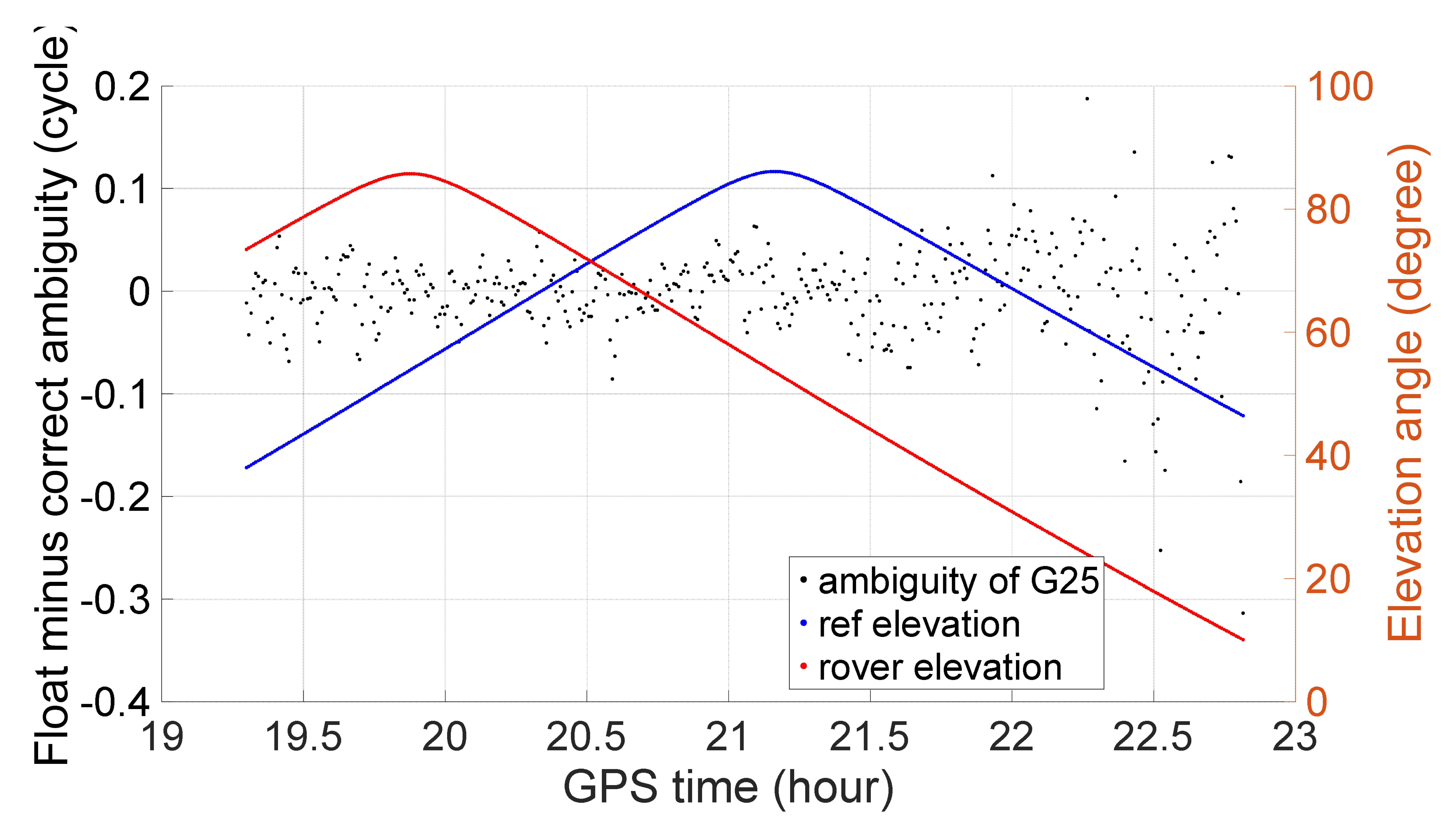
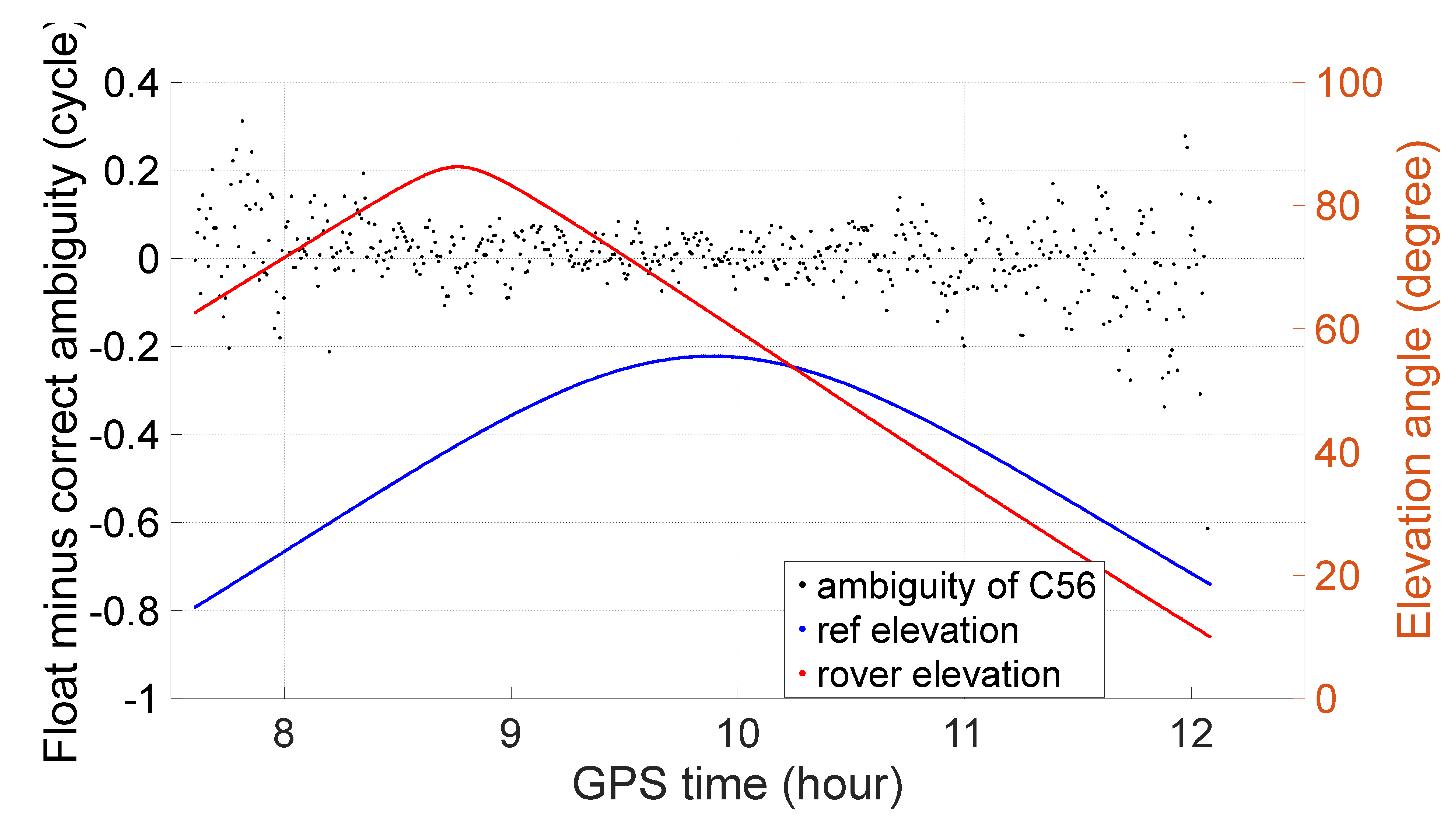
Taking extra-wide lanes G25, C56 and E56 as examples,
Figure 1,
Figure 2 and
Figure 3 show the float ambiguity minus the correct ambiguity and the corresponding elevation angles of the reference and rover satellites. The values are all below a quarter cycle except when the elevation angle is below or approximately 15°. Most of them can be fixed correctly with a threshold of 0.25 cycles, and there will be no misfixed case.
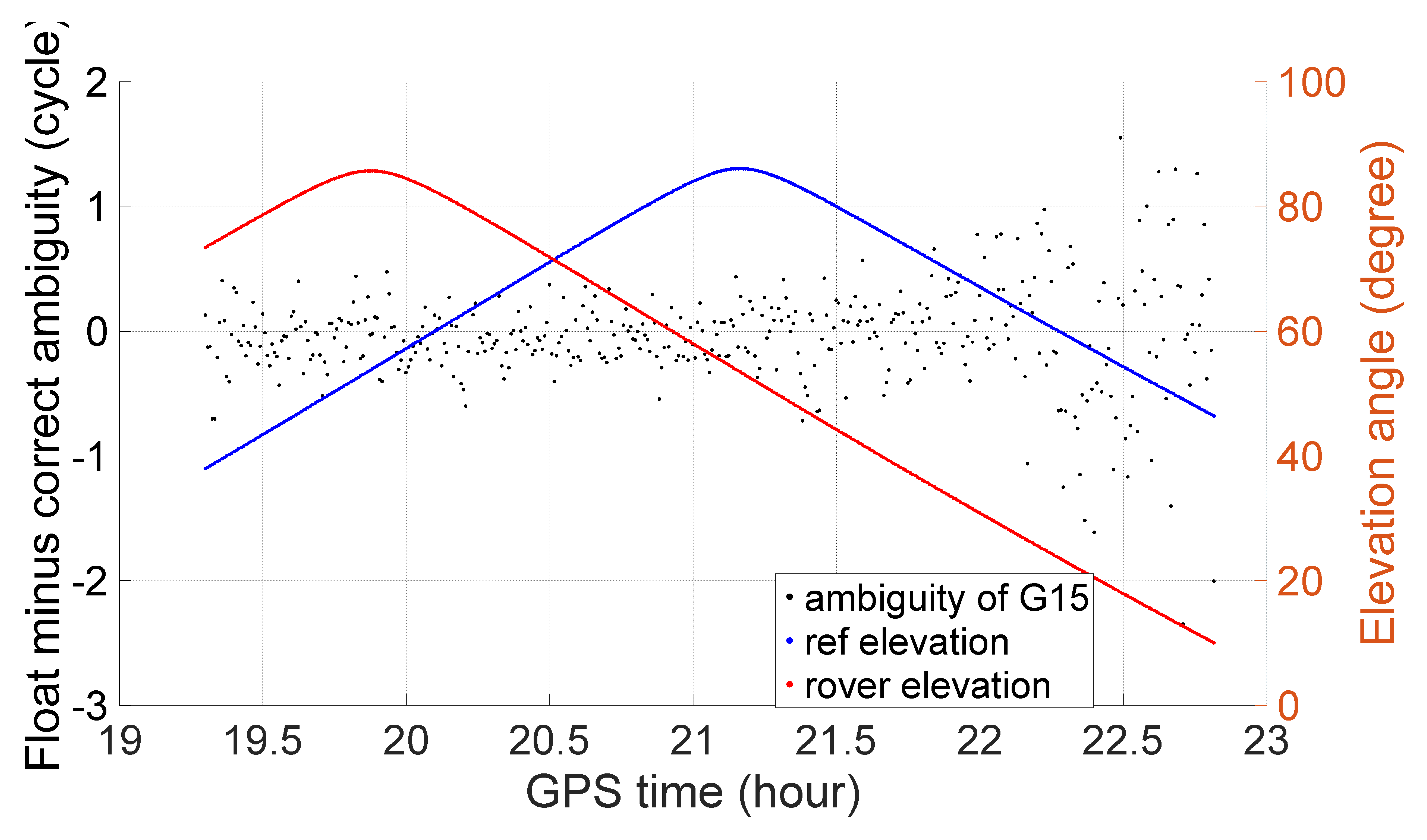
For comparison, three wide lanes, G15, C15 and E15, are also taken as examples, and their float ambiguity minus the correct ambiguity is shown in
Figure 4,
Figure 5 and
Figure 6. Compared to those of the extra-wide lane, their values are much larger and scattered. When fixing them with a threshold of 0.25 cycles, many cases cannot be fixed and there are also many cases that are misfixed.
Table 5,
Table 6 and
Table 7 show the statistics of the wide-lane ambiguity-resolution performance of GPS, BeiDou and Galileo with a threshold of 0.25 cycles. With an extra-wide lane, more than 97 percent can be fixed successfully; some can be 100% fixed and there is no misfixation. However, with a wide lane only approximately 50% can be fixed. All of them have misfixed cases and some can reach more than 10%. Therefore, we can conclude that with an extra-wide lane, single-epoch ambiguity resolution based on WM combinations is feasible and reliable, while with a wide lane it is not feasible.
- (2)
Wide-lane ambiguity resolution
To realize single-epoch wide-lane ambiguity resolution, the following mathematical model is proposed:
where
,
and
are carrier phase observations of frequency bands
,
and the extra-wide lane;
is ionospheric delay;
,
&
are corresponding coefficients;
and
are the ambiguity of frequency bands
&
;
&
are corresponding wavelengths;
is the fixed extra-wide-lane ambiguity resolution; and
is the wavelength. Note that
.
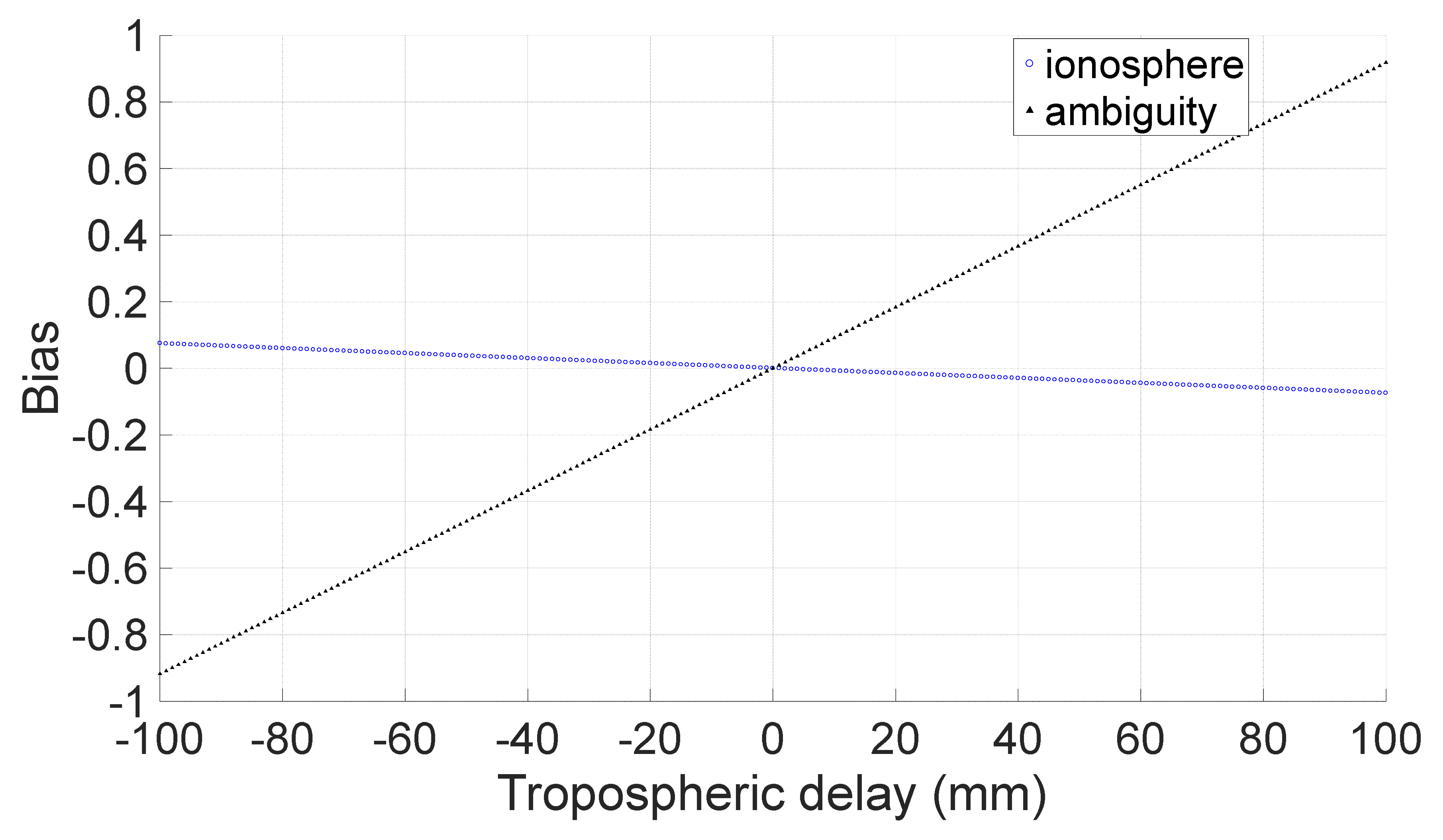
Note that in the above equations tropospheric delay is ignored, and its effect on ambiguity resolution is investigated by simulation. Taking GPS as an example, the above mathematical model will become
where
is the ignored tropospheric delay; the weight matrix is formed according to the carrier phase and code noise (3 mm and 0.3 m, respectively). By assigning different values to
from −0.5 m to 0.5 m and resolving the above equation with the least-squares adjustment, the resulting bias of the estimated narrow-lane ambiguity resolution, wide-lane ambiguity resolution (unit: cycle) and ionospheric delay (unit: m) due to ignored tropospheric delay was determined, as shown in
Figure 7.
From
Figure 7 we can see that the effect of the ignored tropospheric delay on the estimation of wide-lane ambiguity is very small at only approximately 0.1 cycles, even with ignored tropospheric delays as large as 0.5 m. However, its effect on narrow lanes is obvious, and the bias can reach more than four cycles when the ignored tropospheric delay is 0.5 m.
The residual tropospheric delay between two CORS stations after correcting most of the dry part with popular tropospheric models is much less than 0.5 m; therefore, if the float wide-lane ambiguity
obtained with least-squares adjustment based on Equation (8) is within the threshold value (for example, 0.25 cycles), the fixed solution can be acquired as follows:
Table 8 shows the ambiguity-resolution performance statistics for three wide-lane combinations: G15, E15 and C15. We can see that more than 95% can be fixed correctly with a single epoch, and there are no misfixed cases.
- (3)
Inter-GNSS wide-lane ambiguity resolution
As shown in
Table 1, the two frequency bands of 1575.42 MHz (L1 or L1P) and 1176.45 MHz (L5 or L5P) are available for all three GNSSs, GPS, Galileo and BeiDou, which means that a wide-lane combination of L1 and L5 can be formed by determining the difference between two satellites of two different GNSSs, which will be called an inter-GNSS wide lane here.
Before describing the narrow-lane ambiguity resolution determined with the proposed method in later sections, inter-GNSS wide-lane ambiguity needs to be resolved first; however, it cannot be acquired with the method proposed in the above section based on Equation (8), as the third shared-frequency band is not available in GPS, Galileo and BeiDou, and extra-wide lane combinations cannot be formed.
Taking BeiDou and Galileo as examples, the proposed inter-GNSS wide-lane ambiguity-resolution method combines the following three groups of equations:
where
,
,
and
are the receiver instrumental delay plus receiver clock error. In addition,
=
, and
=
.
Instead of using double-differencing observations, as described in the previous sections, all these equations are based on single-differencing observations between stations. Equation (11) is formed with BeiDou observations of satellites from 1, 2, … to . Equation (12) is formed with Galileo observations of satellites from 1, 2, … to . As the absolute ambiguity value and the absolute ionospheric delay of a single satellite cannot be resolved theoretically, Equation (13) is constrained by fixing the ambiguity and ionospheric delay of one satellite, which has the same role as the reference satellite for double differencing. Note that, as the wide-lane ambiguities between satellites of the same GNSS have been resolved in the above equations, there is only one wide-lane ambiguity parameter, and once it is resolved the wide-lane ambiguity between any two satellites of BeiDou and Galileo can be determined.
The weight matrix of Equations (11) and (12) should be based on observation noise, while the weight matrix of Equation (13) should be composed of much larger values; for example, the weight of Equation (13) can be a triple-diagonal matrix with diagonals being 1.0 × 10
7. Additionally, tropospheric delay is also neglected, and its effect on wide-lane ambiguity resolution is also investigated with a method similar to that described in the above section.
Figure 8 shows the resulting bias of inter-GNSS wide-lane ambiguity (between BeiDou and Galileo) caused by neglecting a 0.5-m zenith tropospheric delay. We can see that the largest bias is no more than 0.05 cycles, i.e., the neglected tropospheric delay has little effect on the inter-GNSS wide-lane ambiguity resolution. Therefore, after obtaining float wide-lane ambiguity with least-squares adjustment, the fixed solution can be acquired by rounding directly if it is within the threshold value of 0.25 cycles in this research.
Figure 9 shows the performance of the inter-GNSS wide-lane ambiguity resolution between BeiDou and Galileo. We can see that the float minus the correct ambiguity is no more than 0.5 cycles, and most values are within 0.2 cycles.
Table 9 shows the statistics of the wide-lane ambiguity resolution performances of Galileo and GPS and those of Galileo and BeiDou. We can see that approximately 95% can be fixed with a single epoch and there is no misfixed case.
- (4)
Resolution of the subset narrow-lane ambiguity of L1 and L5
The resolution of narrow-lane ambiguity will first be based on the following equation:
Note that tropospheric delay is also ignored, and its effect on ambiguity resolution is shown in
Figure 10. We can see that the effect is obvious, and the bias of narrow-lane ambiguity can reach approximately 0.9 cycles with ignored tropospheric delays of 0.1 m and 0.2 cycles with tropospheric delays of 2 cm. Therefore, it is necessary to reduce the size of the ignored tropospheric delay.
Figure 11 shows the wet mapping functions of observed satellites every hour. We can see that some of them are very close to each other, which means that if differencing between two satellites with similar wet mapping functions, the remaining tropospheric delay can become much smaller; if it is less than 2 cm, then its effect on ambiguity resolution can be neglected and the corresponding narrow-lane ambiguity can be resolved according to Equation (14).
Thus, the following processing procedures are suggested:
Sort the wet mapping functions in ascending order;
Perform differencing between any two satellites with the difference of wet mapping functions less than a defined threshold value , which is set to 1/3 in this research;
Use Equation (14) and obtain the float narrow-ambiguity solution;
Fix the narrow ambiguity if the distance of the float solution to the nearest integer is within the threshold, for example, 0.25 cycles in this research.
Note that the definition of the threshold value should be based on the understanding of the troposphere property between the two stations. To understand why it is set to 1/3, please refer to the performance assessment which follows.
Table 10 is a summary of the fixing rate of the single-epoch ambiguity resolution of a subset of narrow lanes L1 and L5 for assessment of the effect of tropospheric delay on narrow-lane ambiguity resolution. It shows that approximately 84% of the narrow-lane ambiguity of L1 and L5 can be resolved with single-epoch observations, and there are no misfixed cases.
- (5)
Ambiguity resolution of the other narrow lane L1 and L5
Theoretically, with the fixed subset of narrow-lane ambiguity, the zenith tropospheric delay can be estimated, which will be helpful for determining the ambiguity resolution of the other satellites. Therefore, the following mathematical model is proposed to obtain the other narrow-lane ambiguity parameters. Instead of double-differencing, the mathematical model is mainly based on single-differencing observations between the two stations and is a combination of the following five groups of equations, from Equations (15)–(19).
Equation (15) is formed based on single-differencing carrier-phase observations of L1 and L5 of fixed satellites from 1 to n for different GNSSs; note that zenith tropospheric delay is estimated as a parameter. Equation (16) is constrained and composed of the fixed double-differencing narrow-lane ambiguities. Equation (17) is constrained by fixing the narrow-lane ambiguity and ionospheric delay of one satellite, for example, the first satellite. In fact, it plays the same role as the reference satellite in the double-difference case.
Equation (18) is similar to Equation (15), but it is formed using single-differencing carrier-phase observations of L1 and L5 for one unfixed satellite. In Equation (19), the first equation is composed of the fixed wide-lane ambiguity between the unfixed satellite and the reference satellite, or any other fixed satellite; and the objective of the second equation is to provide an estimate of the relative ionospheric delay between the unfixed satellite and the reference satellite, or any other fixed satellite, based on wide-lane observations.
The weight matrix of Equations (15), (18) and the second part of (19) should be based on observation noise, while the weight matrix of Equations (16), (17) and the first part of (19) should be composed of much larger values.
The ambiguity-resolution process is the same as that described in the above section. First, the float-ambiguity solution is obtained. Then, the ambiguities are fixed if the distance of the float solution to the nearest integer is within the threshold of 0.25 cycles in this research.
Table 11 shows the final narrow-lane ambiguity-resolution performance. We can see that more than 95% can be fixed with single-epoch observations, and there are no misfixed cases.
4. Results
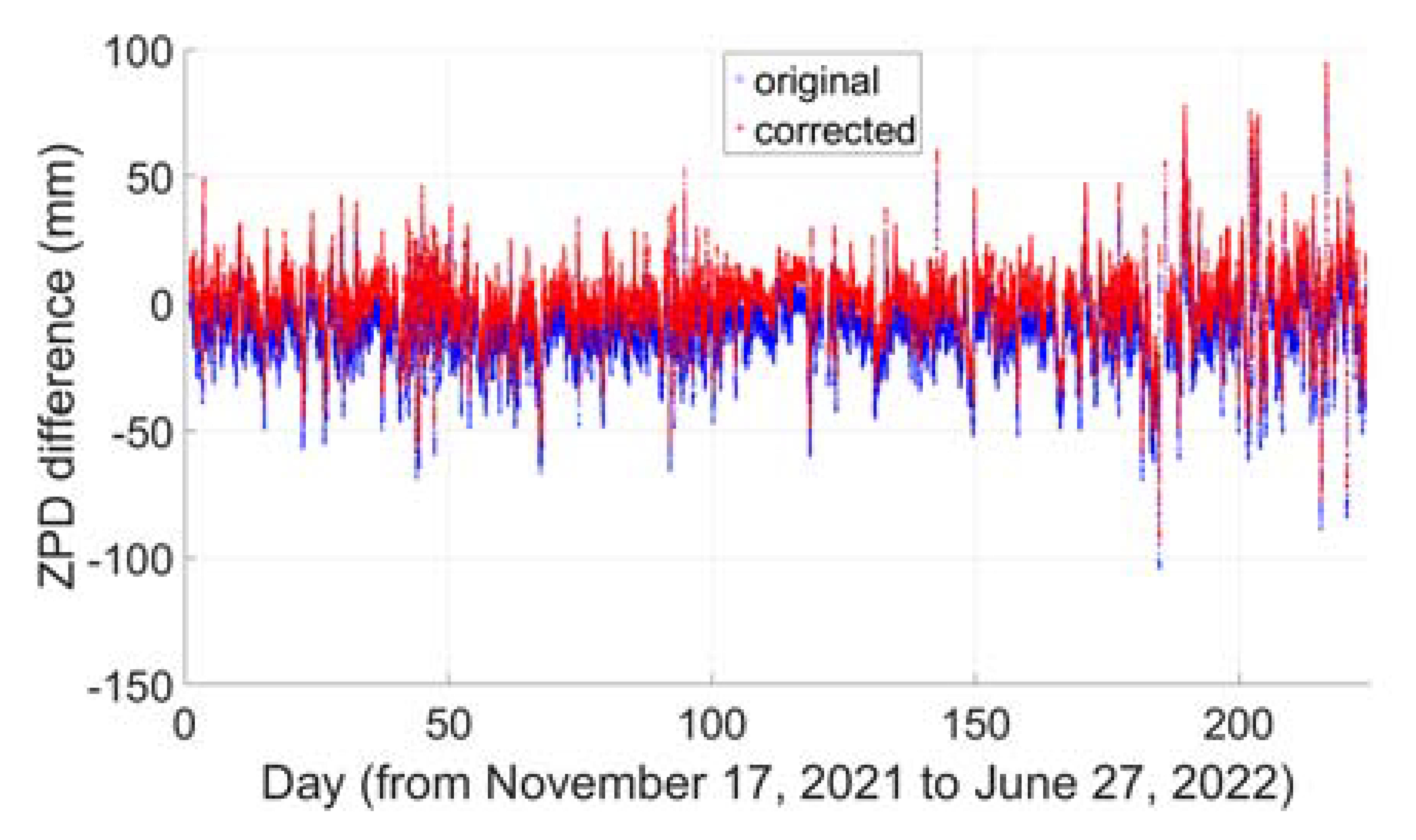
The detailed assessments are based on the baselines BRUX-REDU and BAUT-LEIJ. The distance between the two IGS stations BAUT (14.5°E, 51.2°N) and LEIJ (12.4°E, 51.3°N) is about 151 km and the receivers are both JAVAD TRE_3 DELTA. As the proposed method requires knowledge of the troposphere between these two stations,
Figure 12 and
Figure 13 show the differenced tropospheric zenith path delay (ZPD), based on IGS tropospheric products. For BRUX-REDU, it is from 1 January 2020 to 1 September 2021, while for BAUT-LEIJ, it is from 17 November 2021 to 27 June 2022. The blue values are the original values, while the red values are the values after correction with the Hopefield model. From the figures, we can see that after correction with the Hopefield model the ZPD difference between these two stations becomes much smaller; for BRUX-REDU, most of them are within 5 cm, and 99% are within 6 cm, and for BAUT-LEIJ, 99% are within 5 cm. The cases with ZPDs larger than 5 or 6 cm may be due to special weather conditions that need further research.
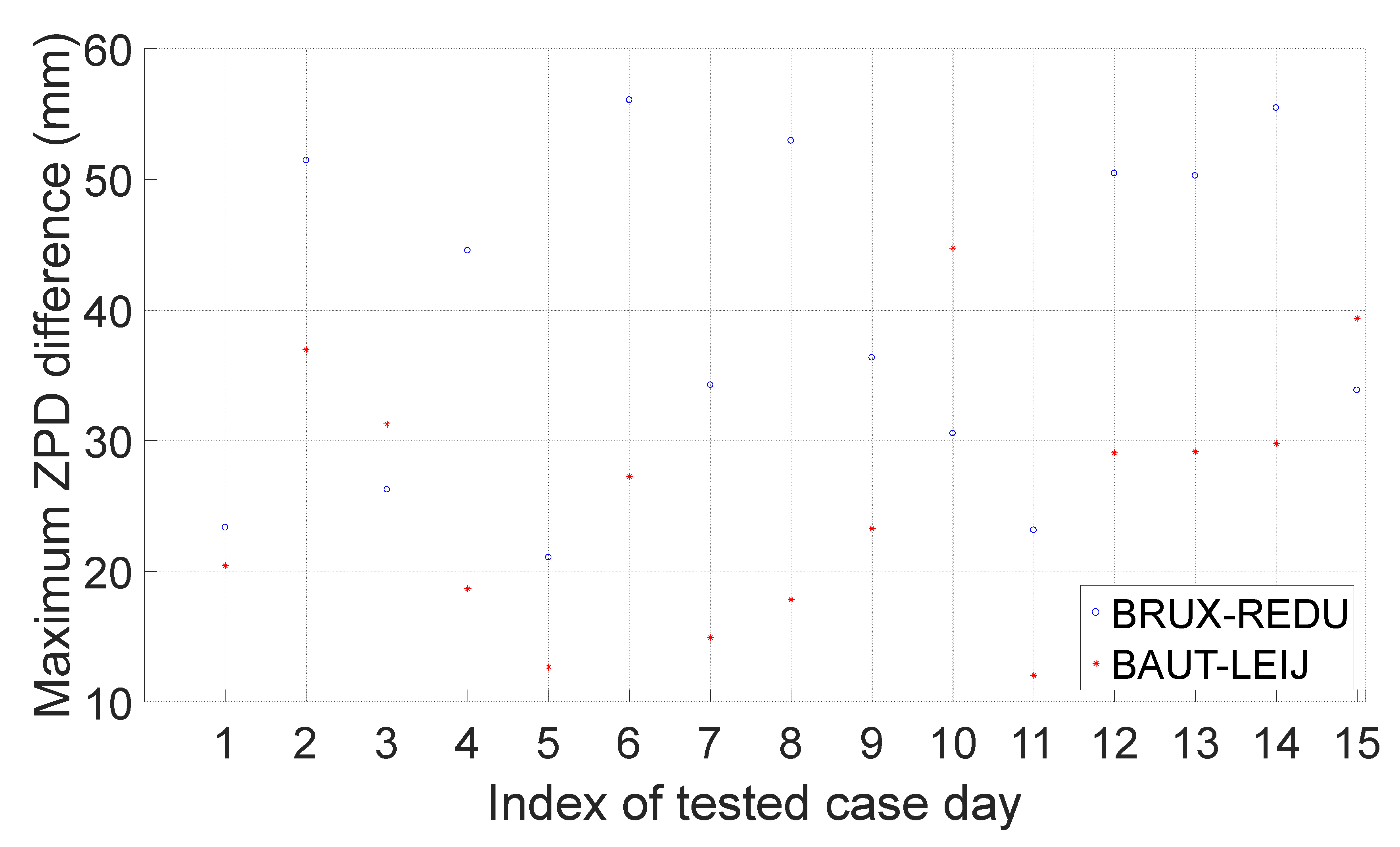
In this research, for BRUX-REDU, only observations of those days with a daily maximum differenced ZPD of no more than 6 cm will be used for assessment. As listed in
Table 12, fifteen-day observations in 2021 are randomly selected, and the days of the year are 1, 14, 32, 33, 60, 72, 91, 100, 121, 127, 152, 172, 182, 222 and 244. For BAUT-LEIJ, only observations of those days with a daily maximum differenced ZPD of no more than 5 cm will be used for assessment. The fifteen randomly selected days of 2022 are 1, 8, 14, 32, 33, 45, 60, 72, 94, 104, 122, 127, 152, 172 and 178. The maximum values of the daily differenced ZPD of these selected days are shown in
Figure 14 and range from about 1 cm to approximately 5.5 cm.
Figure 15,
Figure 16 and
Figure 17 show the performance of the extra-wide-lane ambiguity resolution for GPS, Galileo and BeiDou. Note that, since BeiDou carrier-phase type L7I is not available, only the extra-wide-lane ambiguity resolution of C56 and C12 is assessed. From these three figures, we can see that the ambiguity fixing rate of extra-wide lanes E57, E58, E78 and C12 can all reach 100%, and the fixing rate of G25 and E68 can reach more than 99%. Although the performance of C56 is the worst, it can also reach more than 96%.
Figure 18 and
Figure 19 show the wide-lane ambiguity resolution performance of N15 within the same GNSS and inter-GNSS. From
Figure 18, we can see that the ambiguity fixing rate of Galileo and BeiDou wide lanes C15 and E15 can reach approximately 98%, while that of GPS wide lane G15 is the smallest, but it can still reach more than 91%. From
Figure 19, we can see that the fixing rate of the inter-GNSS wide-lane ambiguity of N15 can reach more than 90%.
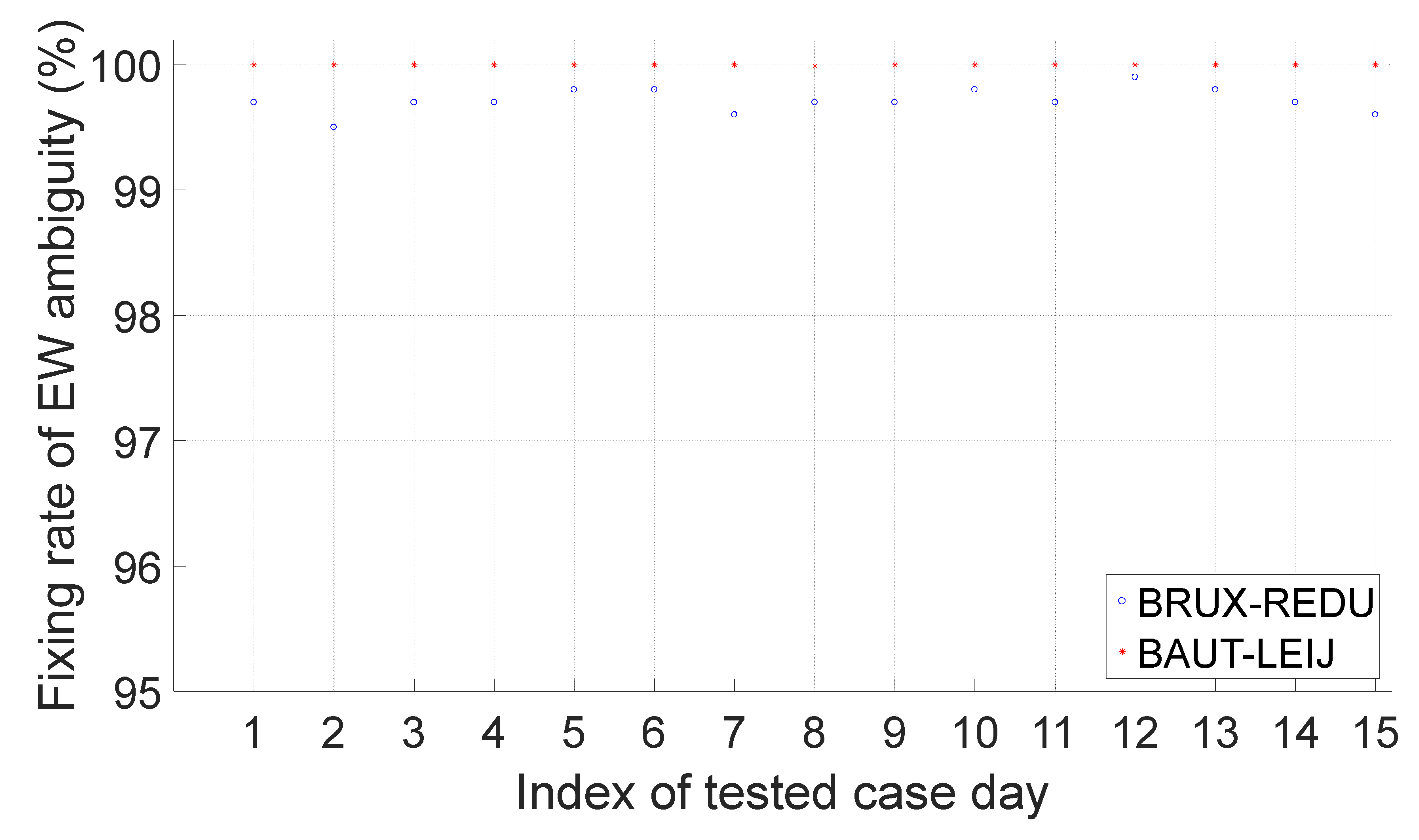
Figure 20 shows the narrow-lane ambiguity-resolution performance of all three GNSSs. We can see that the single-epoch fixing rate of BAUT-LEIJ can reach almost 100% and that of BRUX-REDU can reach approximately 95%. In addition, there is no misfixed case.
5. Conclusions
With multiple-frequency observations available, tropospheric delay has become the most important error source affecting CORS ambiguity resolution. In this research, taking advantage of shared carrier-phase types L1 and L5 of GPS, Galileo and BeiDou, we proposed a cascading ambiguity-resolution method that includes five ambiguity-resolution steps: extra-wide-lane ambiguity resolution, wide-lane ambiguity resolution, inter-GNSS wide-lane ambiguity resolution, a subset of narrow-lane ambiguity resolution, and other narrow-lane ambiguity resolutions. The best feature of the proposed method is that the tropospheric delay is neglected as much as possible while ensuring that it has no obvious effect on the ambiguity resolution:
For the ambiguity resolution of wide lanes within the same GNSS and inter-GNSS, the tropospheric delay is ignored directly, as simulated investigations show that it has no obvious effect, even with a size as large as 0.5 m.
For the ambiguity resolution of narrow lanes, a differencing scheme between satellites with similar wet mapping functions is proposed.
Based on the baselines formed between IGS stations BRUX and REDU, with a distance of approximately 104 km, and BAUT and LEIJ, with a distance of about 151 km, a detailed assessment is carried out. The numerical results show that the single-epoch ambiguity resolution can reach approximately 90%; therefore, we can say that single-epoch ambiguity resolution is feasible for a large-scale CORS network with a station distance as long as 100 km. In addition, as the method depends on the closeness between the wet mapping functions of different satellites, with more satellites the wet mapping functions will become closer. Therefore, in the near future, when all GPS satellites are modernized, the Galileo constellation is completed and all BeiDou-2 satellites become BeiDou-3, it is expected that the ambiguity-resolution performance will be further improved.
However, the proposed method has high requirements for receivers:
They should be multi-frequency and multi-GNSS and can observe satellites of GPS, Galileo and BeiDou.
They should have carrier phase types of both L1 and L5 for GPS, Galileo and BeiDou.
Additionally, the proposed method requires an understanding of the troposphere characteristics of the CORS network.


