Article

Data-Free Area Detection and Evaluation for Marine Satellite Data Products

1
College of Geodesy and Geomatics, Shandong University of Science and Technology, Qingdao 266590, China
2
College of Computer Science and Engineering, Shandong University of Science and Technology, Qingdao 266590, China
*
Author to whom correspondence should be addressed.
Remote Sens. 2022, 14(15), 3815; https://doi.org/10.3390/rs14153815
Submission received: 11 July 2022 / Revised: 1 August 2022 / Accepted: 4 August 2022 / Published: 8 August 2022
(This article belongs to the Section Ocean Remote Sensing)

Abstract

:
The uncertainty verification of satellite ocean color products and the bias analysis of multiple data are both indispensable in the evaluation of ocean color products. Incidentally, ocean color products often have missing information that causes the methods mentioned above to be difficult to evaluate these data effectively. We propose an analysis and evaluation method based on data-free area. The objective of this study is to evaluate the quality of ocean color products with respect to information integrity and continuity. First, we use an improved Spectral Angle Mapper, also called ISAM. It can automatically obtain the optimal threshold value for each class of objects. Then, based on ISAM, we perform spectral information mining on first-level Yellow Sea and Bohai Sea data obtained from the Geostationary Ocean Color Imager (GOCI), Moderate Resolution Imaging Spectroradiometer (MODIS) and Ocean and Land Color Instrument (OLCI). In this manner, quantitative results of information related to data-free areas of ocean data products are obtained. The findings indicate that the product data of OLCI are optimal with respect to both completeness and continuity. GOCI and MODIS have striking similarities in their quantitative or visualization results for both evaluation metrics. Moreover, a concomitant phenomenon of ocean-covered objects is apparent in the data-free area with temporal and spatial distribution characteristics. The two characteristics are subsequently explored for further analysis. The evaluation method adopted in this study can help to enrich the content of ocean color product evaluation, facilitate the research of cloud detection algorithms and further understand the composition of the data-free regional information of marine data products. The method proposed in this study has a wide application value.

Graphical Abstract

1. Introduction

The domestic and international research on ocean remote sensing has gradually intensified along with the free access of remote sensing data and the commissioning of ocean color satellites, including the Sea-viewing Wide Field-of-view Sensor (SeaWiFS), Moderate Resolution Imaging Spectroradiometer (MODIS), Geostationary Ocean Color Imager (GOCI) and Ocean and Land Color Instrument (OLCI). Various ocean and atmospheric parameter products can be inferred from spectrometer signals measured by dedicated atmospherically corrected space-borne ocean color sensor data and related in-water bio-optical algorithms [1]. However, the extensiveness of ocean color information relies on the inversion of an extremely small number of signals [2,3]. Most signals received by ocean color satellites (e.g., atmospheric signals) are noisy, and only 10% are oceanic signals. Other problems include cloud occlusion, sensor failure or noise that hinders the acquisition of ocean color information [4,5]. For example, 15 of the 20 detectors in band 6 of the Aqua MODIS are invalid. The sensor sometimes fails to generate meaningful results, even obtaining random error results due to missing pixels called dead pixels [6]. In more complex sea conditions, cloud masking or other denoising steps are necessary. Furthermore, depending on the choice of the cloud detection algorithm and denoising algorithm that vary with respect to capabilities or sizes, some normal image pixels are treated as clouds or masked pixels. Therefore, the ocean color data of a region of interest tend to have a high missing rate or even a complete missing result. The estuary of the Yangtze River has high sediment turbid waters, green tide algae disasters in summer and heavy eutrophication or areas with a highly suspended solid concentration [2]. In this area, cloud pixels are difficult to isolate from the high sediment and phytoplankton content, because the sea areas have an even higher reflectance compared with the clear water in the near-infrared band [7]. Such a situation may cause the loss of normal ocean color information. As a result, the ocean color products show a missing state at a certain spatial location, also called a data-free area. The existence of data-free areas seriously affects the spatial and temporal continuity of the information of the product data, reduces the value of data products and causes a great obstacle to the research of oceans.
The quantification of uncertainties and quality aspects of satellite ocean color products is one of the central tasks of ocean color missions [8,9]. From a satellite operation perspective, most of the validation and quality assessments of ocean color products are performed for individual or specific missions [10,11,12]. Image quality assessment methods usually include both subjective and objective evaluations. Experienced scientists usually perform subjective evaluations under the guidance of a complete scientific evaluation procedure for graphics [13]. By contrast, objective evaluation is based on the objective characteristics of images, and relevant rigorous mathematical models are adopted to evaluate the images and obtain evaluation results that are extremely close to human vision [14]. Objective evaluations can be divided into full-reference, weak-reference and no-reference image quality evaluations depending on the presence or absence of reference image information [15]. A full-reference image quality evaluation initially obtains a high-quality scene as a standard image and then compares the features with the image to be measured, and finally, certain similarities in the commonly used feature parameters (e.g., mean square error and peak signal-to-noise ratio) are calculated [16]. Sherkh et al. [17] proposed the information fidelity criterion based on the mutual information approach. Shannon [18,19] implemented a reference-free image quality evaluation and used the grayscale mean gradient, image signal-to-noise ratio, and the information entropy metric to evaluate the quality of an image to be measured under the condition of a missing standard image. Zhu et al. [20] designed a watermarking algorithm based on motion blur degradation/restoration. There are also some classical algorithms, such as the semi-referential Special Sensor Microwave/Imager methods and VIF methods [21,22,23]. In the aforementioned methods, only a part of the feature information of the standard images is used as the basis for evaluation, and only low-quality standard images are considered. Furthermore, the aforementioned methods obtain data that are closer to human visual perception compared with those requiring image quality evaluation but that lack a reference image, which is also called a weak reference image quality evaluation. In this study, Level 1 data are used as the reference data, and Level 2 ocean color product data are used as the image for evaluation. Then, a robust weak reference method is used to mine the spectral information of the data-free area. Some of the non-reference indicators are also used to evaluate the information of the products.
The acquisition of the ocean color information of highly turbid areas of the ocean has been a challenge for ocean color remote sensing researchers [24,25,26,27]. The reasons for the absence of information to form a data-free area, the main types of marine objects contained in the data-free area and the spatial and temporal distribution characteristics exhibited by the absence are the central concerns of ocean color research. Traditionally, uncertainty and quality evaluations of ocean color products are based on field measurement data values that are used as the veracity-check or multi-sensor product values in deviation analysis [28,29,30,31,32]. Incidentally, high-quality standard images or actual measurement data are difficult to obtain. The content of ocean color product quality evaluation needs to be enriched. This study aims to investigate the evaluation of remotely sensed ocean color products from another perspective. We propose a method for the analysis and evaluation of Marine products based on regions with no data. The spectral information mining of Level 1 data is employed to achieve the following objectives: (1) to study the types of marine coverage objects contained in the data-free areas of remote sensing ocean color products in the Yellow Sea and the Bohai Sea; (2) to determine the presence or absence of temporal and spatial distribution characteristics of the missing information that correspond to the types of marine objects; (3) to conduct a correlation analysis of the missing temporal and spatial distribution characteristics of the different ocean color satellite data (GOCI, MODIS and OLCI); and (4) to analyze and evaluate the data based on two indicators, namely, data integrity and the continuity of ocean color information. In summary, we evaluated the missing pixels during the quality marking of the products. Moreover, the object of the study remains as the ocean color product itself, which we analyzed and evaluated in detail for both subjectivity and objectivity. This study is expected to enhance the scientific knowledge of data-free areas of ocean color data. It provides scientific and theoretical support to producers and users of the products and ensures the reliability of subsequent research and applications. Furthermore, this study explores the origin of the spatial and temporal patterns of the data-free areas and subsequently attempts to explain the related characteristic phenomena. We expect the detection and evaluation of ocean color products of data-free areas to help improve atmospheric correction algorithms, optimize cloud detection algorithms, reconstruct missing data, achieve evaluations of different satellite products, and enhance the application of the feature mining of data-free areas. New methods are provided for researchers to study data-free areas of marine products.

2. Materials and Methods

2.1. Study Area

The areas selected for this study are the Yellow Sea and the Bohai Sea of China (32° to 41°, 117° to 126°; Figure 1). The Bohai Sea is the northernmost offshore sea of China and the internal sea of the People’s Republic of China. It is surrounded by land on three sides, with Liaoning Province to the north, Tianjin City and Hebei Province to the west and Shandong Province to the south. The eastern side is divided from the Yellow Sea by a joint line from the old Tieshan Cape on the Liaodong Peninsula through Miao Island to the Penglai cape at the northern end of the Shandong Peninsula. Moreover, the Yellow Sea is located between China and the Korean Peninsula. It is the largest marginal sea in the western part of the Pacific Ocean, and it is connected to the Bohai Sea through the Bohai Strait. Both seas cover an area of approximately 460,000 square kilometers and are rich in marine biological resources, making them an important part of China’s marine economy [33].

2.2. Date Collection

2.2.1. GOCI, MODIS and OLCI L-1 Data

Korea successfully launched the world’s first geostationary ocean color satellite called Communication Ocean and Meteorological Satellite (COMS) on 26 June 2010. The GOCI on top of COMS has eight bands with a range of 0.4–0.9 μm and a spatial resolution of 500 m. COMS has a high temporal resolution and can generate eight remote sensing images from 8:00 a.m. to 3:00 p.m. (Beijing time) every day at time intervals of 1 h. Ocean color data can be obtained at the regional scale for the East Asian seas around the Korean Peninsula [34], and their high temporal resolution is exceptional for ocean color monitoring [35]. In this study, we selected COMS_GOCI_L1B and COMS_GOCI_L2A as the research data. COMS_GOCI_L1B, with its complete information, was used as the primary data without calibration and spatial correction processing. By contrast, COMS_GOCI_L2A, which includes the data-free area, was used as the secondary ocean color product data, as provided by GOCI.
MODIS, the most important sensor in the U.S. Earth Observation System, was successfully launched on 4 May 2002, onboard the two satellites of Terra and Aqua. Its 36 bands range from 0.4 to 14.38 μm, with a spatial resolution of 250/500/1000 m and a temporal resolution of 1 day. Owing to the excellent imaging capability and early public time of MODIS, its data are widely used in research in various industries [36,37,38]. Among them, MOD02KM is the Level 1 data, with a spatial resolution of 1000 m and complete information. Moreover, L2_LAC_OC is the full-resolution ocean color product data with local area coverage.
The OLCI onboard the Sentinel 3 satellite was launched on 16 February 2016. Its 21 bands ranging from 0.4 to 1.02 μm, with a spatial resolution of 300 m and a temporal resolution of 2 days. The excellent spatial and temporal resolution and relatively good spectral resolution of OLCI have gradually been accepted by the public, and an increasing number of researchers have scientifically processed the OLCI data [39,40,41]. Here, the selected datasets were OL_1_EFR and OL_2_WFR. OL_1_EFR is the uncalibrated full-resolution atmospheric radiation with complete information, whereas OL_2_WFR is the full-resolution ocean color product with the data-free area. Table 1 summarizes the data used in the study and the corresponding information.

2.2.2. GOCI, MODIS and OLCI Products

The Yellow Sea and Bohai Sea are often covered by clouds, and only a few clear and reliable pixels can be collected in the range of interest. This means that there are serious limitations in collecting various information for all seasons and different atmospheric states [42]. A statistical analysis of the missing data of the Yellow Sea and Bohai Sea over the years have found that green tide algae outbreaks were frequent in 2019. The coastal eutrophication was serious, and the marine ecological environment was complex. These conditions render the data-free area significantly more representative.
We selected standard spectral samples in June (in the period of green tide outbreak and more serious coastal pollution) and January (in the period of sea ice outbreak). Moreover, we adopted the images of 23 June 2019 and 20 January 2019, with less cloudiness, and used them as the standard images for selecting the spectral samples. In this manner, the temporal phase of the data could be unified, and the effect of green tide algae and cloud movement could be reduced.
Consequently, we selected a total of 33 views of GOCI, MODIS and OLCI image data of the Yellow Sea and Bohai Sea taken in all seasons of 2019 (i.e., two views per sensor data in winter and three views per sensor data for each of the other seasons). The selected data included Level 1 data without calibration processing and Level 2 product data with data-free areas under the same spatiotemporal conditions (Table 2). The data-free area is present in the vast majority of the product data for the same sensor, and it is spatially located in the same place. Here, the Level 2 product data were only used to determine the spatial location of the data-free area and the size of the area. Consequently, the chlorophyll concentration product, which is commonly used in ocean color products, was selected as the image data for evaluation.

2.3. Methods

The framework and technical approach of this study are described in Figure 2. The specific pre-processing process and methods for the Level 1 and Level 2 data are described in Section 2.3.1 and Section 2.3.2. The improved method of the automatic acquisition of the optimal thresholds of the SAM algorithm as applied to the marine object recognition and classification in this study is presented in Section 2.3.3. The corresponding product analysis and evaluation index calculation methods and the results are described in Section 3.

2.3.1. Data Pre-Processing

The Level 1 data of GOCI, MODIS and OLCI were pre-processed to obtain the remotely sensed water reflectance ( ρ w ) of the images after radiometric calibration, atmospheric correction, geometric correction and sea–land separation. The spectral curves of the sample library should be standardized to be able to fit the other post-processing processes of the remote sensing images. Thus, the reflectance of water ( ρ w ) was converted into remote sensing reflectance ( R r s ). In ocean remote sensing, ρ w   =   ρ f [43]. By neglecting the optical thickness of gaseous aerosols, such as ozone and water vapor [44], τ = 0. The remote sensing reflectance ( R r s ) can be obtained as follows:
R r s = ρ w π τ 0 ,
τ 0 = exp ( τ cos θ 0 / 2 ) ,
where τ 0 is the diffuse transmission ratio, τ is the aerosol optical thickness and θ 0 is the solar zenith angle.
Level 2 data were geometrically corrected to convert the data-free area into vector data. The R r s image obtained using Equation (1) was cropped to obtain the R r s image data corresponding to the spatial location of the data-free area only.
The wave spectral data of the data-free area showed that the ocean coverage objects at the spatial location of the data-free area were mostly composed of clean water, turbid water, green tide algae, clouds and sea ice. Thus, the five marine coverage types that are most common in the ocean and that may have an impact on the missing data were selected as the targets of this study. The spectral differences between the categories of the five marine coverage objects were large. Consequently, Spectral Angle Mapper Classification (SAM) was chosen as the identification classification method. The correctness of the standard spectral curve, which is the core of the algorithm, was particularly important in the study.
The traditional endmember extraction methods, such as the pixel purity index (PPI, i.e., based on the principle of convex geometry). The basic principle is to form a single-row body in the feature space, with its endmembers located at the vertices of the single-row body [45]. In practical applications, an MNF dimensionality reduction transformation is usually performed on the data before the endmembers are extracted using PPI. Then, the result is integrated into an N-dimensional visualization window for endmember extraction. However, this method is mainly applicable to hyperspectral data. It is also a supervised algorithm with many steps, suggesting a complex process, and it entails high subjectivity [46]. As the spectral resolution of the multispectral data is already much lower than that of hyperspectral data and because its band information is less, the information is no longer suitable for dimensionality reduction processing. Moreover, the dimensionality reduction transformation of MNF does not apply to multispectral data. Therefore, in this study, we separately extracted the endmembers to determine the corresponding spatial locations before selecting the spectral library samples. Then, the standard spectral data obtained by the method were identified and classified by their higher accuracy and better robustness.

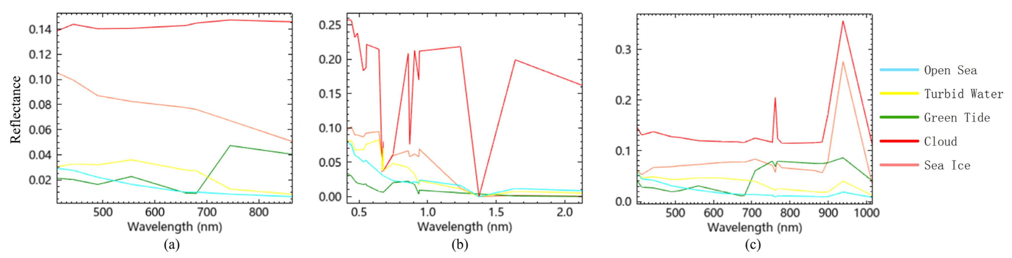
2.3.2. Acquisition of Endmembers Spectral Data

  • Endmember of Green Tide Algae
The normalized difference vegetation index (NDVI), a green tide extraction algorithm, is widely used because of its reliable and robust performance [47].
N D V I = N I R R N I R + R ,
where NIR is the reflectance of the near-infrared band, and R is the reflectance of the red band.
The theoretical value of threshold T is 0 but fluctuates due to factors such as shallowness and water depth [48]. The threshold T of NDVI was determined by visually interpreting the threshold segmentation and false-color images of NDVI in order to eliminate the influence of thin clouds and coastal waters and to unify the conditions. After many experiments, the threshold was determined to be [−0.05, 0.80]. The results are shown in Figure 3.
2.
Endmember of Clouds
The apparent atmospheric reflectance images in the R, G and B bands after radiometric calibration were processed and converted into images with distinct cloud features [49]. Then, cloud detection was performed on the cloud feature images. This method could greatly improve the detection accuracy of clouds compared with the general threshold method of cloud detection. The specific process is shown in Figure 4.
The equation for converting the RGB image into a cloud feature image with specific coefficients is given by
G r a y = P M ,
P = [ 0.229 0.587 0.114 0.595716 0.274453 0.321263 0.211456 0.522591 0.311135 ]       M = [ R G B ] ,
where P is the specific coefficient converted to a grayscale image with prominent cloud features [50], and R, G and B are the reflectance of the red, green and blue light bands, respectively. The cloud detection results are shown in Figure 5.
3.
Endmember of Turbid Water, Clean Water and Sea Ice
The spatial locations of turbid water, clean water and sea ice were selected based on the schematic diagram of the distribution of water quality conditions in China’s jurisdictional waters, as reported in the 2019 Bulletin of the State of China’s Marine Ecological Environment of the China Marine Information Network (http://www.nmdis.org.cn/, accessed on 20 June 2021).
For the spatial locations of the five types of marine objects in the study area, 100 samples of the corresponding endmember spectral information were selected. The endmember spectral curve information of each type of marine object was obtained by Equation (6). Then, the average spectral information of each type of marine object was obtained by Equation (7). The calculated results were adopted as the standard spectral curve information and were saved as a binary data file (.sli) for establishing the spectral library of the five types of marine objects (Figure 6).

2.3.3. Optimal Threshold Automatic Acquisition via the Improved SAM (ISAM) Algorithm

The SAM [50] was chosen as the recognition classification method in this study. It is a method based on vector space and spectral shape analysis. It is suitable for the image recognition and classification of the overall similarity of spectral shapes of marine coverage objects [51]. In SAM, the spectral data appear as vectors in multidimensional space, and the angle between the spectrum of a pixel and the standard spectral vector of a sample is determined by employing a corresponding computational equation (Figure 7). Furthermore, a suitable angle threshold is set. If the angles between two spectral vectors are less than the threshold, they are classified as a single category in feature identification.
The equation for calculating the angle between the spectra is expressed as follows:
θ = cos 1 T · R | | T | | · | | R | | = cos 1 i = 1 n t i · r i i = 1 n t i 2 i = 1 n r i 2 ,
where θ is the angle representing the similarity between the different spectra. As the θ becomes smaller, the similarities between the two spectra become greater, and as the θ becomes larger, the difference becomes greater. T( t 1 , t 2 t n ) is the sample spectral library spectrum of the n bands, and R( r 1 , r 2 r n ) is the data of the spectra to be classified. When M( T 1 , T 2 T m ) sample points are selected as the spectral library spectra in an image class, the class center is used as the geometric mean vector of the selected spectra in the region.
T ¯ = 1 M 1 M T i ,
The angle θ threshold (0−π/2) of the two spectral vectors in the SAM algorithm is particularly critical. The accuracy of recognition classification is affected by either an extremely large threshold or an extremely small threshold. When the threshold is extremely large, misclassifications occur. When the threshold is extremely small, some data are unclassified. Only an appropriate threshold can increase the rigor of the classification results. Therefore, this study improves the SAM, also called ISAM, algorithm to automatically obtain the most suitable threshold value, reduce the subjective influence of human intervention and increase the objectivity of the classification results.
The specific improvement measures are based on the SAM algorithm. First, we evenly selected 100 training samples for each class of ocean objects and removed half of the samples in the data-free areas of the Level 2 product data from the training samples, and we used them as validation samples. The reason for selecting half of the samples and using them as validation samples was that all of the cloud pixels were present in the data-free area. Then, each class of marine coverage type objects is given an initial angle threshold. It is iteratively calculated using the overall accuracy of the classification as the judgment criterion. Different iteration steps can be artificially set to adjust the time complexity of the algorithm, allowing for the obtainment of the angular threshold results for each class of classified objects. The initial angle of each type of object is set to 0.05 radians (R), and the iteration step size is selected to be 0.005. There were threshold interactions between object classes and differences in pixel size between data. This resulted in different classification thresholds for each object between different data sets (Table 3). The impact of the difference in spatial resolution between the data on the classification results is analyzed in depth in the subsequent discussion section. The obtained angular thresholds are theoretically applicable to all data under the same sensor. It improves the efficiency of the subsequent identification of a large number of data.
As the SAM classification method is pixel-based, the spectral vectors are calculated pixel by pixel, and the recognition classification results are usually fragmented (Figure 8a). In this study, high-pass filtering was performed on the SAM recognition classification results to enhance the texture information, followed by Clump clustering [52]. By using the mathematical morphology operator, the classification results with the enhanced texture information can be clustered and merged with the adjacent fragmented but similar classification regions. After the initial classification, the individually classified pixels can be merged by the ISAM method. This improves spatial continuity and classification accuracy. The improved classification result is shown in Figure 8b.
The comparative classification results clearly show that the images were fragmented before the processing of the Clump algorithm (Figure 8a). The number of pixels in a separate category is high and does not correspond to the actual situation. By contrast, Figure 8b shows that some fragmented similarity areas (patches) can be combined to achieve good spatial continuity.

3. Results

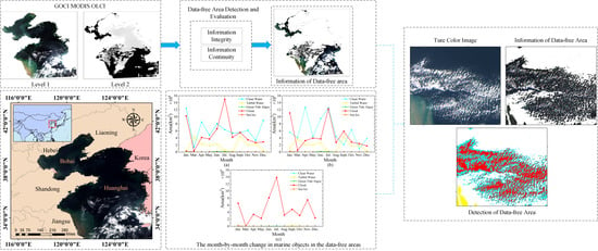
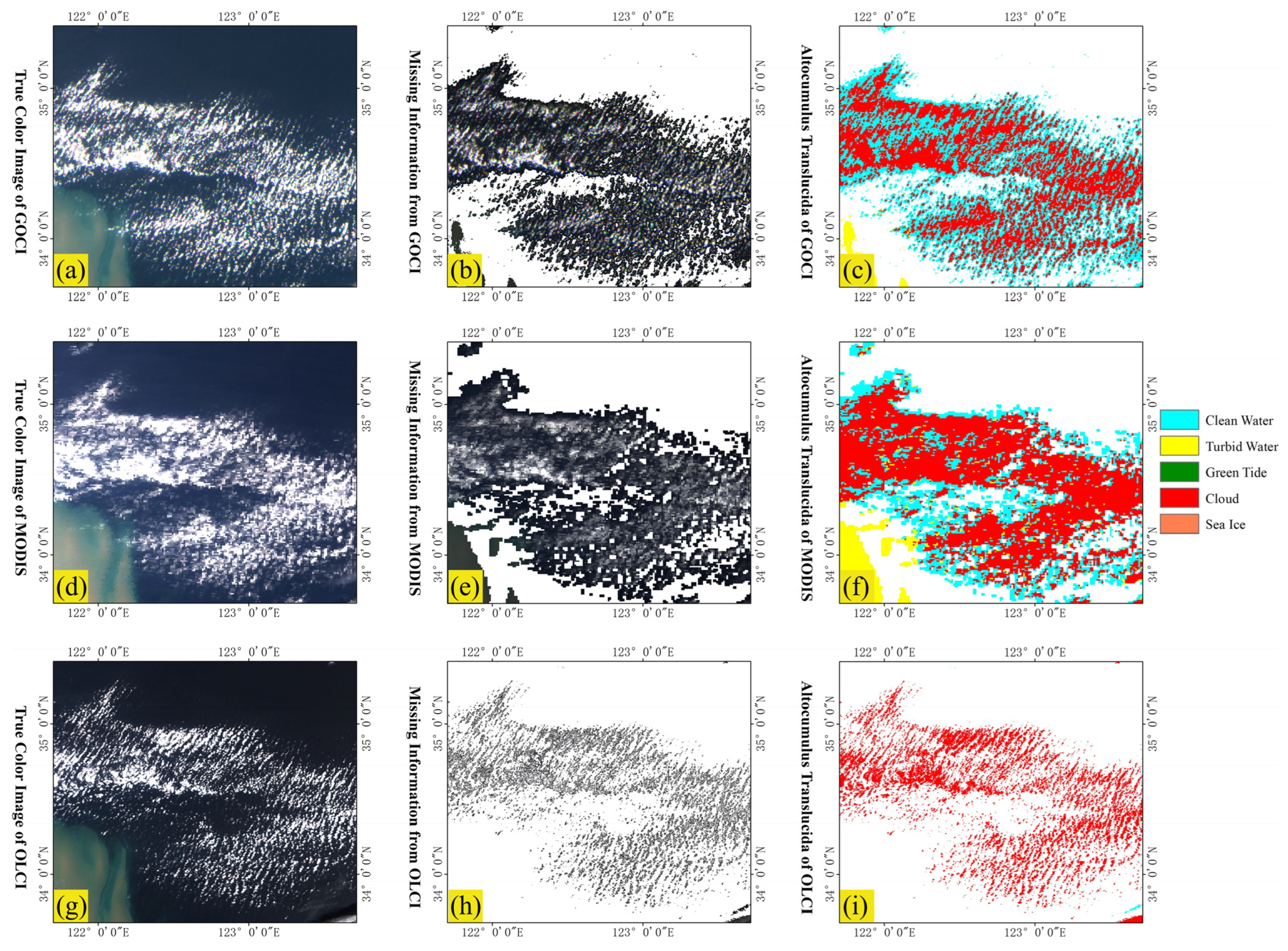
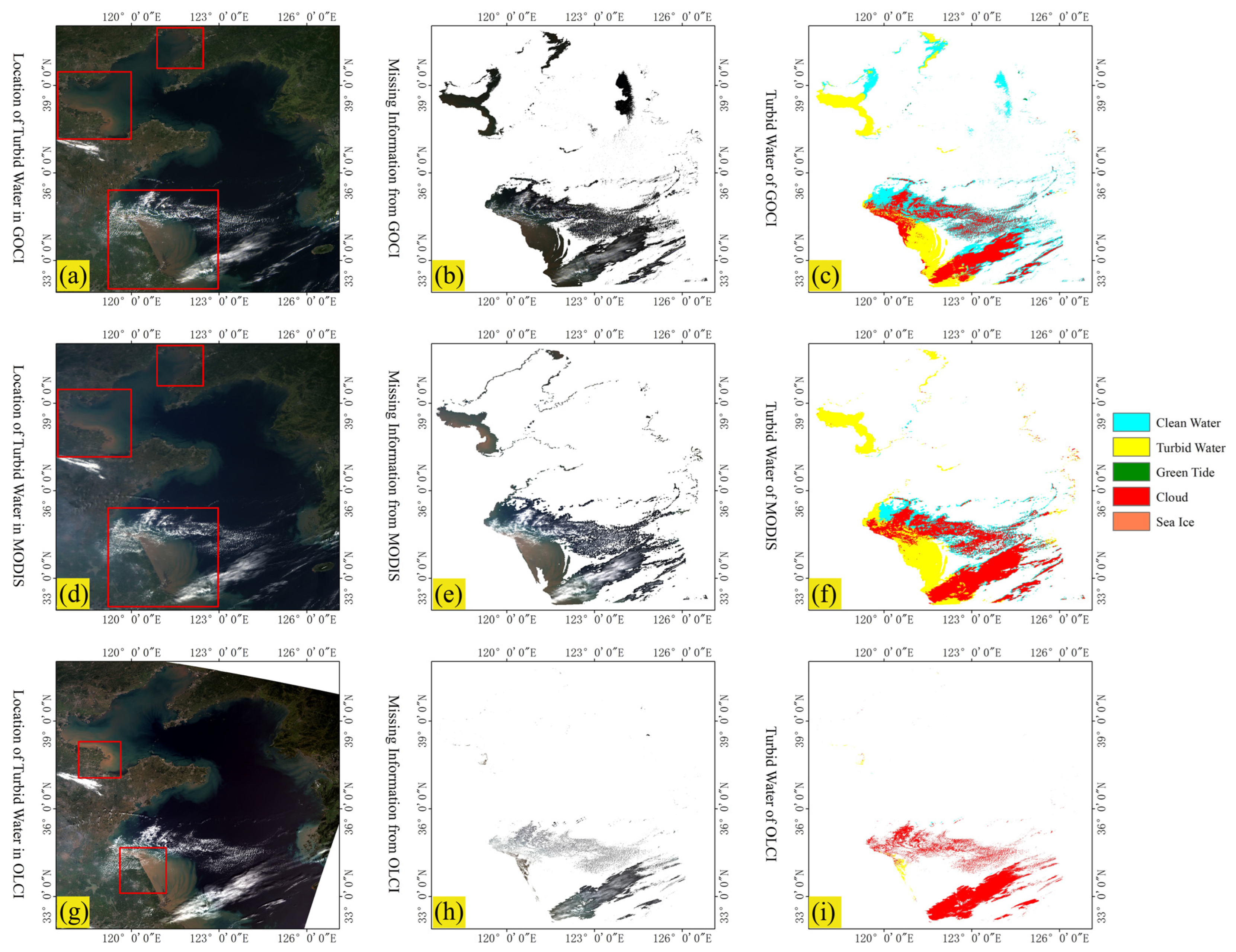
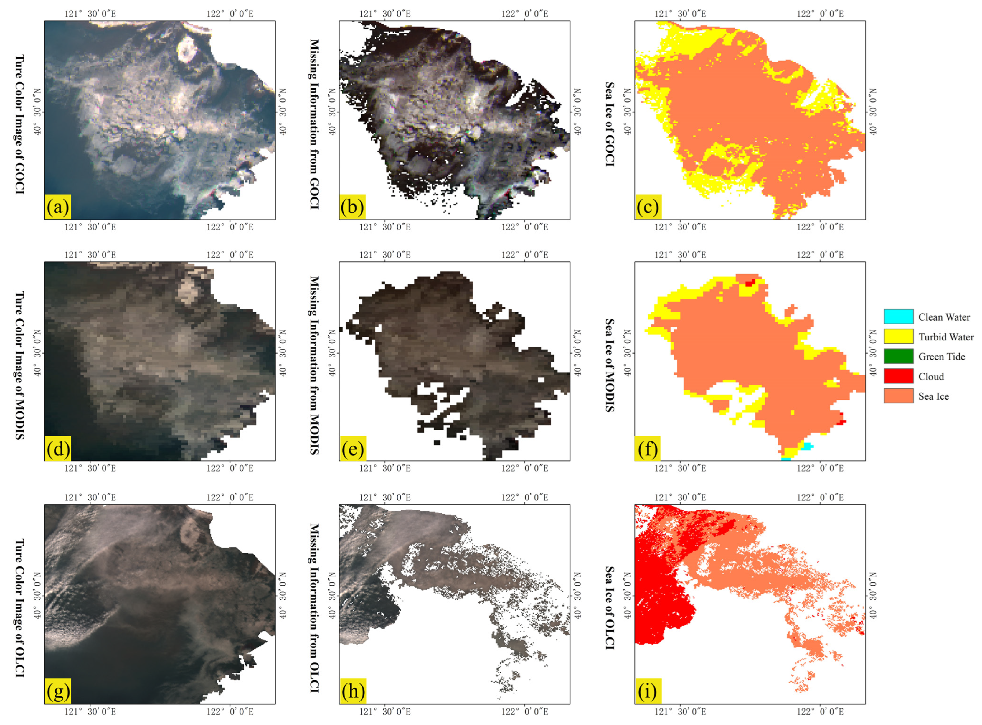
3.1. Detection of Data-Free Area

The confusion matrix was constructed using the validation sample set. Then, the obtained overall accuracy, Kappa coefficient, production accuracy and user accuracy were used to evaluate the accuracy of the classification results (i.e., the mean value of the classification results for each of the 11 scenes). The Kappa coefficient forms a complementary relationship with the overall accuracy [53].
As shown in Table 4, the user accuracy of the results for all three sensor data is greater than 90%. The lowest Kappa coefficient is 0.86 for MODIS. Moreover, the lowest overall accuracy is 89.3% for MODIS, whereas the highest is 95.7 for OLCI. The obtained classification results have good accuracy. On the one hand, the separate extraction of the endmember data can eliminate the effect of the mixed pixel background for standard spectral data. On the other hand, the clustering process of the Clump algorithm can eliminate fragmentation while increasing the spatial continuity of the classification results, thus improving the classification accuracy. The accuracy of the results from using ISAM in this research is higher compared with the results of other studies that used SAM algorithms [54,55].

3.2. Data Product Analysis and Evaluation

3.2.1. Integrity of Ocean Color Information

The ecological environments of marine areas are complex, and remote sensing products with missing information are common in this case. Cloud occlusion is the main factor in the low spatial continuity of product data [56,57,58]. Moreover, the differences in algorithms for cloud detection or noise removal processes may result in missing normal pixels of the data product, thus greatly increasing the missing rate of the product. In this study, this loss of ocean color information corresponding to cloud-free pixels is called abnormal missing information. Table 5 shows the main types of marine coverage compositions and their area statues in the product data-free areas. The area and missing rate are calculated as follows.
A i = S i · R i 2 ,
L i = 1 n A i S · 100 % ,
where S i (n = 3) represents the number of image elements of each category in the recognition classification result, S is the total area size of the area of interest in a single view, R i is the resolution size of a remote sensing image of GOCI (0.5 km), MODIS (1 km) and OLCI (0.3 km), A i is the area size of each category and L i is the missing rate of each image.
As shown in Table 5 and Figure 9, the missing rate of GOCI is mainly in the range of 15% to 30%, whereas that of MODIS is mainly in the range of 15% to 35%, with a large variation in missing rate per month. The missing rate of OLCI is mainly in the range of 4% to 15%, with less variation in the size of the missing rate per month. Its information is more complete and robust than those of GOCI and MODIS. Interestingly, the missing rates of the three products for January, June and July are larger than in the other months. MODIS products even lost half of their information in July. In addition, not only are the trends of the missing rates similar among the three products, but the monthly magnitudes of the missing rates of GOCI and MODIS are similar.
With respect to the completeness of data, the information was judged based on the average annual missing rate indicator only. The quality of OLCI is better than the other two product data, followed by that of GOCI, whereas MODIS has the lowest quality. However, the three data missing rates are large, and the monthly missing rates of GOCI and MODIS products are similar to the inter-annual variations. The remote sensing information corresponding to the spatial location of Level 1 data in the product data-free area is complex. A single missing rate indicator cannot accurately describe the quality of the GOCI and MODIS products. Therefore, the remote sensing information of the products’ data-free areas was mined to further obtain the missing information and improve the quality evaluation of the ocean color products. Level 1 data were mined for spectral information by using ISAM. The composition and distribution of the main marine objects in the product data-free area are shown in Table 6.
Table 6 particularly shows the total annual areas of the five common marine coverage objects in the product data-free area and their proportions. For GOCI and MODIS, the largest proportions of marine coverage objects in the data-free area are the clean water areas in the open ocean (both at approximately 47.7%), followed by those with cloud pixels (approximately 37.5%) of the data-free area. The difference between the two products and the OLCI product can be attributed to the presence of cloud pixels occupying 98.885% of the data-free area. Presumably, the composition of ocean-covered objects in the data-free area of OLCI was primarily clouds, a phenomenon that is consistent with the actual situation.
The areas of each type of marine coverage object in the GOCI and MODIS data-free areas showed a concomitant increase or decrease (Figure 10). The trend indicates that the data are similar not only in their total missing rate but also in the missing rate of each type of marine object.
The remote sensing information on the spatial locations of cloud pixels is inevitably lost after cloud detection and the cloud mask pre-processing of remote sensing data. Different satellites can hardly obtain data at the same time because of their respective but varying sensor imaging mechanisms and revisit cycles. Furthermore, cloud drifts are unavoidable. Clouds at the edges of an area disappear from the range of interest because of their movement, thus affecting the size of the data-free area. Here, we attempted to remove the cloud pixels in the ocean coverage type of the data-free area and evaluate the quality of the products by using the abnormal missing indicator as a means of reducing the statistical error caused by cloud movement. It is shown in the second sub-column of the percentages in Table 6.
As shown in Figure 6, the clean water of GOCI and MODIS has the largest proportion of anomalously missing information, even reaching 77%. The anomalous missing information of GOCI and MODIS are also extremely similar. However, the result of OLCI is extremely different, with an anomalous missing ratio of only 1.115% (i.e., the area is 6223.77 km 2 ). It is less than 1% of the missing areas of the other two products. The main type of deficiency is turbid water, accounting for 40.762%, followed by clean water at 27.044%.
The total percentage and total area of the anomalous missing data in the data-free area of GOCI and MODIS are much larger than the value of the anomalous missing data in the data-free areas of OLCI. Figure 11 shows the line graphs of the monthly abnormal missing area and abnormal missing rate. OLCI has the lowest abnormal missing ocean color information and the highest stable performance with respect to continuity in time patterns. The anomalous missing information of GOCI and MODIS ocean color information is higher than 30%, and the amount of missing data fluctuates greatly. Both have an abnormal missing rate exceeding 90% on March 13, and the information integrity is extremely low.
The above findings indicate that OLCI is superior with respect to the completeness of ocean color information and the continuity of the missing time distribution, followed by GOCI, whereas the lowest performance is for MODIS.
Turbid water, green tide algae and sea ice have reflectance magnitudes similar to that of clouds in the near-infrared band. This results in the cloud mask algorithm being much less capable of handling these types of marine coverage objects, particularly in the data-free area in this study. However, the proportion of clean water, as normal remote sensing information, is the largest for GOCI and MODIS, both with respect to all ocean coverage object types and anomalous missing information. The data-free area statuses of GOCI and MODIS have a high similarity, and this aspect is further analyzed in the following discussion.

3.2.2. Continuity of Ocean Color Information

The year-round presence of clouds over the ocean leads to the inevitable existence of data-free areas in ocean color products [4]. Given this circumstance, users often focus on the quality of the continuity of product ocean color information in the spatial and temporal patterns, i.e., the discrete problem of the data-free areas of the products [59,60]. Our findings indicate that a single missing rate indicator cannot sufficiently reflect the overall quality status of products, and it is only applicable to the quality assessment of single-view images. In other words, the existing quality evaluation method is highly restrictive, and it presents certain limitations in visually describing the quality status of products to be unified in time and space. Thus, we attempted to find a suitable indicator for describing the quality condition of the continuity of the product as a whole, which can also be called the missing spatiotemporal dispersion indicator.
The data containing the spatiotemporal information of data-free areas should be initially obtained prior to the calculation of the missing spatiotemporal dispersion indicators. In this study, we further attempted to fuse the missing information of each product with temporal and spatial data into a single scene image to be able to obtain the corresponding index parameters. First, the data-free area information is binarized (0 for data-free area; 1 for data-available area). Then, the spatiotemporal image results of the inter-annual data-free area of a corresponding product are calculated as follows:
M = { 1     ( D a t a f r e e   a r e a ) 0                           ( O t h e r   a r e a s ) ,
I = 1 n M i M m a x M m i n ,
where M is the result of the binarization of each view image, and I is the spatiotemporal image of the data-free area. The results are shown in Figure 12.
The spatiotemporal image obtained via calculation can visually depict the main distribution of the data-free areas in the Yellow Sea and Bohai Sea. GOCI and MODIS have high missing amount percentages for Bohai Bay, Laizhou Bay, Liaodong Bay of the Bohai Sea and the Yangtze River Delta of the Yellow Sea. Furthermore, GOCI was completely missing information in the Yangtze River Delta. The obtained results suggest that the data-free areas in these regions are mostly composed of turbid water near the shore. For example, the missing location of OLCI is usually in the middle of the sea, as opposed to the other two types of data, OLCI is missing to a lesser extent on the nearshore. The missingness is mostly due to the influence of clouds. The above method of directly evaluating the spatiotemporal distribution of data-free areas is called subjective evaluation, which is a common evaluation method in the field of remote sensing. This method is convenient and intuitive but susceptible to the influence of subjective factors, and the obtained results are not comprehensive and cannot unify the evaluation standards [61]. In ensuring that the evaluation of the three kinds of data is objective, quantified indicators are selected to correlate the spatiotemporal dispersion of the data in this study.
Standard deviation reflects the degree of dispersion of a dataset. A large standard deviation represents a large degree of dispersion of the data in the dataset. The standard deviation of the spatiotemporal image map constructed in this study reflects the dispersion degree of the data-free area. As the standard deviation becomes larger, the spatiotemporal dispersion of an image becomes stronger. As shown in Table 7, the spatiotemporal dispersion of the data-free area in OLCI is better than those in the other two products, followed by MODIS and GOCI.
Information entropy is also known as Shannon entropy [62]. In image algorithm assessment and quality evaluation, information entropy can be used to evaluate the information content of remote sensing images. As the information entropy becomes higher the information content of an image becomes richer, and the image quality becomes better [63]. However, we are not interested in the amount of information in the constructed spatiotemporal images. Our focus is to quantify the degree of the dispersion of the data-free area, as this method can also reflect the spatial and temporal dispersion of the product information. Here, we use another characteristic of entropy: the degree of confusion. As the information entropy of an image becomes greater, the degree of confusion and uncertainty becomes greater. In other words, as the dispersion of a constructed spatiotemporal image becomes stronger, the data quality becomes worse. As shown in Table 7, the results obtained using information entropy as a measure of spatiotemporal dispersion are the same as those obtained by the standard deviation.

4. Discussion

Differences in the capabilities of cloud mask algorithms can lead to anomalous missing information on marine products. Lu et al. (2021) used the atmospheric correction method for oceans to improve the inversion accuracy of products with anomalous information, such as high-concentration turbid seas. Chen et al. (2015) evaluated the cloud mask algorithm and proposed an improved algorithm suitable for MODIS data to reduce the interference of the cloud mask algorithm in turbid seas. In both instances, the aforementioned studies were able to reduce the data-free areas to a certain extent. Here, we investigated the products by employing data-free area spectral information mining and evaluated the remote sensing products from the perspective of information integrity and continuity. This new method is suitable for product quality evaluation.
The data-free areas of GOCI and MODIS are extremely similar and have great missing amounts, whereas that of OLCI has less area and excellent performance with respect to spatiotemporal continuity. Here, we discuss the spatial and temporal distribution characteristics of several marine coverage objects that have led to abnormal missing products and provide the corresponding aspects of subjective evaluation for product evaluation.

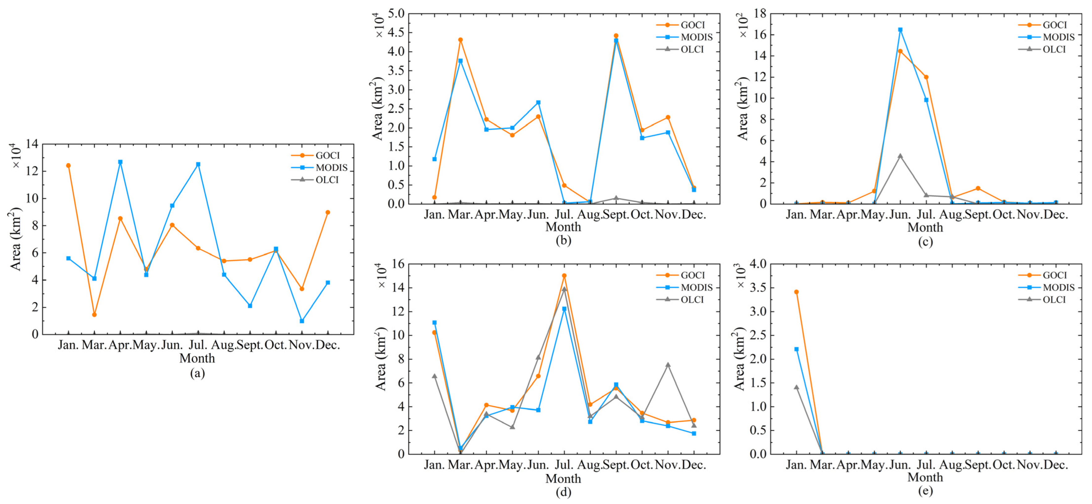
4.1. Spatial and Temporal Distribution of Marine Coverage Objects Contained in Data-Free Areas

The month-to-month variations of ocean objects in the data-free areas of each sensor have interesting trends (Figure 13). The missing amount of clean water is positively related to the missing amount of clouds, whereas the missing amount of turbid water has a significant inverse relationship. The missing amount of ocean coverage objects other than clouds in the data-free area of OLCI is much smaller than those of GOCI and MODIS. The number of missing elements does not vary much per month and tends to be stable. This phenomenon can be explained by the spatial and temporal distribution characteristics of typical marine coverage objects.
A typical altocumulus translucidus (Figure 14) is also known as a fish-scale cloud. It is a large-range regular cloud with large gaps between clouds, and the clouds have a fish scale-like arrangement [64]. As light can pass through the gaps, optical remote sensing also collects the remote sensing information of the sea surface corresponding to this gap. Such information is missing in GOCI and MODIS at this location (Figure 14b,e, respectively). The reason is that, depending on the ability of the selected cloud detection method, the normal ocean color information may be removed as a mask for cloud pixels [2,42]. A large amount of clean water information is lost. The normal ocean color information loss phenomenon occurs not only in the gaps between clouds but also at the edges of clouds. The irregular state appears as a missing internal fragment shape and a missing shape of edge patches. Usually, the edges of clouds tend to lose more ocean color information of cloud-free image pixels compared with the gaps between fish-scale clouds. By contrast, OLCI only misses the blocky cloud regions, and no anomalous missing information is observed. The normal ocean color information around the area is preserved, and the data-free area of OLCI manifests a fish-scale shape at this location (Figure 14h).
High outbreaks of green tide algae occur every summer, particularly in June and July (Figure 10c). The Yellow Sea is one of the areas of such an outbreak, and the phenomenon mainly occurs in the northward direction of the shallow shoals of the northern Jiangsu Province and the northeastern direction of the Jiaodong Peninsula. However, an analysis of GOCI and MODIS indicates that information is missing for the areas with high algal bloom (Figure 15).
The performance status of green algae in the data-free areas is different for the three products (Figure 15). Initially, the green tide algae in the ocean appear as small patches that float sporadically. Then, under the action of surface currents and summer monsoons, they continue to drift and grow. Finally, they gather into “stripes” and large patches corresponding to a green tide disaster [65]. The green tide algae in the data-free areas of GOCI and MODIS not only have spatial distributions appearing as circular spots and strips but also a buffer-like shape with missing pixels around them (Figure 15b,e, respectively). Similar to the missing cloud-free pixels around clouds, a missing algae-free pixel is apparent around green tide algae. The data-free areas containing green tide algae have spatially larger circular spots or appear to be connected with thick-striped distributions. As opposed to the missing information in GOCI and MODIS, the missing information in OLCI is only in the central area of the green tide algae with a high algal concentration and high phytoplankton contribution, and the missing pixels are scattered (i.e., not aggregated). Thus, it shows a sporadic distribution in space (Figure 15h).
As a surprising result of the year-round products, GOCI has missing information for all areas in the Yangtze River Delta region, whereas MODIS has missing information only to a lesser extent. OLCI is missing only the nearshore portion (Figure 16), retaining the majority of the muddy water pixels.
The largest turbidity zone in China exists in the Yangtze River Delta. The average depth of this shallow coastal zone is only 5–10 m. The high contribution of suspended particles is the main reason for the formation of turbidity zones, particularly the transport of Yangtze River currents, on the one hand, and the accumulation and resuspension of sediments in the Yellow Sea and East Sea due to the regional circulation of water masses on the other hand [24]. A large number of suspended particles accumulate in abundance to form the largest turbidity zone in China. However, suspended particles in the red and near-infrared wavelengths have a higher reflectivity than clean water, and they manifest near-cloud characteristics. These scenarios increase the difficulty of cloud detection and cause large losses among the products.
Except for the Yangtze River Delta region, the three kinds of data have frequent missing information for Liaodong Bay, Bohai Bay and Laizhou Bay (Figure 17a,d). GOCI has missing turbid and clean water information in these areas. MODIS is dominated by turbid water with less missing information compared with GOCI. The missing information in OLCI is negligible for the aforementioned three bay waters, and the quality of the product in this region is much better than those of MODIS and GOCI. The reason for the difference is that, in 2019, the Bohai Sea did not meet the first-category seawater quality standards in the ocean area of 12,740 square kilometers, accounting for about one-seventh of the entire Bohai Sea. The heavy eutrophic sea area was mainly concentrated in the denser population and more complex marine ecological environment of the three bays. The high planktonic biomass and heavy eutrophication conditions caused by anthropogenic nutrient inputs and fishing activities in coastal waters [66] can serve as the main reasons for the lack of product information in the waters of those areas.
The Bohai Sea is the highest latitude sea area in China. Owing to its special geographical location and the presence of cold air, the area suffers from different degrees of sea ice disasters in winter. The main geographic location of disasters is Liaodong Bay, and the ice period of sea ice is one to three months (December to February), which is annual sea ice [67]. The physicochemical properties of sea ice differ from those of clean water, but it is similar to clouds in remote sensing images with respect to color, temperature and highly reflective spectral properties [68,69]. Therefore, the product corresponding to the location of the sea ice hazard also suffers from missing information, i.e., the products suffer from missing information at that specific geographical location during the annual ice season. The identification of sea ice is much more difficult because of the similarity between sea ice and clouds in various aspects, and the identification effect is usually unsatisfactory. Thus, in this study, we opted to initially crop sea ice and some surrounding areas prior to analyzing them separately. Then, overall statistics and analyses were employed.
The data-free areas of GOCI and MODIS show sea ice similar to the shape of clouds, resulting in missing information and clumps aggregated without dispersion. These areas are located in the sea of Liaodong Bay, where the near-shore ecological environment is complex and where people usually gather. The pixels at the sea ice edge mainly correspond to turbid waters (eutrophic and high phytoplankton biology; Figure 18c,f). The thin ice areas of sea ice in OLCI generally do not cause missing information, but most thick ice areas are missing. As a result, the missing pixels have a fragmented distribution.
As opposed to the products of OLCI, the products of GOCI and MODIS do not usually appear separately for the different types of ocean coverage objects in the data-free area. For example, as shown in Figure 14, Figure 15, Figure 16 and Figure 17, clouds, green tide algae or turbid waters are usually accompanied by abundant clean water. Similarly, as shown in Figure 18, sea ice is surrounded by turbid water because this sea ice is located in Liaodong Bay, a region of the Bohai Sea that is heavily eutrophic all year round. The phenomenon of accompanying ocean cover objects in the data-free area is obvious. It can explain to a certain extent the over-representation of clean water in the data-free area.
The above discussion can also tentatively explain the phenomenon depicted in Figure 10. The missing amount of clean water in the data-free areas of GOCI and MODIS has a positive relationship with the missing amount of clouds, whereas the missing amount of turbid water has a significant inverse relationship. On the one hand, clean water, as a normal image element, should not appear to be masked. However, the concomitant effects of ocean cover objects in the data-free area and the concomitant occurrence of clouds and clean water bodies cause a phenomenon of increasing and decreasing. On the other hand, the information of turbid water pertaining to anomalous image pixels with high reflectivity may be masked as clouds [2]. However, clouds float over the ocean, and ocean color satellites can hardly penetrate clouds and fog. Clouds are given priority over turbid seawater during identification classification. Therefore, when clouds are in the same spatial position as seawater, they are identified as clouds. Clouds obscure turbid seawater when they are excessively large, thus causing a decrease in the sufficient identification of turbid water and vice versa. As a result, the missing amount of turbid water shows a significant inverse increase and decrease with the missing amount of clouds.

4.2. Analyses of the GOCI, MODIS and OLCI Ocean Color Product Differences

4.2.1. Cloud Detection Algorithm Variance Analysis

Figure 9, Figure 10, Figure 11, Figure 12 and Figure 13 show that GOCI and MODIS have striking similarities with respect to total missing rate, abnormal missing rate and the distribution of marine coverage objects. The number is much larger compared to OLCI.
To further explain the obtained result, we correlated the differences in cloud detection algorithms for the data. In the processing of ocean water color remote sensing, cloud masking usually considers the threshold method of Rayleigh scattering corrected reflectance ( ρ r c ) in the near-infrared band. The atmospheric correction scheme of using the Level 1 data of GOCI to generate the corresponding Level 2 data is the standard KOSC algorithm [70]. The algorithm is based on the SeaWiFS algorithm [71], and the threshold of ρ r c (865 nm) ≥ 0.028 is used to automatically mask cloud pixels in the standard atmospheric correction of the sensor. Moreover, the atmospheric correction scheme used by MODIS is the OCSSW algorithm in the NASA Earth Observation System SeaDAS software (i.e., it can automatically mask cloud pixels during atmospheric correction), with a threshold method of ρ r c (869 nm) ≥ 0.027 [2].
However, the methods only perform sufficiently at spatial locations in the open ocean, as some normal pixels are treated as masked clouds under complex ocean conditions. For example, high-sediment turbidity waters are prone to green tide algal hazards in summer, etc. [72]. The difference is that the atmospheric correction scheme used in OLCI is the Sen2Cor algorithm in the SNAP software, which simultaneously identifies and classifies clouds, cirrus, snow and water in the atmospheric correction step. The cloud mask effect in OLCI is much better than those in GOCI and MODIS, suggesting that the obtained ocean color products are also better with respect to information completeness and continuity quality. In contrast to GOCI and MODIS, the difference in the cloud detection selection bands is only 4 nm. It can be negligible and can be regarded as the same band signal, and the difference in the judgment thresholds is only 0.001. This contrast can help to explain the extremely high similarity between the spatial and temporal distribution characteristics of the data-free areas in GOCI and MODIS. Consequently, we selected the data-free area near the green tide algae mentioned above (Figure 15) and the surrounding pixels with retained information as the study area. Then, the different statuses of the spectral information within and around the data-free area were further explored. On the basis of the identification classification results, 80 sample points were evenly selected at the spatial location of green tide algae in the data-free area, the clean water location and the clean water location of the surrounding product data with retained information. A concomitant phenomenon of green tide algae is missing in the OLCI product. The green tide algae in the data-free areas are not adjacent to clean water. We selected the pixel of the retained reflectance of green tide algae in OLCI that is immediately adjacent to the data-free areas as the clean water in the data-free areas and then compared this with those in GOCI and MODIS. The reflectance values at the near-infrared band (GOCI: 865 nm, MODIS: 869.5 nm and OLCI: 865.3 nm) at the sample-point location of Level 1 data were obtained and then plotted as a box line graph.
As shown in Figure 19, the reflectance identified as pixels of the green tide algae in the data-free areas of the three data is generally high and fluctuating. The mean reflectance values at the spatial location of the green tide algae in all the data are near 0.045, 0.03 and 0.085. They are greater than the cloud mask threshold mentioned above. However, interestingly, the reflectance values of GOCI and MODIS in the clean water adjacent to the green tide algae within the data-free area do not fluctuate much, with both at less than 0.01, which is much smaller than the threshold of the cloud mask. The excellent cloud detection algorithm of OLCI allows the retention of valid ocean color information, even at spatial locations below 0.05 reflectance (Figure 19c). Furthermore, the range of the magnitudes of reflectance of clean water accompanying the green tide algae within the data-free areas of GOCI and MODIS is essentially the same as that of clean water with no missing information.
The cloud mask causes similar spatial and temporal distribution characteristics in the data-free areas of GOCI and MODIS when the environmental conditions within the ocean region are essentially the same. Thus, studying the accompanying phenomena of marine objects in the data-free area can provide a scientific basis for improving and optimizing cloud masks.

4.2.2. Spatial Resolution Difference Analysis

Different spatial resolutions affect the accuracy of classification results [73]. However, with respect to obtaining classification accuracy, a higher resolution scale (300–1000 m) implies a certain classification advantage. The spectral resolution and spectral range of MODIS are both greater than that of GOCI, but the classification accuracy of GOCI is greater than that of MODIS. Most of the MODIS bands are distributed in the range of 0.4–1 μm, and only three bands are in the range of 1–2.5 μm. Therefore, spatial resolution is more important than spectral resolution in obtaining high-classification accuracy at this scale.
On the one hand, the loss of fine patches caused by image pixel scale reduction is the main reason for accuracy reduction [74]. On the other hand, the spectral variability among the ocean objects of interest is large, and the spectral curves between them are discriminatory, as depicted by the target type that is clearly distinguishable from a small number of bands. As the spatial resolution of the image pixels becomes higher, the spectral consistency of the target image pixels becomes stronger, and improving the target classification accuracy becomes more beneficial. Therefore, increasing the spatial resolution is better than increasing the spectral resolution when identifying and classifying marine objects on this spatial scale. The overall accuracy of MODIS is the lowest at 89.3%, which is lower than the 91.9% of GOCI and 95.7% of OLCI. This finding indicates that 10.7% of the pixels in the data-free area of MODIS are misidentified, resulting in a systematic error in the statistics. This order also reflects their increasing spatial resolution from MODIS, GOCI and to OLCI. This undoubtedly reflects the importance of spatial resolution for obtaining excellent classification results at this spatial scale.
The accompanying phenomenon of the data-free area has been explained in this section with respect to the spatial resolution of data. The spatial resolution of ocean color satellites is generally low because of the vast area of the ocean and the large scale of the obtained data. Low spatial resolution data inevitably have mixed pixels. For example, in the case of the fish-scale clouds mentioned above, the low-resolution data have mixed pixels of clouds and clean water when gaps between the clouds are small. This scenario further affects the ability of the cloud detection algorithm and results in missing inter-cloud pixels. As shown in Figure 14c,f, the number of cloud pixel identification results of MODIS are more than those of GOCI because of the presence of mixed pixels. This is also the case in the turbid water of Figure 17. This difference can further explain the presence of concomitant phenomena in ocean-covered objects in data-free areas.

5. Conclusions

The ocean color products of the ocean cannot obtain effective results in special environments. For example, the concentrations of algal blooms are high in June and July each year in the shallow seas of northern Jiangsu to the Jiaodong Peninsula, the concentrations of suspended particles are high in the Yangtze River Delta, the anthropogenic activities are frequent, eutrophication differs among the three bays of the Bohai Sea, etc. Therefore, this study uses the proposed method to analyze and evaluate the data product information of the sea areas. We found that the missing data information is mostly due to the intensity difference of the cloud mask algorithm, which mistakenly identifies some marine coverage as clouds. On the one hand, certain temporal and spatial patterns are apparent in the data-free areas of the aforementioned products, obtaining a regular representation of common ocean-covered objects in time and space. On the other hand, a concomitant phenomenon between GOCI and MODIS has been determined for ocean coverage objects in data-free areas. Presumably, a concomitant phenomenon exists between the cloud mask algorithm results for the identification of marine targets of GOCI and MODIS. Therefore, the different product data should be optimized with respect to atmospheric correction and cloud detection to ensure the integrity and continuity of information. In particular, the missing information is the most serious GOCI and MODIS data.
In this study, the proposed ISAM algorithm was employed for the 2019 products of three ocean color satellites (i.e., GOCI, MODIS and OLCI). We obtained some characteristics of the data-free areas through detection. Then, we utilized the proposed ocean color information integrity and continuity indicators and applied them to three product evaluations while analyzing the spatial and temporal distribution characteristics of marine coverage objects in the data-free areas. The conclusions can be summarized as follows.
(1)
The integrity of the ocean colored product information is fundamentally based on the capability of the cloud detection algorithm. Most of the commonly used algorithms for cloud detection are the spectrum-oriented single-band or multi-band threshold methods. In this study, we employed an improved version of the spectrum-related SAM recognition algorithm and named it ISAM. The ISAM algorithm can reduce the fragmentation performance of the results and can increase the spatial continuity of the information. The ISAM algorithm can also reduce the fragmentation of the results, and it performs sufficiently in the recognition of marine objects. The obtained classification accuracy and Kappa coefficients are high. The ISAM algorithm is also applicable for multispectral data to a certain extent.
(2)
The spatial distributions of green tide algae and sea ice in the data-free areas of GOCI and MODIS are mainly manifested by the accompanying occurrence of their endmembers and the surrounding clean water. Sea ice is mostly accompanied by turbid water because of its geographical location. The shape performance of different ocean coverage objects varies, but a certain pattern can be observed over time. The number of green tide algae is higher in June and July every year, sea ice is most apparent from December to February and the missing amount in turbid waters is greater in spring and autumn. The absence of clean water shows a positive variation over time with cloud amount, mostly with the irregular spatial distribution around the accompanying clouds (above, below, left and right areas). By contrast, the missing amount of turbid water has an inverse variation over time with the cloud amount. The anomalous missing information in the data-free area of OLCI usually appears spatially as individual pixels or sporadic distribution of multiple pixels. The occurrence of accompanying phenomena is also rare, hence the minimal total amount of missing product information.
(3)
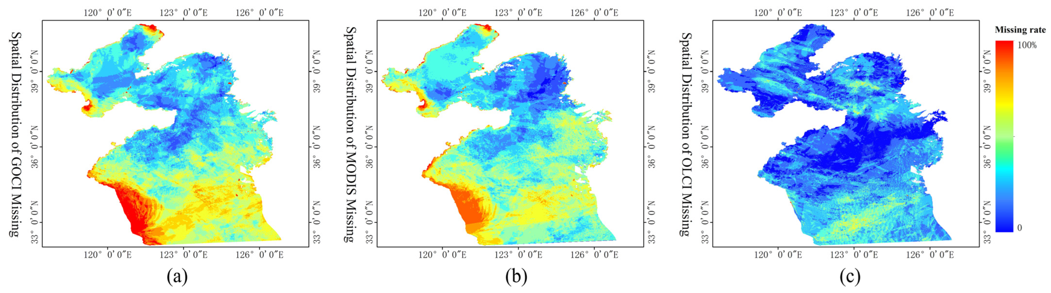
The experimental results (Table 5) indicate that the annual average missing rates of GOCI and MODIS are 25.81% and 27.04, respectively, which are much larger than the 10.05% of OLCI. In view of overcoming the effect of the perennial presence of clouds over the ocean, the anomalous missing rate is further used to measure the quality of product integrity. The experimental results show that the anomalous missing rates of GOCI and MODIS are 61.032% and 63.312%, respectively, which are much larger than the 1.115% of OLCI, and their anomalous missing rates are serious and similar, in general. The quality of the three products was evaluated from the perspective of integrity. The results indicate that OLCI is the superior product, followed by GOCI. Among the three products, MODIS has the worst integrity quality.
(4)
During the research process, we found that the data-free area has certain spatial and temporal distribution characteristics. Subsequently, we calculated the results of the spatiotemporal images of the data-free area to evaluate the product quality with respect to temporal and spatial patterns. Standard deviation and information entropy were applied to the spatiotemporal images for the quantitative evaluation of the information continuity of the ocean color products. The results (Table 7) indicate that OLCI is superior to GOCI and MODIS with respect to the spatiotemporal continuity of product information. However, as opposed to the results of the data information integrity evaluation, MODIS is superior to GOCI with respect to spatiotemporal continuity of information. In summary, OLCI is optimal with respect to both information integrity and the continuity of information.
The ISAM algorithm can automatically determine the optimal threshold value for classification, thus improving the spatial continuity and accuracy of the results. The proposed method is a new reliable technical method that can support the recognition of target objects at sea. The data selected in this study are based on a unit of the four seasons, with three images per season (two images in winter) and a total of 33 scenes from three kinds of satellite data. Given the limitations in the statistical results, multi-scene images can be selected with a unit of months in future research. In principle, our method can be applied to other ocean color satellite data (e.g., GOCI-II, SwaWiFS, etc.), but further work is needed. The obtained results for the Yellow and Bohai seas can be applied to other coastal regions in the World Ocean. The new method can objectively and subjectively analyze and evaluate the information in the product data-free area. Overall, this study can enrich the evaluation of ocean color products, and it provides a new direction for the optimization of atmospheric correction and cloud detection methods for ocean color data. Using different time series and different satellite combination data to fill data-free areas may be the future direction. It provides a certain reference value for producers and users in the aspect of product selection.

Author Contributions

Conceptualization, S.Z. and H.Z.; methodology, S.Z. and H.Z.; validation, S.Z., H.Z. and H.L.; formal analysis, S.Z. and H.Z.; investigation, S.Z. and H.Z.; writing—original draft preparation, S.Z.; writing—review and editing, S.Z., H.Z., J.L. and Y.Y.; visualization, S.Z.; supervision, H.Z.; funding acquisition, H.Z. and H.L. All authors have read and agreed to the published version of the manuscript.

Funding

This research was funded by the auspices of the National Natural Science Foundation of China (Grant No. 41971339), the National Key Research and Development Project of China (No. 2018YFC1407605) and the SDUST Research Fund (No. 2019TDJH103).

Data Availability Statement

Not applicable.

Acknowledgments

We thank the following institutions for their kind assistance with this research: the National Marine Environmental Monitoring Center for providing the actual measurement data to serve as a guide; the Korea Ocean Satellite Center for providing the GOCI data; the National Aeronautics and Space Administration for providing the MODIS data; and the European Organisation for the Exploitation of Meteorological Satellites for providing the OLCI data.

Conflicts of Interest

The authors declare no conflict of interest.

References

  1. Cui, T.; Zhang, J.; Tang, J.; Sathyendranath, S.; Groom, S.; Ma, Y.; Zhao, W.; Song, Q. Assessment of satellite ocean color products of MERIS, MODIS and SeaWiFS along the East China Coast (in the Yellow Sea and East China Sea). ISPRS J. Photogramm. Remote Sens. 2014, 87, 137–151. [Google Scholar] [CrossRef]
  2. Lu, S.; He, M.; He, S.; He, S.; Pan, Y.; Yin, W.; Li, P. An Improved Cloud Masking Method for GOCI Data over Turbid Coastal Waters. Remote Sens. 2021, 13, 2722. [Google Scholar] [CrossRef]
  3. Borge, O.M.; Bakken, S.; Johansen, T.A. Atmospheric Correction of Hyperspectral Data Over Coastal Waters Based on Machine Learning Models. In Proceedings of the 2021 11th Workshop on Hyperspectral Imaging and Signal Processing: Evolution in Remote Sensing (WHISPERS), Amsterdam, The Netherlands, 24–26 March 2021; pp. 1–5. [Google Scholar] [CrossRef]
  4. Gilerson, A.; Malinowski, M.; Herrera, E.; Tomlinson, M.C.; Stumpf, R.P.; Ondrusek, M.E. Estimation of chlorophyll-a concentration in complex coastal waters from satellite imagery. In Proceedings of the Conference on Ocean Sensing and Monitoring XIII, Electr Network, Online, 12–16 April 2021; Volume 11752. [Google Scholar]
  5. Ji, T.-Y.U.; Yokoya, N.; Zhu, X.X.; Huang, T.-Z. Nonlocal Tensor Completion for Multitemporal Remotely Sensed Images’ Inpainting. IEEE Trans. Geosci. Remote Sens. 2018, 56, 3047–3061. [Google Scholar] [CrossRef]
  6. Shen, H.; Li, X.; Cheng, Q.; Zeng, C.; Yang, G.; Li, H.; Zhang, L. Missing Information Reconstruction of Remote Sensing Data: A Technical Review. IEEE Geosci. Remote Sens. Mag. 2015, 3, 61–85. [Google Scholar] [CrossRef]
  7. Choi, Y.-H.; Lee, W.-J.; Park, S.-C.; Sun, J.; Lee, D.K. Retrieving Volcanic Ash Information Using COMS Satellite (MI) and Landsat-8 (OLI, TIRS) Satellite Imagery: A Case Study of Sakurajima Volcano. Korean J. Remote Sens. 2017, 33, 587–598. [Google Scholar]
  8. Hooker, S.B.; Mcclain, C.R. The calibration and validation of SeaWiFS data. Prog. Oceanogr. 2000, 45, 427–465. [Google Scholar] [CrossRef] [Green Version]
  9. Białek, A.; Vellucci, V.; Gentil, B.; Antoine, D.; Gorroño, J.; Fox, N.; Underwood, C. Monte Carlo–Based Quantification of Uncertainties in Determining Ocean Remote Sensing Reflectance from Underwater Fixed-Depth Radiometry Measurements. J. Atmos. Ocean. Technol. 2020, 37, 177–196. [Google Scholar] [CrossRef]
  10. Joshi, I.D.; D’Sa, E.J. Optical Properties Using Adaptive Selection of NIR/SWIR Reflectance Correction and Quasi-Analytic Algorithms for the MODIS-Aqua in Estuarine-Ocean Continuum: Application to the Northern Gulf of Mexico. IEEE Trans. Geosci. Remote Sens. 2020, 58, 6088–6105. [Google Scholar] [CrossRef]
  11. Al-Naimi, N.; Raitsos, D.E.; Ben-Hamadou, R.; Soliman, Y. Evaluation of Satellite Retrievals of Chlorophyll-a in the Arabian Gulf. Remote Sens. 2017, 9, 301. [Google Scholar] [CrossRef] [Green Version]
  12. Jiang, L.L.; Guo, X.; Wang, L.; Sathyendranath, S.; Evers-King, H.; Chen, Y.; Li, B. Validation of MODIS ocean-colour products in the coastal waters of the Yellow Sea and East China Sea. Acta Oceanol. Sin. 2020, 39, 91–101. [Google Scholar] [CrossRef]
  13. Rodríguez-Esparragón, D.; Marcello, J.; Eugenio, F.; García-Pedrero, A.; Gonzalo-Martín, C. Object-based quality evaluation procedure for fused remote sensing imagery. Neurocomputing 2017, 255, 40–51. [Google Scholar] [CrossRef]
  14. Wang, N.N.; Gao, X.B.; Tao, D.C.; Yang, H.; Li, X.L. Facial feature point detection: A comprehensive survey. Neurocomputing 2018, 275, 50–65. [Google Scholar] [CrossRef] [Green Version]
  15. Zhou, W.; Bovik, A.C. Modern Image Quality Assessment. Synth. Lect. Image Video Multimed. Process. 2006, 2, 156. [Google Scholar] [CrossRef] [Green Version]
  16. Bosse, S.; Maniry, D.; Müller, K.; Wiegand, T.; Samek, W. Deep Neural Networks for No-Reference and Full-Reference Image Quality Assessment. IEEE Trans. Image Process. 2018, 27, 206–219. [Google Scholar] [CrossRef] [Green Version]
  17. Sheikh, H.R.; Bovik, A.C. Image information and visual quality. IEEE Trans Image Process. 2006, 15, 430–444. [Google Scholar] [CrossRef] [PubMed]
  18. Shannon, C.E. A Mathematical Theory of Communication. Bell Syst. Tech. J. 1948, 27, 623–656. [Google Scholar] [CrossRef]
  19. Shannon, C.E. The mathematical theory of communication. Bell Labs Tech. J. 1950, 3, 31–32. [Google Scholar] [CrossRef] [Green Version]
  20. Zhu, P.; Jiang, Z.; Zhang, J.L.; Zhang, Y.; Wu, P. Remote sensing image watermarking based on motion blur degeneration and restoration model. Optik 2021, 248, 168018. [Google Scholar] [CrossRef]
  21. Okarma, K. Current Trends and Advances in Image Quality Assessment. Elektron. Ir Elektrotechnika 2019, 25, 77–84. [Google Scholar] [CrossRef] [Green Version]
  22. Balanov, A.; Schwartz, A.; Moshe, Y. Reduced-reference image quality assessment based on DCT Subband Similarity. In Proceedings of the 2016 Eighth International Conference on Quality of Multimedia Experience (QoMEX), Lisbon, Portugal, 6–8 June 2016; pp. 1–6. [Google Scholar] [CrossRef]
  23. Wu, J.J.; Lin, W.S.; Shi, G.M.; Liu, A.M. Reduced-Reference Image Quality Assessment With Visual Information Fidelity. IEEE Trans. Multimed. 2013, 15, 1700–1705. [Google Scholar] [CrossRef]
  24. Park, J.-E.; Park, K.-A.; Lee, J.-H. Overview and Prospective of Satellite Chlorophyll-a Concentration Retrieval Algorithms Suitable for Coastal Turbid Sea Waters. J. Korean Earth Sci. Soc. 2021, 42, 247–263. [Google Scholar] [CrossRef]
  25. Hu, Z.; Pan, D.; He, X.; Song, D.; Huang, N.; Bai, Y.; Xu, Y.; Wang, X.; Zhang, L.; Gong, F. Assessment of the MCC method to estimate sea surface currents in highly turbid coastal waters from GOCI. Int. J. Remote Sens. 2017, 38, 572–597. [Google Scholar] [CrossRef]
  26. Pan, Y.; Shen, F.; Verhoef, W. An improved spectral optimization algorithm for atmospheric correction over turbid coastal waters: A case study from the Changjiang (Yangtze) estuary and the adjacent coast. Remote Sens. Environ. 2017, 191, 197–214. [Google Scholar] [CrossRef] [Green Version]
  27. Shen, F.; Salama, M.H.D.S.; Zhou, Y.-X.; Li, J.-F.; Su, Z.; Kuang, D.-B. Remote-sensing reflectance characteristics of highly turbid estuarine waters—A comparative experiment of the Yangtze River and the Yellow River. Int. J. Remote Sens. 2010, 31, 2639–2654. [Google Scholar] [CrossRef]
  28. Zibordi, G.; Melin, F.; Berthon, J.-F. A Regional Assessment of OLCI Data Products. IEEE Geosci. Remote Sens. Lett. 2018, 15, 1490–1494. [Google Scholar] [CrossRef]
  29. Wojtasiewicz, B.; Hardman-Mountford, N.J.; Antoine, D.; Dufois, F.; Slawinski, D.; Trull, T.W. Use of bio-optical profiling float data in validation of ocean colour satellite products in a remote ocean region. Remote Sens. Environ. 2018, 209, 275–290. [Google Scholar] [CrossRef]
  30. Li, H.; He, X.; Ding, J.; Hu, Z. Validation of the Remote Sensing Products Retrieved by Geostationary Ocean Color Imager in Liaodong Bay in Spring. Acta Opt. Sin. 2016, 36, 17–28. [Google Scholar] [CrossRef]
  31. Melin, F. From Validation Statistics to Uncertainty Estimates: Application to VIIRS Ocean Color Radiometric Products at European Coastal Locations. Front. Mar. Sci. 2021, 8, 790948. [Google Scholar] [CrossRef]
  32. Fu, L.Z.; Qu, Y.H.; Wang, J.D. Bias analysis in validation of modis lai product: A case study in cropland of Huailai, northern China. In Proceedings of the 36th IEEE International Geoscience and Remote Sensing Symposium (IGARSS), Beijing, China, 10–15 July 2016; pp. 5921–5924. [Google Scholar] [CrossRef]
  33. Guo, J.; Liu, X.; Xie, Q. Characteristics of the Bohai Sea oil spill and its impact on the Bohai Sea ecosystem. Chin. Sci. Bull. 2012, 58, 2276–2281. [Google Scholar] [CrossRef] [Green Version]
  34. Ryu, J.-H.; Han, H.-J.; Cho, S.; Park, Y.-J.; Ahn, Y.-H. Overview of geostationary ocean color imager (GOCI) and GOCI data processing system (GDPS). Ocean Sci. J. 2012, 47, 223–233. [Google Scholar] [CrossRef]
  35. Choi, J.-K.; Park, Y.J.; Ahn, J.H.; Lim, H.-S.; Eom, J.; Ryu, J.-H. GOCI, the world’s first geostationary ocean color observation satellite, for the monitoring of temporal variability in coastal water turbidity. J. Geophys. Res. Ocean. 2012, 117, 9004. [Google Scholar] [CrossRef]
  36. Song, Q.J.; Chen, S.; Xue, C.; Lin, M.; Du, K.; Li, S.; Ma, C.; Tang, J.; Liu, J.; Zhang, T.; et al. Vicarious calibration of COCTS-HY1C at visible and near-infrared bands for ocean color application. Opt. Express 2019, 27, A1615–A1626. [Google Scholar] [CrossRef]
  37. Wang, M.; Shi, W. Sensor Noise Effects of the SWIR Bands on MODIS-Derived Ocean Color Products. IEEE Trans. Geosci. Remote Sens. 2012, 50, 3280–3292. [Google Scholar] [CrossRef]
  38. Kappas, M.; Phan, T.N. Application of MODIS land surface temperature data: A systematic literature review and analysis. J. Appl. Remote Sens. 2018, 12, 1. [Google Scholar] [CrossRef]
  39. Hammond, M.L.; Henson, S.A.; Lamquin, N.; Clerc, S.; Donlon, C. Assessing the Effect of Tandem Phase Sentinel-3 OLCI Sensor Uncertainty on the Estimation of Potential Ocean Chlorophyll-a Trends. Remote Sens. 2020, 12, 2522. [Google Scholar] [CrossRef]
  40. Tilstone, G.H.; Pardo, S.; Dall’Olmo, G.; Brewin, R.J.W.; Nencioli, F.; Dessailly, D.; Kwiatkowska, E.; Casal, T.; Donlon, C. Performance of Ocean Colour Chlorophyll a algorithms for Sentinel-3 OLCI, MODIS-Aqua and Suomi-VIIRS in open-ocean waters of the Atlantic. Remote Sens. Environ. 2021, 260, 112444. [Google Scholar] [CrossRef]
  41. Zibordi, G.; Talone, M.; Voss, K.J.; Johnson, B.C. Impact of spectral resolution of in situ ocean color radiometric data in satellite matchups analyses. Opt Express 2017, 25, A798–A812. [Google Scholar] [CrossRef] [Green Version]
  42. Chen, S.; Zhang, T. An improved cloud masking algorithm for MODIS ocean colour data processing. Remote Sens. Lett. 2015, 6, 218–227. [Google Scholar] [CrossRef]
  43. Meng, Q.; Mao, Z.; Huang, H.; Shen, Y. Inversion of suspended sediment concentration at the Hangzhou Bay based on the high-resolution satellite HJ-1A/B imagery. Proc. SPIE Int. Soc. Opt. Eng. 2013, 8869, 8. [Google Scholar] [CrossRef]
  44. Jiang, B.; Li, H.; Teng, G.; Yan, J.; Zhang, B. Using GOCI extracting information of red tide for time-series analysing in East China Sea. J. Zhejiang Univ. 2017, 44, 576–583. [Google Scholar] [CrossRef]
  45. Boardman, J.W.; Kruse, F.A.; Green, R.O. Mapping Target Signatures via Partial Unmixing of AVIRIS Data; JPL Publication: Pasadena, CA, USA, 1995; pp. 23–26. [Google Scholar]
  46. Du, B.; Wei, Q.; Liu, R. An Improved Quantum-Behaved Particle Swarm Optimization for Endmember Extraction. IEEE Trans. Geosci. Remote Sens. 2019, 57, 6003–6017. [Google Scholar] [CrossRef]
  47. Cui, T.-W.; Zhang, J.; Sun, L.-E.; Jia, Y.-J.; Zhao, W.; Wang, Z.-L.; Meng, J.-M. Satellite monitoring of massive green macroalgae bloom (GMB): Imaging ability comparison of multi-source data and drifting velocity estimation. Int. J. Remote Sens. 2012, 33, 5513–5527. [Google Scholar] [CrossRef]
  48. Yuan, C.; Zhang, J.; Xiao, J.; Fu, M.; Zhang, X.; Cui, T.; Wang, Z. The spatial and temporal distribution of floating green algae in the Subei Shoal in 2018 retrieved by Sentinel-2 images. Haiyang Xuebao 2020, 42, 12–20. [Google Scholar] [CrossRef]
  49. Kruse, F.A.; Lefkoff, A.B.; Boardman, J.W.; Heidebrecht, K.B.; Shapiro, A.T.; Barloon, P.J.; Goetz, A.F.H. The spectral image processing system (SIPS)—interactive visualization and analysis of imaging spectrometer data. Remote Sens. Environ. 1993, 44, 145–163. [Google Scholar] [CrossRef]
  50. Lin, C.-H.; Tsai, P.-H.; Lai, K.-H.; Chen, J.-Y. Cloud Removal From Multitemporal Satellite Images Using Information Cloning. IEEE Trans. Geosci. Remote Sens. 2013, 51, 232–241. [Google Scholar] [CrossRef]
  51. Sohn, Y.; Rebello, N.S. Supervised and unsupervised spectral angle classifiers. Photogramm. Eng. Remote Sens. 2002, 68, 1271–1280. [Google Scholar] [CrossRef]
  52. Furukawa, F.; Morimoto, J.; Yoshimura, N.; Kaneko, M. Comparison of Conventional Change Detection Methodologies Using High-Resolution Imagery to Find Forest Damage Caused by Typhoons. Remote Sens. 2020, 12, 3242. [Google Scholar] [CrossRef]
  53. Baker, C.; Lawrence, R.; Montagne, C.; Patten, D.J.W. Mapping Wetlands and Riparian Areas Using Landsat ETM+ Imagery and Decision-Tree-Based Models. Wetlands 2006, 26, 465–474. [Google Scholar] [CrossRef]
  54. Liu, Y.; Lu, S.; Lu, X.; Wang, Z.; Chen, C.; He, H. Classification of Urban Hyperspectral Remote Sensing Imagery Based on Optimized Spectral Angle Mapping. J. Indian Soc. Remote Sens. 2019, 47, 289–294. [Google Scholar] [CrossRef]
  55. Li, M.; Zhang, P. Classification of Wetland Vegetation in Hyperspectral Remote Sensing Image Based on SAM Algorithm. For. Eng. 2015, 31, 8–13. [Google Scholar] [CrossRef]
  56. Tian, L.; Sun, X.; Li, J.; Xing, Q.; Song, Q.; Tong, R. Sampling Uncertainties of Long-Term Remote-Sensing Suspended Sediments Monitoring over China’s Seas: Impacts of Cloud Coverage and Sediment Variations. Remote Sens. 2020, 12, 1945. [Google Scholar] [CrossRef]
  57. Coluzzi, R.; Imbrenda, V.; Lanfredi, M.; Simoniello, T. A first assessment of the Sentinel-2 Level 1-C cloud mask product to support informed surface analyses. Remote Sens. Environ. 2018, 217, 426–443. [Google Scholar] [CrossRef]
  58. Leinenkugel, P.; Kuenzer, C.; Dech, S. Comparison and enhancement of MODIS cloud mask products for Southeast Asia. Int. J. Remote Sens. 2013, 34, 2730–2748. [Google Scholar] [CrossRef]
  59. Chen, S.; Du, K.; Lee, Z.; Liu, J.; Song, Q.; Xue, C.; Wang, D.; Lin, M.; Tang, J.; Ma, C. Performance of COCTS in Global Ocean Color Remote Sensing. IEEE Trans. Geosci. Remote Sens. 2021, 59, 1634–1644. [Google Scholar] [CrossRef]
  60. Hu, C.; Le, C. Ocean Color Continuity From VIIRS Measurements Over Tampa Bay. IEEE Geosci. Remote Sens. Lett. 2014, 11, 945–949. [Google Scholar] [CrossRef]
  61. Liu, J.; Huang, J.; Liu, S.; Li, H.; Zhou, Q.; Liu, J. Human visual system consistent quality assessment for remote sensing image fusion. ISPRS J. Photogramm. Remote Sens. 2015, 105, 79–90. [Google Scholar] [CrossRef]
  62. Petty, G.W. On Some Shortcomings of Shannon Entropy as a Measure of Information Content in Indirect Measurements of Continuous Variables. J. Atmos. Ocean. Technol. 2018, 35, 1011–1021. [Google Scholar] [CrossRef]
  63. Liu, L.; Zhou, F.; Tao, M.; Sun, P.; Zhang, Z. Adaptive Translational Motion Compensation Method for ISAR Imaging Under Low SNR Based on Particle Swarm Optimization. IEEE J. Sel. Top. Appl. Earth Obs. Remote Sens. 2015, 8, 5146–5157. [Google Scholar] [CrossRef]
  64. Govender, P.; Sivakumar, V. Investigating diffuse irradiance variation under different cloud conditions in Durban, using k-means clustering. J. Energy South. Afr. 2019, 30, 22–32. [Google Scholar] [CrossRef]
  65. Wang, Z.; Xiao, J.; Fan, S.; Li, Y.; Liu, X.; Liu, D. Who made the world’s largest green tide in China?-an integrated study on the initiation and early development of the green tide in Yellow Sea. Limnol. Oceanogr. 2015, 60, 1105–1117. [Google Scholar] [CrossRef]
  66. Galloway, J.N.; Townsend, A.R.; Erisman, J.W.; Bekunda, M.; Cai, Z.; Freney, J.R.; Martinelli, L.A.; Seitzinger, S.P.; Sutton, M.A. Transformation of the nitrogen cycle: Recent trends, questions, and potential solutions. Science 2008, 320, 889–892. [Google Scholar] [CrossRef] [PubMed] [Green Version]
  67. Yan, Y.; Huang, K.; Shao, D.; Xu, Y.; Gu, W. Monitoring the Characteristics of the Bohai Sea Ice Using High-Resolution Geostationary Ocean Color Imager (GOCI) Data. Sustainability 2019, 11, 777. [Google Scholar] [CrossRef] [Green Version]
  68. Miao, X.; Xie, H.; Ackley, S.F.; Perovich, D.K.; Ke, C. Object-based detection of Arctic sea ice and melt ponds using high spatial resolution aerial photographs. Cold Reg. Sci. Technol. 2015, 119, 211–222. [Google Scholar] [CrossRef]
  69. Ouyang, L.; Hui, F.; Zhu, L.; Cheng, X.; Zeng, T. The spatiotemporal patterns of sea ice in the Bohai Sea during the winter seasons of 2000–2016. Int. J. Digit. Earth 2017, 12, 893–909. [Google Scholar] [CrossRef]
  70. Ahn, J.-H.; Park, Y.-J.; Ryu, J.-H.; Lee, B.; Oh, I.S. Development of atmospheric correction algorithm for Geostationary Ocean Color Imager (GOCI). Ocean Sci. J. 2012, 47, 247–259. [Google Scholar] [CrossRef]
  71. Gordon, H.R.; Wang, M.J.A.O. Retrieval of water-leaving radiance and aerosol optical thickness over the oceans with SeaWiFS: A preliminary algorithm. Appl. Opt. 1994, 33, 443–452. [Google Scholar] [CrossRef]
  72. Banks, A.C.; Mélin, F. An assessment of cloud masking schemes for satellite ocean colour data of marine optical extremes. Int. J. Remote Sens. 2015, 36, 797–821. [Google Scholar] [CrossRef] [Green Version]
  73. Nguyen-Van-Anh, V.; Hoang-Phi, P.; Nguyen-Kim, T.; Lam-Dao, N.; Vu, T.T. The influence of satellite image spatial resolution on mapping land use/land cover: A case study of Ho Chi Minh City, Vietnam. IOP Conf. Ser. Earth Environ. Sci. 2021, 652, 012002. [Google Scholar] [CrossRef]
  74. Wang, L.; Liu, J.; Gao, J.; Yang, L.; Yang, F.; Wang, X. Relationship between accuracy of winter wheat area remote sensing identification and spatial resolution. Trans. Chin. Soc. Agric. Eng. 2016, 32, 152–160. [Google Scholar] [CrossRef]
Figure 1. Location of the study area in the Yellow Sea and Bohai Sea.
Remotesensing 14 03815 g001
Figure 2. Framework and technical methods.
Remotesensing 14 03815 g002
Figure 3. Extraction results and spatial location determination of green tide algae: (a) GOCI, (b) MODIS and (c) OLCI.
Remotesensing 14 03815 g003
Figure 4. Schematic diagram of the cloud inspection workflow.
Remotesensing 14 03815 g004
Figure 5. Cloud detection results and spatial location determination: (a) GOCI, (b) MODIS and (c) OLCI.
Remotesensing 14 03815 g005
Figure 6. Spectral information of the endmembers of the ocean coverage object: (a) GOCI, (b) MODIS and (c) OLCI.
Remotesensing 14 03815 g006
Figure 7. Schematic diagram of the SAM recognition classification principle.
Remotesensing 14 03815 g007
Figure 8. Diagram of the processing result of the Clump method (Red for clouds, green for green tide, blue for clean water): (a) pre-method results and (b) post-method results.
Remotesensing 14 03815 g008
Figure 9. Diagram of month-by-month missing rate: (a) box line diagram and (b) line graph.
Remotesensing 14 03815 g009
Figure 10. Schematic diagram of the distribution of total missing marine coverage types for all seasons for the three products: (a) clean water, (b) turbid water, (c) green tide algae, (d) clouds and (e) sea ice.
Remotesensing 14 03815 g010
Figure 11. Schematic of the abnormal missing areas and proportions over four seasons (month by month): (a) area and (b) percentage.
Remotesensing 14 03815 g011
Figure 12. Schematic of the spatiotemporal image of the data-free area: (a) GOCI, (b) MODIS and (c) OLCI.
Remotesensing 14 03815 g012
Figure 13. Schematic diagram of the month-by-month change in marine objects in the data-free areas: (a) GOCI, (b) MODIS and (c) OLCI.
Remotesensing 14 03815 g013
Figure 14. Schematic diagram of the missing position of altocumulus translucidus: (a,d,g) the true color images at the spatial locations of the altocumulus translucidus for GOCI, MODIS and OLCI data, respectively; (b,e,h) the condition of the data-free area; (c,f,i) the identification status of the marine objects in the data-free area.
Remotesensing 14 03815 g014
Figure 15. Schematic diagram of green tide algae in the data-free areas: (a,d,g) the true color images at the spatial locations of the green tide algae for GOCI, MODIS and OLCI data, respectively; (b,e,h) the condition of the data-free area; (c,f,i) the identifi-cation status of the marine objects in the data-free area.
Remotesensing 14 03815 g015
Figure 16. Schematic diagram of the missing OLCI data in the Yangtze River Delta region (Red for clouds, yellow for turbid water).
Remotesensing 14 03815 g016
Figure 17. Schematic diagram of turbid water in the data-free areas: (a,d,g) the true color images at the spatial locations of the turbid water for GOCI, MODIS and OLCI data, respectively; (b,e,h) the condition of the data-free area; (c,f,i) the identifi-cation status of the marine objects in the data-free area. The red boxes in (a,d,g) represent the main turbid water areas.
Remotesensing 14 03815 g017
Figure 18. Schematic diagram of sea ice in the data-free areas: (a,d,g) the true color images at the spatial locations of the sea ice for GOCI, MODIS and OLCI data, respectively; (b,e,h) the condition of the data-free area; (c,f,i) the identifi-cation status of the marine objects in the data-free area.
Remotesensing 14 03815 g018
Figure 19. The reflectance of green tide algae, clean water in the data-free area and clean water in the area with retained information: (a) GOCI, (b) MODIS and (c) OLCI.
Remotesensing 14 03815 g019
Table 1. Parameters of the GOCI, MODIS and OLCI satellite sensors.
DataSatelliteBand NumberSpectrum
Range   ( μ m )
Spatial
Resolution (m)
Temporal
Resolution (Day)
GOCICOMS80.412–0.8655000.05
MODISTerra/Aqua36 (1,2/3–7/8–36)0.412–14.38250/500/10001
OLCISentinel 3210.4–1.02300<2
Table 2. Product introduction.
DataLevel 1Level 2
GOCICOMS_GOCI_L1BCOMS_GOCI_L2A
MODISMOD02KML2_LAC_OC
OLCIOL_1_EFROL_2_WFR
Table 3. Threshold values for each type of object.
Radians (R)GOCIMODISOLCI
Open Sea0.2350.3250.260
Turbid Water0.1750.2400.265
Green Tide0.3600.2950.320
Sea Ice0.1250.1550.110
Cloud0.5850.6300.525
Table 4. Threshold values for each type of object accuracy evaluation of classification results.
SensorsProducer Accuracy (%)User Accuracy (%)Kappa CoefficientOverall Accuracy (%)
GOCI84.894.60.9091.9
MODIS92.490.70.8689.3
OLCI80.491.40.8995.7
Table 5. Month-by-month missing rate of the three products.
Miss Rate (%)GOCIMODISOLCI
Jan.43.6339.2313.24
Mar.11.5018.230.11
Apr.28.0538.796.72
May.19.3822.424.56
Jun.32.1334.7916.20
Jul.41.3653.9927.66
Aug.18.1515.586.36
Sept.29.2026.619.87
Oct.21.8123.556.21
Nov.15.6411.3814.89
Dec.23.1012.904.75
AVG25.8127.0410.05
Table 6. Status of the proportion of marine coverage objects in the data-free areas.
ClassGOCIMODISOLCI
Area (km2)Percentage (%)Area (km2)Percentage (%)Area (km2)Percentage (%)
Open Sea709,86147.07777.135663,92648.42276.4811683.180.30227.044
Turbid Water203,98213.52822.165199,28414.53422.9562536.920.45540.762
Green Tide3030.250.2010.32926760.1950.308599.850.1089.638
Sea Ice34130.2260.37122100.1610.2551403.820.25222.556
Cloud587,599.7538.968 503,03836.688 551,769.0398.885
Abnormal Missing920,286.2561.032868,09663.3126223.771.115
Total1,507,8861001,371,134100557,992.8100
Table 7. Spatiotemporal continuity indicators.
FactorGOCIMODISOLCI
Standard
Deviation (%)
3.153.052.12
Information
Entropy (bit)
15.5113.9310.13
Publisher’s Note: MDPI stays neutral with regard to jurisdictional claims in published maps and institutional affiliations.

