1. Introduction
Small unmanned aerial vehicles (UAVs) equipped with imaging sensor systems such as ALADIN or MIKADO of the German Armed Forces operate at relatively low altitudes (ca. 30–150 m) and are commonly utilized for reconnaissance tasks in tactical environments, as they are quickly deployed and allow to monitor very large areas without directly risking human lives. However, military forces generally attempt to conceal themselves and their equipment in their respective environments by using camouflage, making tactical reconnaissance a particularly demanding challenge. Additionally, small tactical reconnaissance drones are usually equipped with rudimentary visual or thermal sensor systems, which do not necessarily provide enough information in order to distinguish between camouflaged objects and their surroundings. Deploying a sensor payload that provides spectral information beyond visual or thermal range could therefore be crucial for the detection of camouflaged objects, as camouflage might lose its effectiveness in certain spectral regions.
Hyperspectral imaging systems, for instance, are capable of capturing a unique and distinctive spectral signature of every physical material, which can be successfully exploited for camouflage detection [
1,
2]. However, considering a tactical environment with small reconnaissance drones, the size, weight, power, and cost criteria (SWaP-C) of any payload must be taken into account. As powerful as hyperspectral sensors can be, as expensive is their acquisition. In addition, raw hyperspectral sensor data requires extensive postprocessing in order to obtain a hyperspectral data cube, rendering online hyperspectral sensor data evaluation nearly impossible. Compared to hyperspectral sensor systems, multispectral sensor systems generally come at a more favorable price, are lower in size and weight and require much less postprocessing, making them considerably more relevant for any airborne remote sensing application. Yet, their spectral resolution is significantly lower and their spectral sensitivity per band is significantly higher, which could diminish their practical value in other ways.
Nevertheless, multispectral imagery has found many applications in recent years, ranging from precision farming [
3,
4,
5,
6], vegetational monitoring [
7,
8,
9,
10,
11,
12] and disturbance detection [
13,
14,
15] to biomass estimation [
16], aquatic plant detection [
17,
18], bathymetry [
19], and even camouflage detection [
20]. In [
20], constrained energy minimization (CEM) in combination with a customized version of the well-known OTSU thresholding algorithm is applied to detect multiple camouflages in complex outdoor scenes of different perspectives. In addition to the effectiveness of the proposed method, it requires prior spectral knowledge about the camouflage, which might not be available in real-world tactical reconnaissance scenarios.
Since multispectral imagery has already been proven for various applications, even camouflage detection, the Institute of Flight Systems of the Universität der Bundeswehr München is actively researching the possibilities of multispectral imaging systems in tactical reconnaissance scenarios for computer-aided near real-time camouflage detection. For this purpose, a multispectral sensor setup was composed, mounted on a commercial drone, and utilized to collect a multispectral dataset containing multiple camouflaged targets of different materials and sizes. Moreover, a set of four well-known methods for hyperspectral anomaly detection (RX [
21], LRX [
21], CRD [
22], and AED [
23]) and one new density-based method developed by the authors called local point density (LPD) were adopted and applied on the specially created multispectral dataset. In addition to the raw dataset, the methods were also applied on an extension with multiple vegetation indices (BNDVI, GNDVI, and NDRE) of it, as they appeared to have increased contrast between the targets and their surroundings. The performance of these methods for detecting the camouflaged targets in the data were evaluated using the well-known metrics receiver operating characteristic (ROC) and area under the curve (AUC) and are presented and discussed in this paper. Since detection results should be available almost immediately in a real-world tactical reconnaissance scenario, the algorithms were also assessed with respect to the imposed near real-time requirement, which corresponds to a processing time of less than one second in this paper. The specific time constraint of one second results from a trade-off between the required availability of the detection results and the high computational complexity of the detection algorithms.
Hyperspectral anomaly detection is a very active field of research in which targets are characterized by spectral signatures that appear anomalous with respect to their current context. Consequently, successful target detections do not require prior knowledge about target signatures but a general approach for separating the target from background signatures. The Reed–Xiaoli detector (RX) [
21] is one of the most prominent algorithms. It estimates the global covariance and the mean value per channel in a hyperspectral image to calculate the Mahalanobis distance for each pixel, which serves as a measure of its anomaly. As RX assumes that every background pixel follows a global Gaussian distribution, which might be a very simplified assumption in some cases, several techniques built upon the original RX detector have been introduced. For example, the local RX detector (LRX) considers only a window-based neighborhood for calculating the Mahalanobis distance, allowing more accurate background estimations for each pixel. Further developments are the kernel RX (KRX) [
24], the cluster kernel RX (CKRX) [
25], or the weighted RX (W-RXD) [
26] detector, for instance. In contrast to distribution-based background modeling, representation-based detectors [
22,
27,
28,
29] assume that background pixels can be represented by certain or derived parts of the original hyperspectral image such as background dictionaries or local regions while anomalous pixels cannot. Furthermore, density-based [
30,
31], cluster-based [
32], or morphological attribute filtering-based [
23] detectors have also been proposed.
As it is assumed that camouflage spectrally differentiates from its surroundings in multiple bands, although it does logically not in visual, camouflage could be treated as a target for methods of hyperspectral anomaly detection. Moreover, the methods do not require prior knowledge about spectral target signatures, which fits the needs of real-world tactical reconnaissance scenarios where spectral characteristics of hostile camouflage should generally be considered unknown. However, since the selected methods were developed for hyperspectral imagery and for detecting spectral anomalies in general, they might not necessarily work for multispectral imagery containing camouflaged targets. Hence, the research work provided by this paper by compiling the dataset and evaluating the applicability of the aforementioned methods.
In the following sections, the dataset, the extension of it, and the selected methods are introduced in detail. Subsequently, the detection performances and runtimes of the methods are presented and discussed, and possible future research focuses are pointed out.
The contributions of this work can be summarized as follows:
Compilation of a multispectral dataset for camouflage detection (MUCAD);
Development of a density-based hyperspectral/multispectral anomaly detector;
Evaluation of five different methods adopted for near real-time camouflage detection in multispectral imagery.
2. Materials and Methods
2.1. Dataset: MUCAD
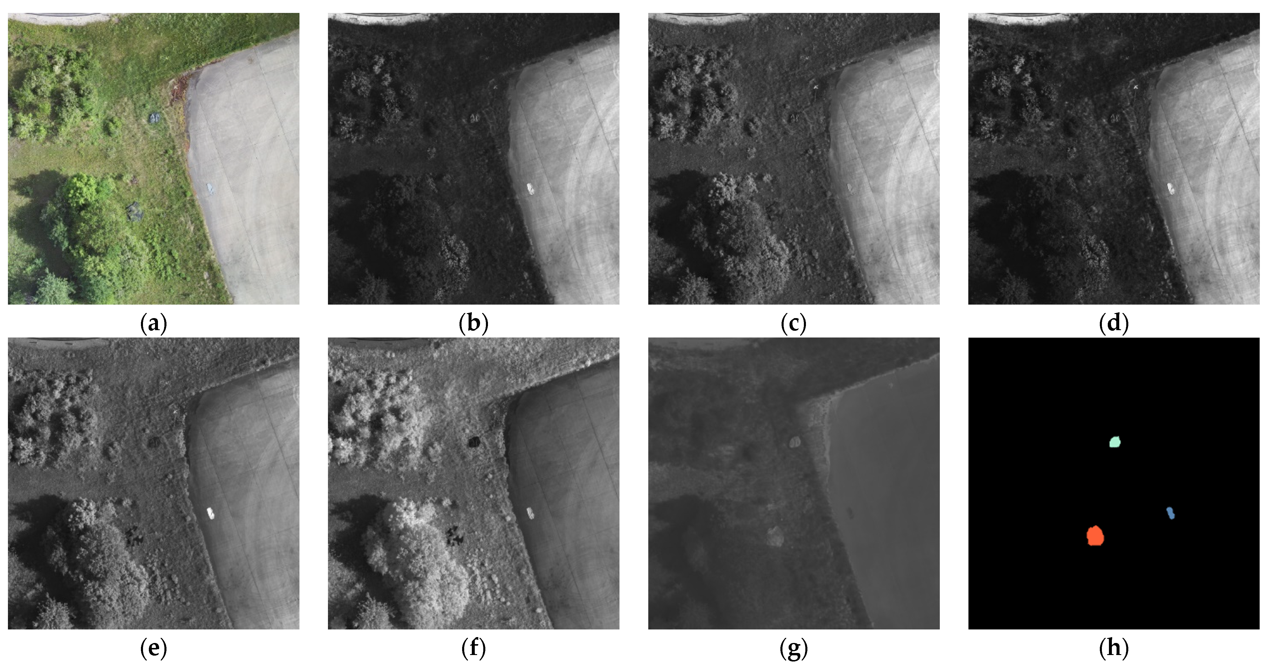
The multispectral dataset for camouflage detection (MUCAD) consists of 23 samples, each featuring 7 images with a resolution of 512 × 512 pixels and a corresponding ground truth mask containing target annotations. All images have a color depth of 8 bits and a ground sample distance (GSD) of 10 cm/px. Each kind of target is labeled with a different but consistent color across all samples. An example of a single sample is shown in
Figure 1. (a) shows the visual band (which is technically not a single band but is treated as such in this paper), (b–g) show the blue to LWIR bands, respectively, and are ordered by ascending wavelength and (h) shows the ground truth mask with annotations for a grey tarpaulin (dark blue), a green tarpaulin (light blue) and a 2D camouflage net (red).
The samples of the dataset were not natively captured but cut out of a set of geographically referenced and aligned orthophotos (one for each band). In addition, the samples were pixel aligned based on the ECC criterion [
33] using the implementation provided by OpenCV [
34] and rescaled to fit a resolution of 512 × 512 pixels and a GSD of 10 cm/px.
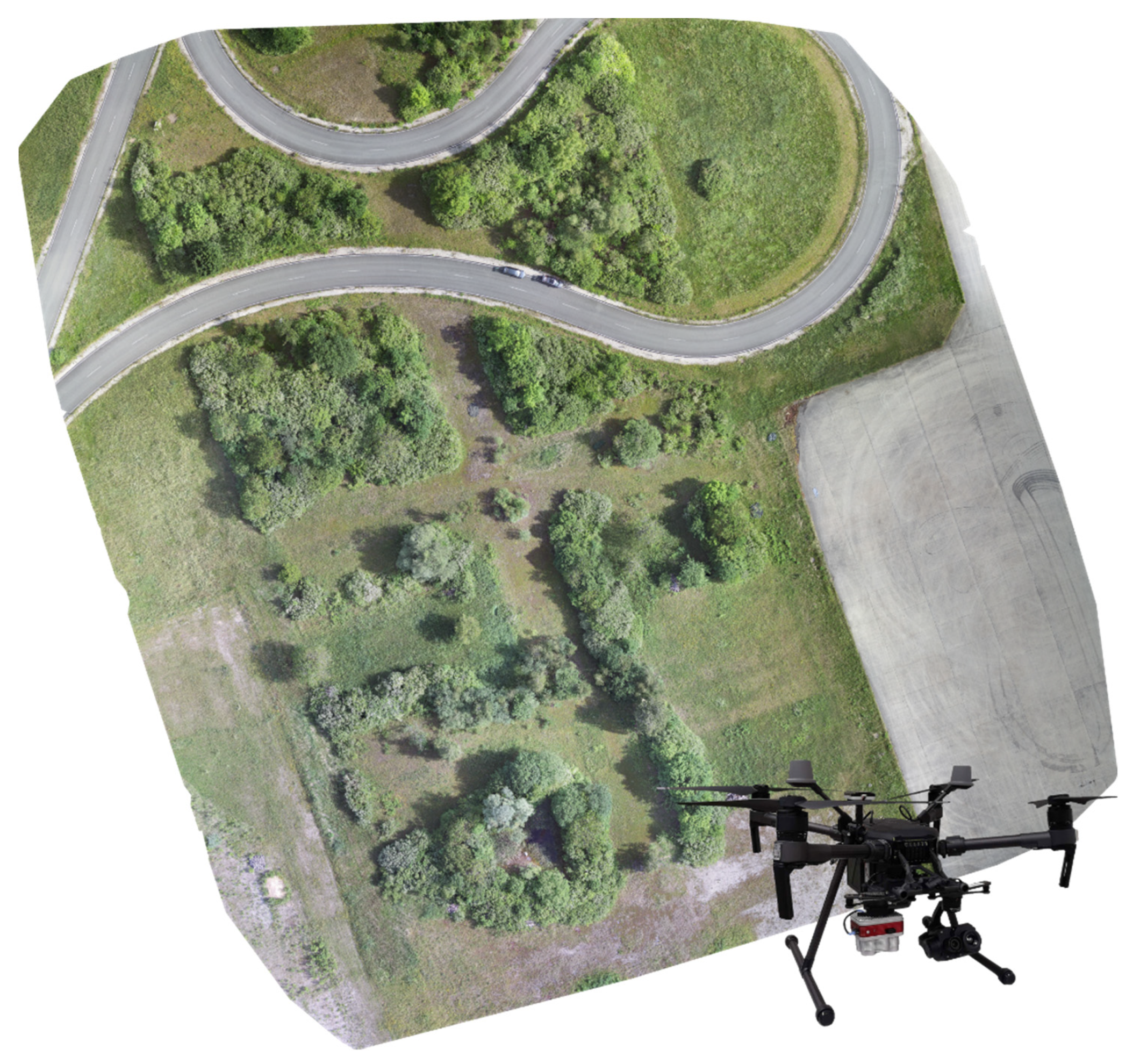
The orthophotos were generated using the aerial image mapping software OpenDroneMap [
35], where the raw sensor data were captured in 50 m height with 70% side and front overlap using a MicaSense Altum and a DJI Zenmuse XT2 mounted on a DJI Matrice 210 RTK V2. The complete setup, as well as a the generated visual orthophoto, are depicted in
Figure 2. Visual and LWIR images were provided by the Zenmuse XT2 and blue to NIR images were provided by the MicaSense Altum.
Table 1 shows further details about the captured spectral information of each band. Since both cameras capture images with 16-bit color depth except for the visual band, the intensities of all images were resampled from 16-bit to 8-bit color depth. Moreover, LWIR images were rescaled between their min and max values across all LWIR images before they were resampled down to 8-bit color depth. In contrast to common practices, the spectral bands provided by the MicaSense Altum were not converted to reflectance maps but kept in their raw form as reflectance values only matter for actual vegetational measurements which were not intended to be conducted.
The procedure for the dataset creation was chosen as it simplifies synchronization of both camera systems and allows the generation of images with arbitrary resolutions and ground sample distances only limited by the raw footage’s ground sample distance. The downside of this method is the inability to capture dynamic scenes.
Although this paper is about near real-time camouflage detection, the sensor–drone system in
Figure 2 itself does not allow near real-time image processing, as both camera systems only provide simple storage interfaces (USB stick and SD card), meaning that image processing must be performed offline. An on-board system capable of online image processing would have to be composed of sensor systems that provide a proper high-speed interface. Furthermore, setting up such a system would have required a different hardware platform and additional on-board processing capabilities. However, in creating the dataset, which theoretically could have been produced by a system with online capabilities, main concerns were fast and reliable raw data generation without excessive preliminary work, hence the hardware configuration described above. In addition, this paper only considers the near real-time capabilities (processing time less than one second) of the detection algorithms and not those of an entire system.
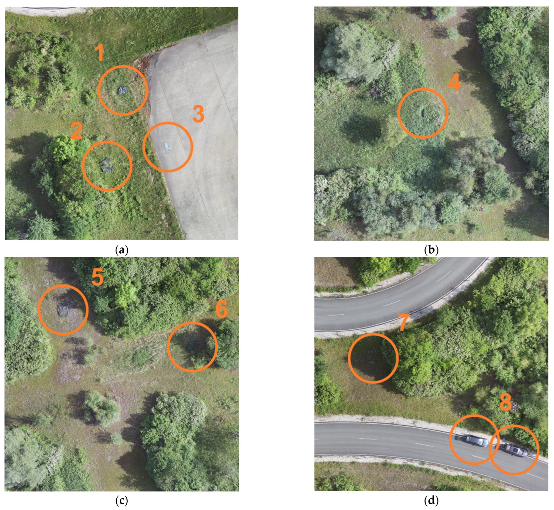
In total, MUCAD contains 8 different kinds of targets, whose placement is shown in
Figure 3. Each target was placed in a visually similar appearing environment. The first three target classes are depicted in
Figure 3a: (1) a green tarpaulin that was shaped to appear like a bush instead of a simple green rectangular, (2) a 2D camouflage net that was placed near the woods to appear like an extension of it and (3) a gray tarpaulin that was placed in a concrete area and additionally shaped to avoid sharp rectangular appearing transitions between the target and its environment. The fourth target is shown in
Figure 3b: (4) an artificial grass mat that was placed in very similar appearing high grass.
Figure 3c contains the fifth and sixth target classes: (5) a 3D camouflage net that was placed and shaped to appear like a tree crown or a bush and (6) an artificial hedge that was placed in a shadowed area and thrown over a bush to adapt its shape.
The last two target classes are shown in
Figure 3d: (7) two lying persons in a tree’s shadow wearing a battle dress uniform and a German field dress, respectively, and (8) two gray cars which were initially not considered targets but became targets as their color is close to that of the road but their heat signature is completely different.
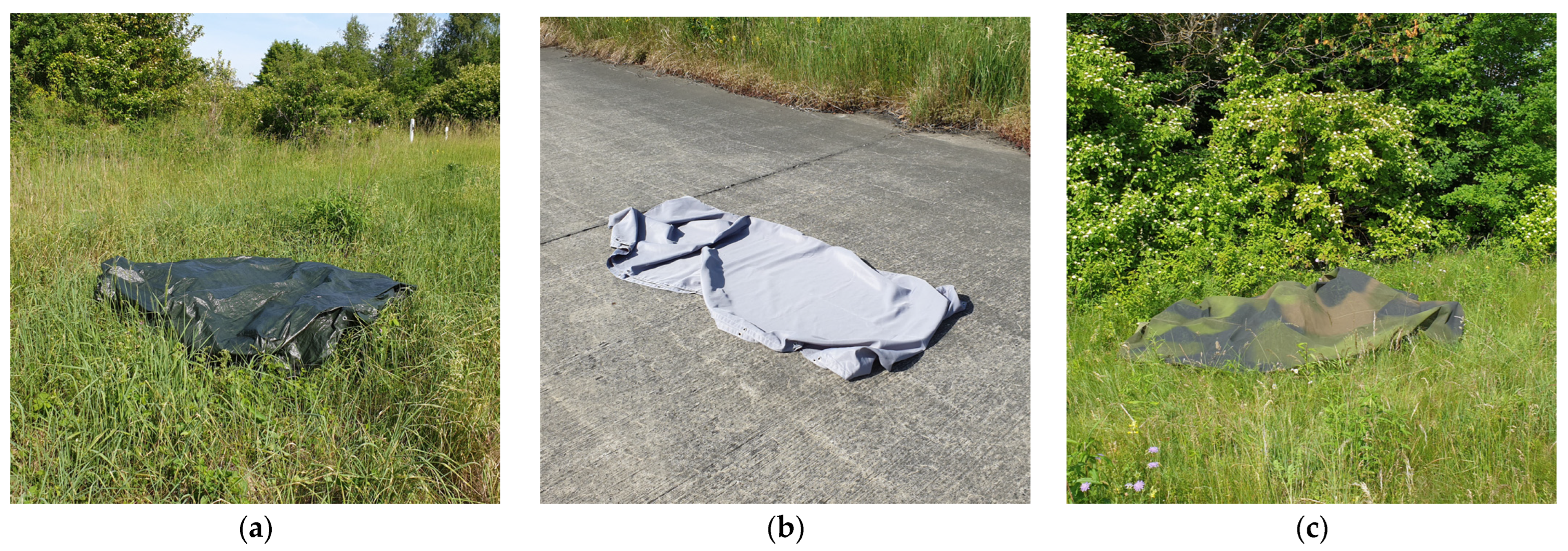
Figure 4 exemplarily shows the green tarpaulin, the grey tarpaulin, and the 2D camouflage net from the ground perspective just before they were captured by the multispectral camera system.
The targets were acquired from multiple different sources. The green tarpaulin, the gray tarpaulin, the artificial grass mat, and the artificial hedge were bought at a local hardware store to cover the use case of utilizing relatively simple means and easily acquirable materials to conceal objects in a suitable environment without having to shop online. To cover a classic military use case, additional camouflage equipment was bought online. According to the store pages, the 2D camouflage net and the 3D camouflage net were supposedly original equipment of the Bundeswehr (German Armed Forces) and the Armed Forces of the Crown (British Armed Forces), respectively. The German field dress and the battle dress uniform were also authentic original military equipment, according to the store pages.
In the dataset, every target is almost evenly distributed across all samples to keep a potential target class distribution bias as small as possible. Furthermore, to obtain more meaningful detection results, the samples were cropped from the orthophotos in such a way that each target is located in different parts of the captured area and that the same target has different backgrounds considering the whole area captured by the sample. For this reason, there are more samples than targets in the dataset.
The entire dataset was captured at the end of May 2021 at the test site of the Universität der Bundeswehr München and is publicly available (See the Data Availability Statement at the end of the article).
2.2. Camouflage Detectors
For the detection of camouflage in multispectral imagery, four well-known hyperspectral anomaly detection methods were adopted: the classic Reed–Xiaoli detector (RX) and local RX detector (LRX) [
21], the collaborative representation-based detector (CRD) [
22] and the attribute and edge-preserving filter detector (AED) [
23]. In addition to those four existing methods, this work introduces a new target detection method: local point density (LDP), which was inspired by dual window density (DWD) [
31].
While there are a lot of powerful options available, the methods were primarily selected by their prominence, expected implementation effort, and expected computational requirements, although covering a great variety of distinct approaches was also a major concern. For this reason, all methods are based on entirely different target and background modeling techniques. The methods and their implementations are briefly discussed in the following sections. For a deeper understanding of the algorithms’ theoretical foundations, versed readers may look up the provided references to the original publications.
2.2.1. RX and LRX
The RX detector [
21] is based on the assumption that spectral target and background signatures in an image can be modeled by a single gaussian distribution, respectively. Leading to the Mahalanobis distance for calculating an anomaly score for a single pixel:
where
is the resulting Mahalanobis distance for the pixel of interest,
is the corresponding pixel value vector,
is the mean vector consisting of the mean values for each band and
is the covariance matrix for the image’s bands. The higher the Mahalanobis distance for a single pixel the higher its anomality.
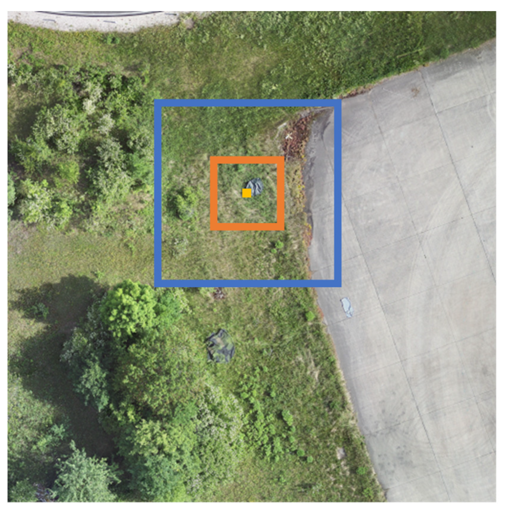
Instead of calculating the mean and covariance for the whole image, the LRX detector operates in a small local neighborhood for each pixel, defined by an inclusion and exclusion window size (
and
). Considering that every image possesses an arbitrary GSD and resolution and therefore also covers an arbitrary area in real-world space, it can make sense to restrict the region where mean and covariance estimation is performed to improve detection performance, as the whole image might cover multiple but entirely different backgrounds and targets.
Figure 5 shows the process of local neighborhood selection for a single pixel under test (marked yellow). The outer blue window describes the inclusion area, and the orange window describes the exclusion area, meaning that the mean and covariance for calculating the anomaly score (Mahalanobis distance) of the yellow pixel are estimated with all values that are contained in the blue window but are outside of the orange window. Conclusively, the LRX detector is computational more expensive than the plain RX detector but might achieve higher detection rates because of its local nature.
Both algorithms were implemented in C++ using Eigen 3 [
36], parallelized using OpenMP [
37] and not modified in any way they work. Additionally, the algorithms were interfaced for the us in Python 3 using Cython [
38].
2.2.2. CRD
Collaborative representation-based detection [
22] operates like the LRX detector in a local neighborhood (see
Figure 5), but works entirely different in calculating a pixelwise anomaly score. In general, it is assumed that a non-anomalous pixel can be collaboratively represented by a weighted sum of its neighboring pixels. The neighboring pixels are the pixels in the local neighborhood defined by the exclusion and inclusion area of the pixel under test. Consequently, it is also assumed that an anomalous pixel cannot be collaboratively represented by its neighboring pixels. The problem can be described as an optimization problem for a pixel vector under test
and its dual window neighborhood
:
where
is a 2D Matrix of size
containing all pixel values in the dual window neighborhood of the pixel under test.
is the value of the pixel under test,
is the weight vector whose elements describe the individual contribution of each pixel in the neighborhood and
is a regularization parameter that controls the weight of the penalty of the weight vector’s squared second norm. Fortunately, the optimization problem has a closed form solution and must not be solved iteratively (
is the identity matrix):
After obtaining the weight vector
for a pixel under test, its anomaly score a can be calculated, which is its reconstruction error at the same time:
The authors of CRD introduced an additional distance-based regularization method and a sum to one constraint for the weight vector. Details can be found in the original publication [
22]. For the implementation in this work, both concepts were applied.
Although CRD is a rather slow method, it was initially thought that it can be greatly accelerated by parallelizing it with a graphics card. Unfortunately, the matrix inversion in Equation (3) turned out to be too complex for a single graphics card core, leading to an even slower solution than a parallelized C++ implementation using Eigen 3 [
36] and OpenMP [
37] that was used for the results in this paper (additionally interfaced with Cython [
38] for the use in Python 3).
2.2.3. AED
In attribute and edge-preserving filtering-based anomaly detection (AED) [
23], it is assumed that anomalous objects are generally small and characterized by a significantly different intensity in a lot of bands compared to their backgrounds. In order to transfer that assumption into an algorithm, the authors utilized morphological attribute filters [
39] to decompose the image under test into morphological attribute profiles (APs). In detail, for each band two versions (the APs) are generated. One where all bright connected components that have an area (number of pixels) lower than
have been removed and one where all dark connected components that have an area lower than
have been removed. These two versions are subtracted from each other to obtain a difference map that has very large values where very bright or very dark connected components have been removed. All difference maps undergo a special binary filtering step where only the pixels with large values are retained and all others are set to zero. The filtered difference maps are finally accumulated into a single anomaly map, which is processed by an edge-preserving filter. Consequently, the final anomaly map has high values where a lot of connected components have been removed that had much lower or higher intensities compared to their backgrounds, thus indicating anomalous objects. It should be noted that the original AED algorithm performs a dimensionality reduction step on the image before it is further processed. This step was not deployed in this work, since it deals with multispectral imagery, which is of low dimensionality by nature.
In addition to the originally proposed algorithm, a version with an extra filtering step right after the binary filtering step that removes every bright connected component with an area lower than or a compactness (area divided by the square of its perimeter length) lower than was implemented. This additional filtering step is supposed to eliminate false positive detections in each individual band before they are combined into a single anomaly map. The customized version of AED is called AED-F (F for the additional filtering).
To reduce implementation effort, the edge-preserving filtering step for the final anomaly map in both algorithms was achieved by a common bilateral filter [
40] instead of a domain transform recursive filter [
41] utilized in the original publication [
23].
AED and AED-F were implemented in Python 3 using sap [
42] and OpenCV [
34].
2.2.4. LPD
Inspired by DWD [
31], a density-based [
43] algorithm was developed that encompasses a comparatively less memory intensive and more equally weighted pixelwise density computation, called local point density (LPD). LPD operates like LRX and CRD in a local neighborhood that is defined by an inclusion and exclusion area, as it is shown in
Figure 5.
For a pixel under test, its density is calculated according to:
where
is the pixel value vector,
is the i-th element of
and
is the size of
(
).
is the pixel’s dual window neighborhood of size
.
is the cut-off distance, which in contrast to DWD is not determined by calculating a distance matrix containing all distances between all pixel values but by computing the average distance between all pixel values and the average pixel value:
Compared to calculating a distance matrix, this method is much less memory expensive, as it is purely iterative and no matrix must be stored at all, which can prove useful in large scale parallelized implementations and on memory limited platforms.
The density calculated per pixel is additionally more evenly weighted compared to DWD, as pixel density is calculated pixel-wise with respect to a local neighborhood which is not the case in DWD, where pixel density is calculated window-wise with respect to a local neighborhood, meaning that the local neighborhood is not centered around every pixel under test as it is in LPD.
In the final density map, anomalous and background pixels have a low and high density, respectively. The density map is converted into an anomaly map by negating it and adding the lowest value to all pixels afterwards to avoid negative values.
LPD was implemented using C++ and Eigen 3 [
36], parallelized using OpenMP [
37], and interfaced for use in Python 3 using Cython [
38].
2.3. Vegetation Indices
As stated in the introduction, the methods described in
Section 2.2 were applied to two different configurations of MUCAD. First, on raw MUCAD, and second, on MUCAD-VI, which is an extension of MUCAD with the vegetation indices BNDVI, GNDVI, and NDRE, as it is described in
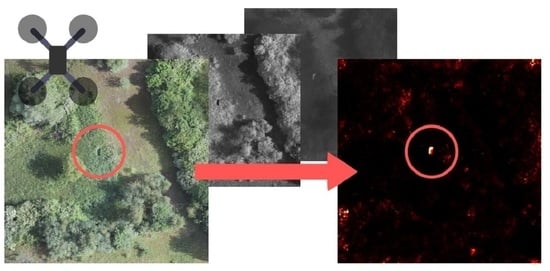
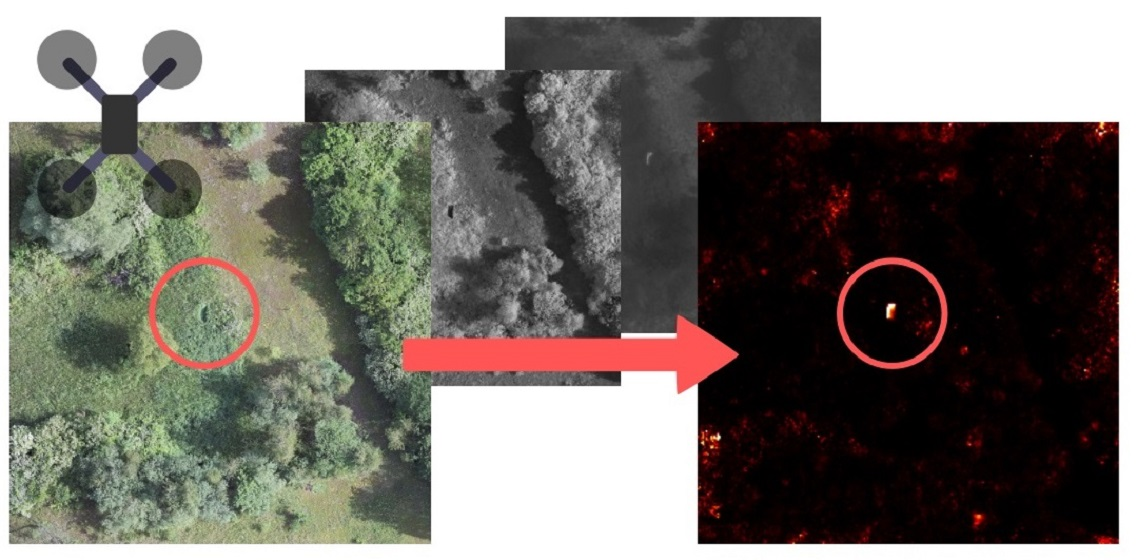
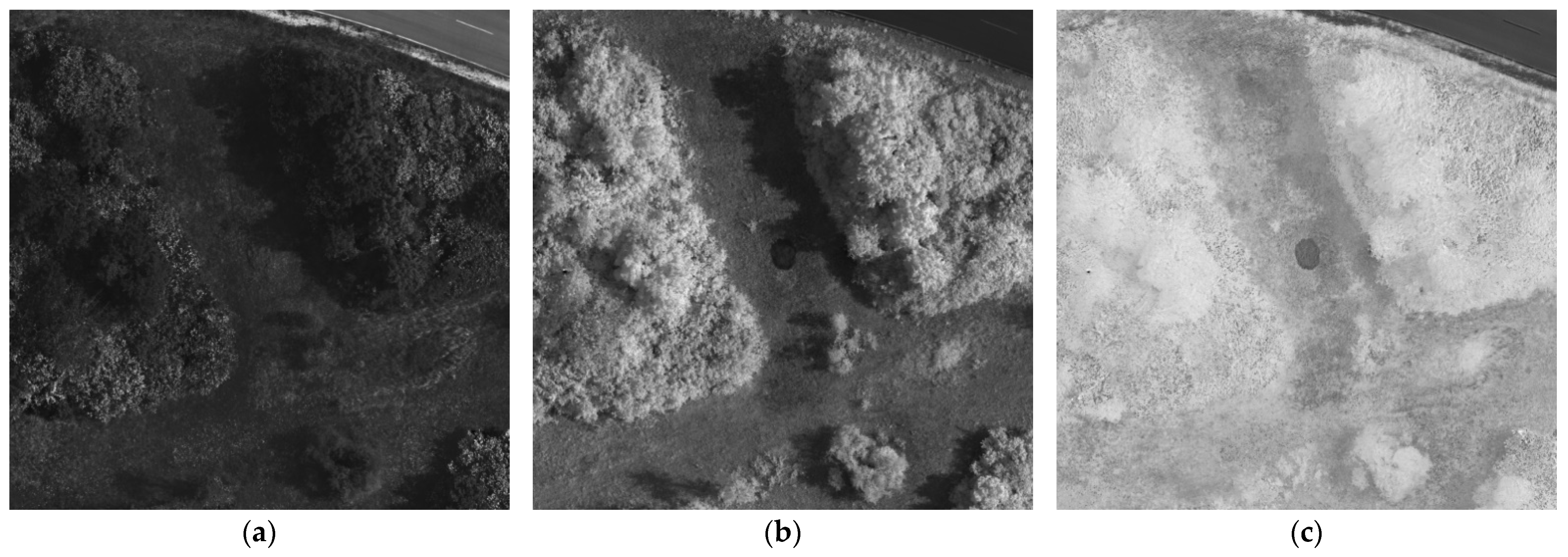
Table 2. The indices were chosen as they appeared to be increasing the visibility of some targets with respect to their environments (see
Figure 6), which could support successful target detections. All indices were computed online, meaning that they were not statically saved as files but calculated right before the detection algorithms were applied.
3. Results
For the evaluation of each target detector with MUCAD, an image resolution of 256 × 256 pixels was chosen to conserve computing capabilities, resulting in an effective ground sample distance of 20 cm/px for each sample. It is the lowest resolution that still allows for visually detecting the smallest targets of the dataset (persons in uniforms). Before the samples were processed by the algorithms, every band was z-normalized (mean of zero and standard deviation of one). Additionally, the visual band was weighted by one-third, since it was treated as a single band but technically consists of three individual bands. As a postprocessing step, all bright connected components that had an area smaller than nine pixels were removed in the final binarized anomaly map of each target detector, as it was assumed that anomalous objects occupy an area of at least a third square meter ().
To find a near to optimal configuration for each target detector, multiple parameters sets were applied (except for RX, which is parameterless). For LRX and LPD, and were set to: . Because of its expensive computational requirements, the window sizes of CRD were selected slightly differently: . As for the AED-based methods, was set to: . For AED-F, was also set to nine and (compactness threshold) was set to 0.15.
The target detectors were applied on two different dataset configurations: the raw version of MUCAD and an extended version with three additional bands: BNDVI, GNDVI, and NDRE. The evaluation of each method was performed based on its receiver operating characteristic (ROC) and the corresponding area under the curve (AUC). ROCs were calculated for each target class and each capture individually, which were then combined by threshold averaging [
44] afterward to obtain a single ROC for each target class over the whole dataset. ROCs with an AUC lower than 0.9 had such bad detection rates (true positive rate) and high false alarm rates (false positive rate), that they were considered to have not detected the target at all. Therefore, those weak results are not included in the following tables and graphs for better clarity of the remaining results.
All experiments were conducted on a machine running Ubuntu 20.04 LTS with an AMD Ryzen 9 3950X (16C/32T) and 128 GB Memory.
3.1. MUCAD
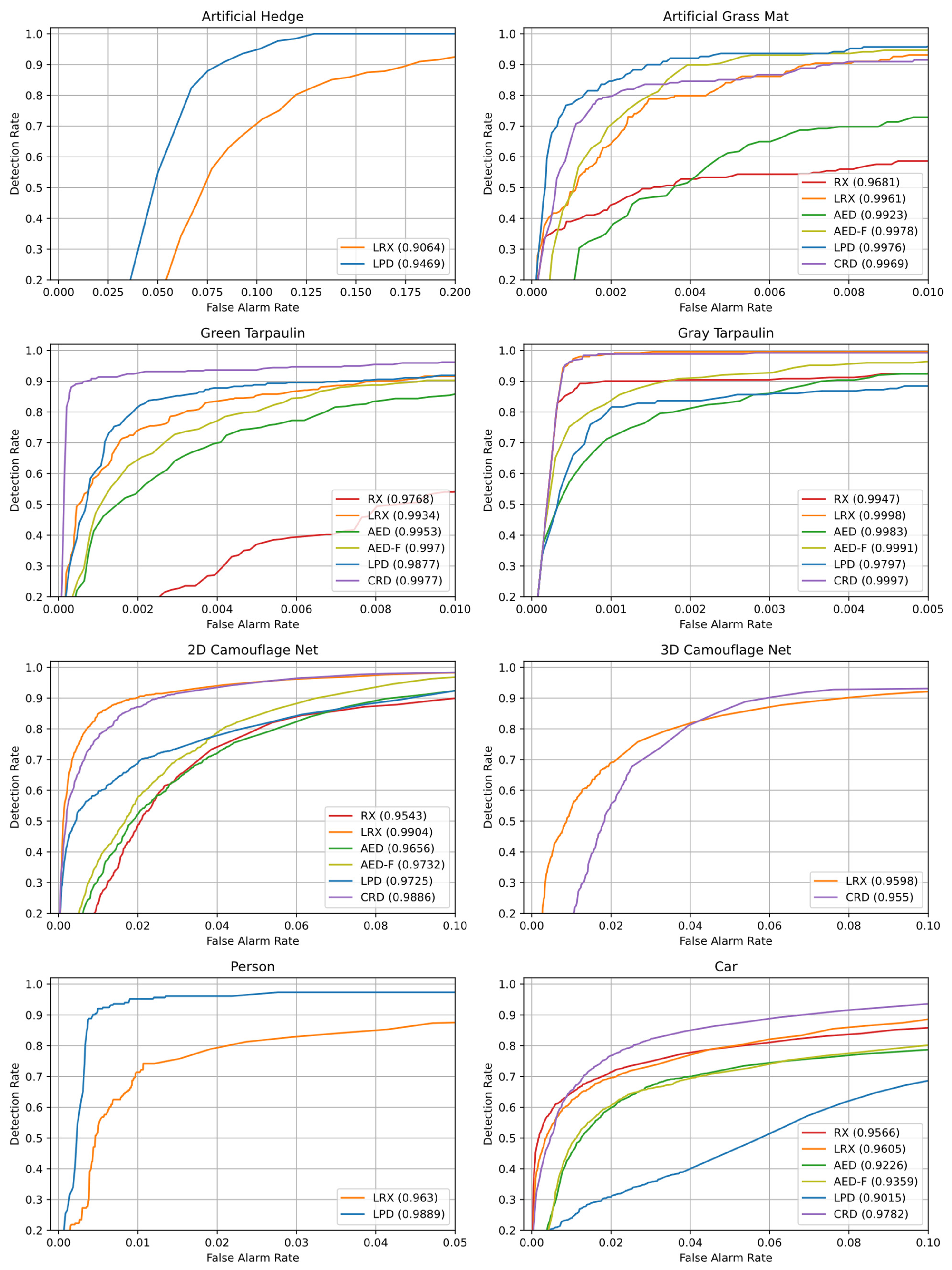
First, all target detectors were applied on the raw version of MUCAD. The resulting receiver operating characteristics are displayed in
Figure 7. Note that for each method only the parameter configuration that achieved the highest AUC over all parameter configurations of the method is shown. All other parameter configurations are not further considered in the following evaluation. Each tile shows the results for a specific target class and contains a color-coded ROC for every successful algorithm (note that each plot has individual limits for the abscissa). The legend of every tile shows AUCs for each ROC in parentheses.
As it can be seen, detection performances vary greatly across target detectors and classes. The artificial hedge could only be detected by LRX and LPD. Still, their AUCs are relatively low, and ROCs show that false alarm rates are already considerably high before detection rates even reach 50%, which signalizes high difficulty for the methods to detect the target. In contrast to that, the artificial grass mat, the green tarpaulin and the gray tarpaulin were detected by all algorithms with high detection rates at low false alarm rates. The 2D camouflage net, as well as the cars, were also detected by all methods but with significantly lower performance, although LRX and CRD stand clearly out in AUC and ROC. For the 3D camouflage net, only LRX and CRD could achieve considerable results. Yet, the detection performances are almost as bad as for the artificial hedge, making it the second target that could barely be detected. The persons were also detected only by two algorithms: LRX and LPD. Only this time, LPD achieved a comparatively strong performance with high detection rates at low false alarm rates.
Table 3 contains the AUCs, parameter configurations, and runtimes for the ROCs in
Figure 7. The upper third of the table shows the AUC values of each algorithm for every target class where the highest values are marked bold. As mentioned before, AUC values lower than 0.9 are not included and were replaced by a “-”. Top scores are almost evenly spread across LRX, LPD and CRD, showing that the detection task benefits from local target and background assumptions, while the plain RX detector stays noticeably behind the top performances in all target classes except for the gray tarpaulin. AED-based methods fail in as many target class detections as RX but achieve close to best performance for the artificial grass mat, the green tarpaulin and the gray tarpaulin. Moreover, AED-F achieves consistently higher AUCs compared to its unmodified counterpart AED, showing the effectiveness of the additional filtering. As already pointed out based on the ROCs, the artificial hedge, the 3D camouflage net and the persons cannot be detected by a lot of algorithms, though LPD achieves a strong detection performance for the person target class. Those bad detection performances are likely due to weak spectral differences of the artificial hedge (which even lies in the shadows) and the 3D camouflage net, and the small spatial size of the persons, making them particularly hard to differentiate from normal background clutter.
The middle third of the table describes the parameter configuration for each detector whose AUC is given in the first third. Depending on the algorithm, values stand either for the inclusion and exclusion window ( and ) or for the area of connected components to be removed (). RX is parameterless. For the local neighborhood-based algorithms, window sizes logically rise and fall with the targets’ sizes. As does the connected component area for the AED-based methods.
The runtimes of the algorithms are outlined in the lower third of the table. The RX detector does not have any parameters which results in a consistent runtime for each target class. LRX, LPD and CRD depend heavily on their parameters, which translates into increasing runtimes for larger window sizes. The runtimes of the AED-based methods are not influenced by their parameters and are therefore constant for each target class, although the additional filtering in AED-F almost doubles its time consumption. CRD has striking high runtimes due to its computational complexity, making it unsuitable for any near real-time application regardless of its strong detection performance. All other methods keep their time consumption below one second except LRX, which exceeds it when window sizes are comparatively large. Note that the runtimes only contain the raw method execution time and no time consumption caused by pre- or postprocessing.
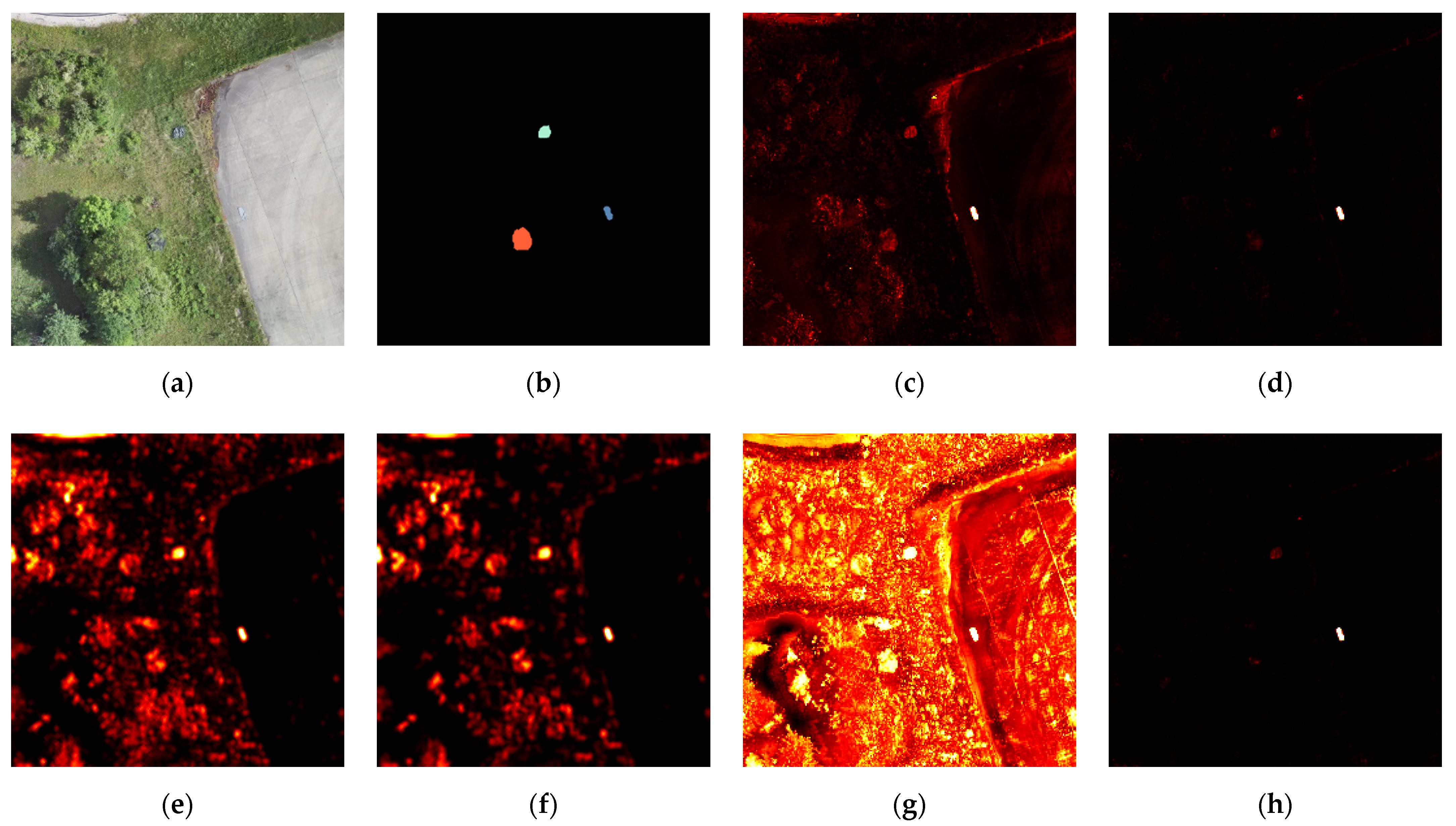
Figure 8 shows the detection maps of all methods for an exemplary capture of MUCAD containing the green tarpaulin, the grey tarpaulin, and the 2D camouflage net. The first two images show the visual band (a) and the associated ground truth (b) of the capture, followed by the detection maps (c–h) of RX, LRX, AED, AED-F, LPD, and CRD, respectively. The parameter configurations of each method correspond to the second column in
Table 3. As it can be qualitatively observed, AED-F (f) produced much fewer false positives in the detection map compared to AED (e). LRX (d) also generated much fewer false positive detections than RX (c), which is consistent with their corresponding ROCs in
Figure 7 and AUCs in
Table 3. LPD (g) produced a significantly different detection map with generally higher anomaly scores compared to all other methods, but with no apparent negative impact on its ROC or AUC. The detection map of CRD (h) appears to be very similar to the detection map of LRX (d), although there are generally considerable differences in detection performance, as indicated by their ROCs and AUCs.
3.2. MUCAD-VI
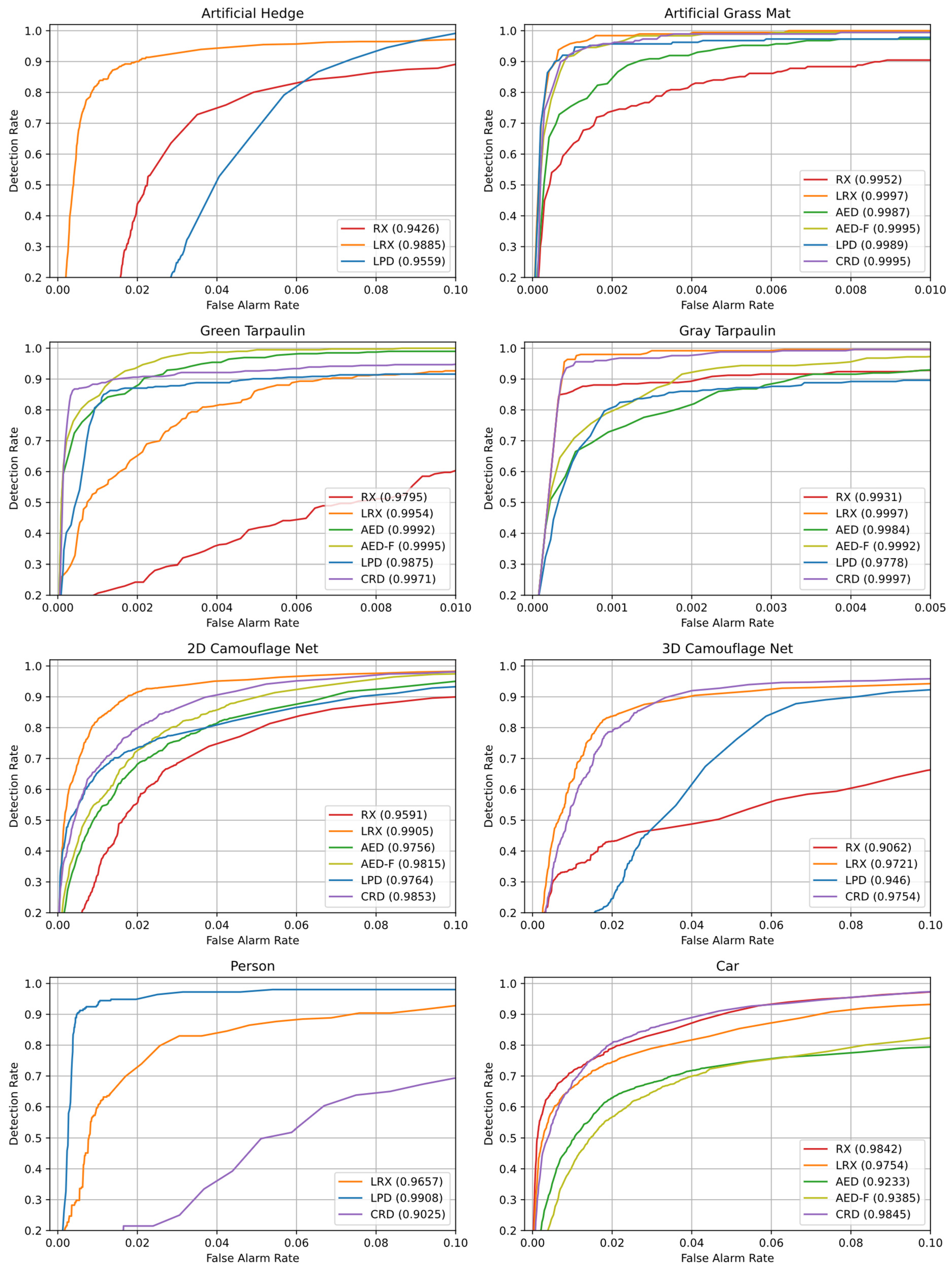
For the extended version of MUCAD (MUCAD-VI), receiver operating characteristics for every target class are shown in
Figure 9. The tiles and their contents follow the same pattern as in
Figure 7. For the artificial hedge, only a subset of algorithms (RX, LRX, and LPD) could achieve more than 0.9 AUC, but LRX obtained much higher detection rates at equal false alarm rates compared to RX and LPD. The artificial grass mat, the green tarpaulin, and the grey tarpaulin were detected by all algorithms, with LRX, CRD, AED, and AED-F being close to an ideal detector for certain targets. All methods could detect the 2D camouflage net, although LRX clearly outperformed all other detectors. For the 3D camouflage net, only LRX and CRD could achieve comparatively high detection rates at low false alarm rates. LPD and RX obtained indeed more than 0.9 AUC but performed significantly lower than their competitors. The persons were detected solely by LRX, LPD, and CRD, with LPD clearly dominating in high detection rates at low false alarm rates. For the detection of the cars, RX, LRX, and CRD obtained very similar results and outperformed all other methods, with LPD not even reaching 0.9 AUC.
Compared to the ROCs in
Figure 7 (raw MUCAD), detection rates at low false alarms generally improved across all methods and target classes. Most noticeable, the artificial hedge (which was barely detected by LRX applied on the raw version of MUCAD) could be detected with much higher detection rates at much lower false alarm rates. Additionally, targets that were detected only by two methods in MUCAD, were detected by three to four methods in MUCAD-VI. Although LPD previously managed to achieve more than 0.9 AUC for the cars, its detection performance fell below that threshold in its application on MUCAD-VI.
Table 4 contains AUCs, parameter configurations, and runtimes for the methods and ROCs in
Figure 9. In the first third of the table, the detection performances in AUC are displayed, with the highest value per target class marked in bold. LRX and CRD are clearly dominating in terms of the number of highest AUC per class. AED-F and LPD achieved a single top result, respectively, while RX and AED did not achieve any of the top results. Additionally, LRX is the only algorithm that detected all targets (more than 0.9 AUC for all targets). RX, LPD, and CRD could not detect the persons, the cars, and the artificial hedge, respectively. In addition, not having accomplished top results in each class, it is notable that AED-F achieved results relatively close to an ideal detector for the artificial grass mat, the green tarpaulin, and the gray tarpaulin.
As it has already been pointed out in the evaluation of the ROCs in
Figure 9, compared to the results obtained with raw MUCAD, detection performances for MUCAD-VI consistently increased or were at least equally high. This is most noticeable for the artificial hedge and the 3D camouflage net, which were most difficult to detect by all algorithms (lowest AUC values). Furthermore, targets that were detected only by a small subset of methods before, were detected by one to two methods more.
The parameter configurations in the middle third of table, indicating either the inclusion and exclusion window sizes or the area of connected components to be removed, do not show any significant changes compared to the parameter configurations of the methods when applied on raw MUCAD.
The opposite situation prevails for the runtimes in the lower third of the table. While RX and CRD seem to be almost unaffected by the increased number of bands in MUCAD-VI, all other methods show considerable higher runtimes. LRX needs roughly twice as much time and the AED-based methods apparently scale linearly with the number of bands to process. LPD is less sensitive to the number of bands, resulting only in a marginally higher time consumption for the same parameter configurations.
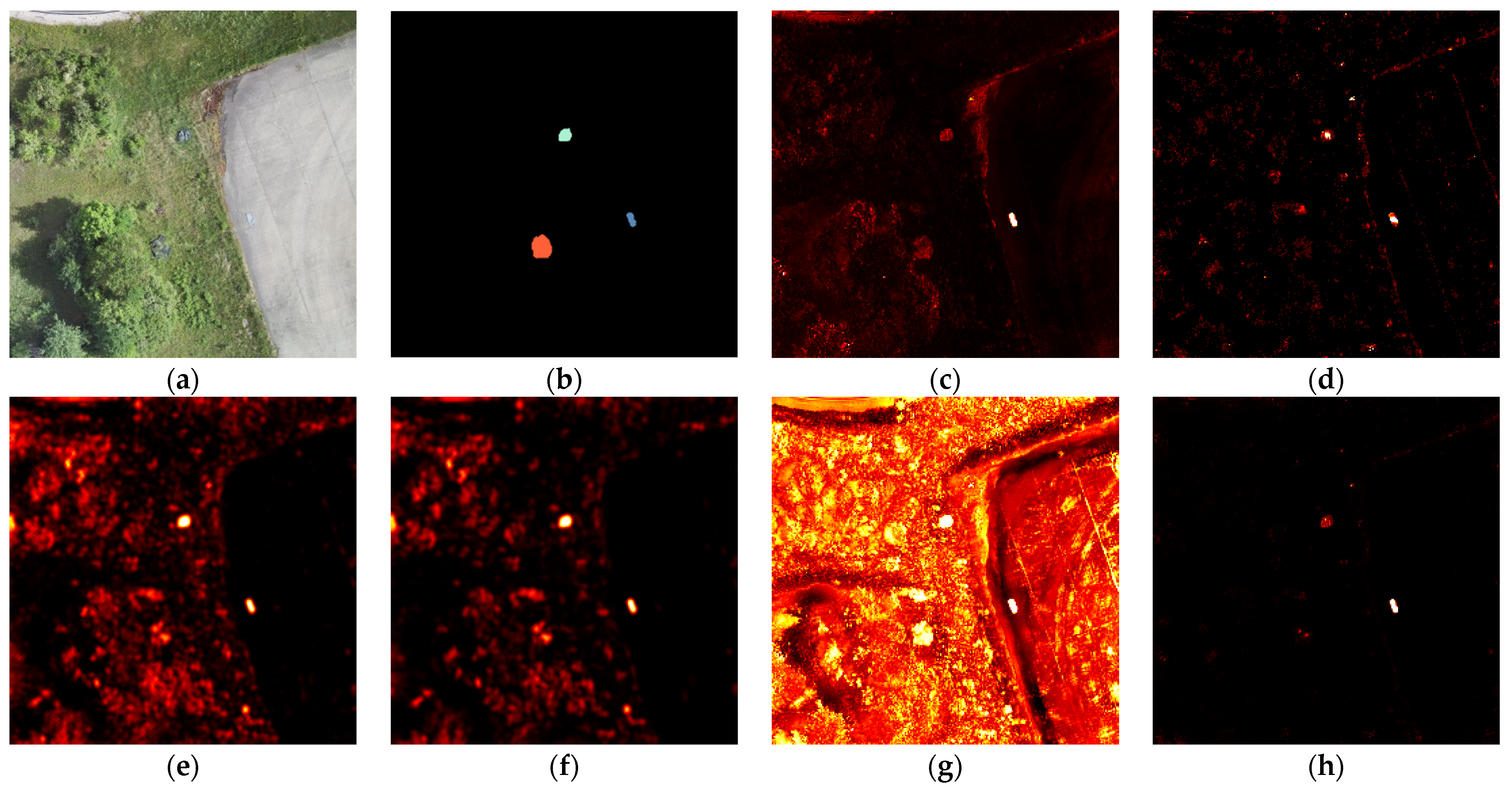
Figure 10 shows the detection maps of all methods for an exemplary capture of MUCAD-VI containing the green tarpaulin, the grey tarpaulin and the 2D camouflage net. The images (a–h) follow the same structure as the images in
Figure 8. The parameter configurations of each method correspond to the second column in
Table 4. Compared to the detection maps in
Figure 8, the anomaly scores in the target areas are considerably higher, particularly in the detection maps of AED (e) and AED-F (f), which qualitatively confirms the generally higher detection performance of all methods observed in the ROCs of
Figure 9 and the AUCs of
Table 4. AED-F (f) again generated much fewer false positives than AED (e), as did LRX (d) compared to RX (c). In contrast to
Figure 8, CRD (h) produced a detection map with significantly fewer false positives compared to LRX (d).
4. Discussions
The results showed that all adopted anomaly detection methods were principally capable of detecting multiple targets in MUCAD and MUCAD-VI, clearly indicating the applicability of hyperspectral anomaly detection methods for camouflage detection in multispectral imagery. However, none of the detectors could achieve strong and stable results over all targets, although LRX was the only method that obtained more than 0.9 AUC for all targets. Yet, the detection performances of all methods including LRX heavily fluctuated across all targets. For instance, LPD outperformed all other methods for the relatively small person targets but achieved considerably worse results than LRX for all other targets, which indeed works entirely different but operates in a local neighborhood very similar to LPD. In addition, the AED-based methods achieved top detection performances for the artificial grass mat, the green tarpaulin, and the gray tarpaulin but far worse results for all other targets. The high detection rates for those specific targets might be induced by the very homogenous surfaces and strong spectral distinctiveness compared to the other targets. These observations indicate that each algorithm heavily depends on the target’s properties for successful detections. As already indicated in the introduction, it is the nature of camouflage that its spatial and spectral properties are usually unknown in real-world reconnaissance scenarios, which makes it very difficult to account for these strong dependencies. Fusing anomaly maps of different (or differently configured) target detectors that were empirically evaluated to work for targets featuring specific properties with very low false alarm rates could be an applicable approach to mitigate that issue to some extent.
It must also be noted that all detectors generally depend on strong spectral differences between targets and their surroundings, which is a logical requirement for the detectors to work but must be considered for the evaluation of each detector. For example, the artificial hedge lacks strong spectral distinctiveness in its environment as it is occluded by shadows, but all bands except LWIR of MUCAD and MUCAD-VI depend on the target’s reflectance properties which are naturally less prominent in low light environments. Therefore, the algorithms had to detect targets with very little anomalous spectral characteristics, which is of course more difficult than the detection of targets with strong anomalous properties. The artificial grass mat, the green tarpaulin, and the grey tarpaulin possess very distinctive and unique spectral signatures, which resulted in significantly high detection rates at low false alarm rates for all algorithms compared to all other targets. In this context, it becomes apparent that the successful detection of certain targets in certain environments depends not only on the detection algorithms but on the underlying multispectral sensor setup or dataset, as well. Since the environments and targets captured in MUCAD are limited, the results account only for a very limited scope of possibilities. For different targets and different environments, the multispectral sensor setup might be not suitable to provide distinctive spectral signatures for each target, which in turn might then not be detected by any algorithm.
Although the selection of vegetation indices added to MUCAD in MUCAD-VI may seem arbitrary, the results indicate that a combination of the existing bands can have a positive effect on the performance of the target detectors. Since the sensor setup or the dataset is usually fixed in terms of bands and spectral raw information, an extension of more deliberately chosen combinations of bands might even further improve the detection performances compared to a selection of already predefined vegetation indices.
In terms of computational complexity and runtimes, all target detectors except CRD were able to work at near real-time conditions under most circumstances. Only a few parameter configurations led to runtimes slower than one second, although the number of bands to process had some influence, as well. In real-world applications with near real-time requirements, parameter configurations and the number of bands under consideration must be properly selected to avoid excessive runtimes of sensitive algorithms. However, it must also be noted that all runtimes were measured on a currently very powerful CPU, which might not be available in real-world scenarios. Despite its strong detection performance, the implementation of CRD in this work always requires much more time than a single second and does therefore not fulfill near real-time requirements, making it currently unsuitable for any real-world application.
Future research will focus on further improving the detection results by collecting more multispectral data at different seasons and by investigating how multispectral raw bands can be effectively enhanced, (i.e., by combining them) and selected in order to maximize the visibility of camouflage in different environments.
5. Conclusions
From the evaluation of the detection performances, it can be concluded that the hyperspectral anomaly detection methods investigated in this paper can principally be used for camouflage detection in multispectral imagery. However, since all methods already showed strong variations in detection performance for the limited number of different targets and environments in MUCAD, it must be assumed that even the best detection algorithm could miss some targets in real-world applications. As failing to detect a camouflaged hostile unit could prove fatal in a real-world reconnaissance scenario, additional research must be conducted to further improve detection results.
In addition to the individual detector performances, the limited spectral information provided by any multispectral sensor setup or dataset must also be taken into account. Some spectral bands may not contain enough information for certain targets and environments in order to lead to successful target detections. As shown in the results, enhancing the data with carefully selected derived bands, such as vegetation indices, can successfully mitigate that issue and result in higher detection rates of the algorithms.
Since multispectral imagery is not as complex as its hyperspectral counterpart, nearly all detectors except CRD performed at near real-time requirements. However, some algorithms quickly slowed down as the number of bands to process increased or their parameters changed, which must be considered in a tactical reconnaissance scenario where time is of the essence. The number of bands to process should therefore be kept as low as possible and the parameter configuration carefully selected to minimize computation time.


